TítuloStatistical Applications to Thermal Analysis

Ricardo Cao and Salvador Naya

Departament of Mathematics. Universidade da Coruña [email protected]

1. Application of nonparametric regression methods 1.1. Introduction

An important topic in thermal analysis is the statistical analysis. There are several works in the thermal analysis literature that use regression models to account for the relationship between the variables of interest in this field. Many of them are based on the Arrhenius equation modified by Sestak and Berggren [27] and were discussed by Vyazovkin [29] and compared by many authors [3].

The response variable is often heat flow or sample mass along the experiment, while typical explanatory variables are temperature or time. Some important properties of the materials can be directly measured or easily calculated from the response variables. They include characteristic temperatures of different processes, i. e. melting and glass transition temperatures, thermal stability, specific heat at different temperatures, enthalpy associated to chemical reactions and physical changes. In addition, kinetic analysis of the processes can be performed from the thermal analysis data. The study of these data gives useful insight for materials characterization.

It is relevant to point out that the estimation of the first two derivatives is also an important issue. In the case of weight loss processes, the TGA first derivative (DTG) can be compared to the DSC trace. The DTG trace is sharper and more accurate to detect the onset and end points of the processes. It is especially interesting when studying overlapped processes. This higher quality of DTG compared to DSC comes from two differences between the both techniques:

1. The TGA response is almost instantaneous and immediately reflects the weight changes, while the DSC signal is affected by a thermal lag (the heat from the sample takes some time to travel through the crucible to the detector).

2. The heat diffusion in the crucible smoothes the signal before reaching the detector.

TGA and DSC, therefore, give direct mass and calorimetric measurements for whose a good estimation accuracy is desired.

The main aim of this work is to accurately estimate the functional relationship between an explanatory variable X, typically time or temperature, and a response variable Y, often weight (for TGA curves) or heat flow (for DSC curves). The following nonparametric regression model is assumed to hold:

. , , 2 , 1 , )

(X i n

m

Yi = i +εi = with E(εi)=0. (1)

where m is the regression function of Y given X and εi is a term accounting for the

The methods used in practice to smooth DSC or TGA curves by means of nonparametric weights do not incorporate any automatic optimal smoothing parameter selection. In some cases they are even based in moving average procedures, going back to the early work by Savitzky and Golay [25]. For this reason the bad fitting is very evident in many cases, specially in the first and second derivative estimation.

0.0 10.0 20.0 30.0 40.0 50.0 60.0

-2.0

-1.5 -1.0 -0.5 0.0

0.5

2.0

3.0 4.0 5.0 6.0 7.0

8.0

t ime [min]

d(

W

e

ig

ht

)/

d(

ti

m

e

) (

)

[]

We

ig

h

t (

)

[m

g

]

calcium oxalate_1

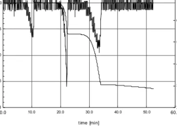
Figure 1. TGA curve for the calcium oxalate sample (dashed line) and first derivative (solid line) using the RSI Orchestrator

Figure 1 shows a fit of a TGA curve of calcium oxalato and its first derivative using one of the standard computer packages in this field, the Orchestrator® by Rheometric Scientific Incorporation®. The smoothing software incorporated to this package enables selection of the amount of smoothing "by hand" but not any automatic estimated optimal smoothing parameter that takes into account the non negligible error dependence. The aim of this paper is precisely to provide an automatic selection of the amount of smoothing to be used in these contexts.

1.2. Technical background

Nonparametric regression methods will be used to estimate the function m

without specifying any a priori parametric model. The key idea is to assume that m is a smooth function and approximate m(x) by averaging the Y-observations in a neighbourhood of x:

¦

=

= n

i

i

ni xY

W n x m

1 ) ( 1 )

( , with

¦

=

=

n

i ni x W

1

. 1 )

( (2)

where )Wni(x is the weight that the i-th observation gives to the point x. Typically these

mention the Nadaraya-Watson estimator (see [18]), Priestley-Chao estimator (see [21]), Gasser-Müller estimator (see [16]) and the local polynomial estimator (see [9]).

Since our aim is to estimate the regression function as well as its first two derivatives it is very natural to use local polynomial estimators, which additionally have good properties for estimating at the boundary.

1.3. Local polynomial estimator

The local polynomial estimator was introduced by Stone [28] and Cleveland [5] but it has not been extensively used until the ninenties, after publication of the papers by Ruppert and Wand [23] and Fan and Gijbels [9].

The idea behind the local polynomial regression estimator is to use weighted least squares to perform a local fit to a polynomial of degree specified in advance. More precisely the regression function (j=0) and its derivatives (j=1,2,…,p) at a given point x are estimated by

) ( ! ) (

ˆ( ) x j x

m j ₌ β_{j j= 0,1,2,…,p, (3)}

where

(

)

(

)

β

β Y X W Y X

t

p = − −

= (4)

¸ ¸ ¸

¹ ·

¨ ¨ ¨

© § = ¸ ¸ ¸

¹ ·

¨ ¨ ¨

© §

− −

− −

=

n p

n n

p

Y Y Y x X x

X

x X x

X

X

1 1

1

, ) ( ) ( 1

) ( ) ( 1

andW =diag

{

(

)

}

(

)

=

β (5) 1.3.1. Practical choice of the kernel and the order of the local polynomial

In order to use the local polynomial estimator we need to choose the kernel function,K, the degree of the polynomial, p, and the bandwidth, h. The choice of K and

p is of secondary importance with respect to the smoothing parameter h. Fan and Gijbels [10] recommend using the Epanechnikov kernel, since it minimizes the asymptotic mean squared error for an optimal bandwidth. They also suggest to choose p

as any integer larger than the order of derivative of interest, j, such that p-j is odd. For instance we could take p=1 for estimating the regression function itself, while p=3 could be used for estimating the second derivative of the regression function. In general, based on the bias decreasing and variance increasing with p, an advisable practical choice is to setp-j=1,3.

Gasser [26], can be solved performing a local increasing of the smoothing parameter whenever it occurs.

For dependent data, as those we are dealing with, the classical local polynomial regression estimator can still be used, although its asymptotic mean squared error depends now on the sum of covariances of the error process. An alternative approach has been proposed by Francisco and Vilar-Fernández [13], by using generalized least squares ideas to account for the dependence structure.

1.3.2. Bandwidth selection criteria

Typical bandwidth selection procedures are based on minimizing the empirical version of some criterion that accounts for the error between the nonparametric Ȟ-th derivative regression estimation and its underlying counterpart. For instance, using the mean squared error at a given point x:

(

)

we obtain local optimal bandwidths. Global criteria, as the MISE, can be obtained by considering global distances between the estimator and the true curve. Most of the times these measures can be written as integrated versions of the some local criterion (Eq. 6). For instance the mean integrated squared error can be written as:

(

)

)

(h =E

_³

MISE_{x h} (7) for some weight function w. This measure can be easily decomposed as a sum of the integrated variance and the integrated squared bias.

Under independence in the error structure and assuming that Ȟ+p is odd, Fan and Gijbels [10] give asymptotic expressions for the bias and the variance of the local polynomial estimator:

(

)

(

)

{

}

In the dependent error case similar formulas can be obtained based on parallel expressions to bias and varianza (Eq. 8). For the asymptotic mean integrated squared error (see Francisco and Vilar-Fernández [13] for details) the following expression gives some approximation of a reasonable criterion to select h. Therefore, an asymptotically optimal bandwidth (in the sense of AMSE) to estimate the ȣ-th derivative of the regression function is:

(

)

(

)

1.3.3. Two-stage plug-in bandwidth selector

Some of the most popular procedures for bandwidth selection in nonparametric curve estimation are the plug-in methods. These methods estimate the minimizer of either the AMSE or AMISE. For the local polynomial estimator under dependence, the plug-in local and global bandwidth selectors are some estimators of expressions (Eq. 10 and 11). Therefore some estimators of c(ε), the sum of autocovariances, and the (p +1)-th derivative of +1)-the regression function are needed.

Estimating the autocovariances sum

Although c(ε)can be estimated through the spectral density of the εi our

process of order 1 (AR(1)) with first order autocorrelation ȡ. Then c(ε)can be written in terms of the error variance and the autocorrelation coefficient:

¦

¦

(

)

= −

ε and an estimator of the first lag autocorrelation coefficient:

(

)(

)

Pilot bandwidths choice

The plug-in method requires to estimate the unknown quantities in (Eq. 10 and 11) and by some values hPI,L and hPI,G. For a fixed integer, Ȟ, the method is used to

estimate mυ using local polynomials of degree p. Estimation of c(ε), already considered in the previous subsection, requires the choice of a preliminary bandwidth

1

h, needed to compute the residuals.

Plug-in bandwidth selectors also need to estimate the (p+1)-th derivative of the regression function, m. This may be done, once more, by means of local polynomial fitting for estimating the Ȟ derivative (Ȟ=p+1) using local polynomials of degree p+2. This requires the choice of a preliminary pilot bandwidth, (1)

2

h . To determine some automatic method for selecting (1)

2

h we face similar problems when looking at the expression for the optimal (local or global) smoothing parameter in this context. More specifically, there are two unknown terms to be estimated: c(ε) already considered above, and the (p+1)-th derivative of m. The idea behind the two-stage plug-in method is to propose some prepilot bandwidth, h2(0), by looking at the expression for the asymptotically optimal bandwidth for this new problem:

equispaced, we made the choice δ =(x_n−x₁)/(n−1). The value of C₂ has been adjusted by some heuristic approach to be detailed later.

Parallel problems appear when selecting h₁. In practice we used a local linear estimator and a single-stage plug-in procedure leading to:

5 1 1 1

−

=C n

h δ (15) for some constant C1 that has been obtained by heuristic arguments.

In order to obtain some practical value for the constants C₁ and C₂we use a calibration sample of a DSC curve. This sample of n=950 equally spaced data corresponds to calcium oxalate monohydrate. Using the initial bandwidth h₁=6 to compute the residuals for estimating the autocovariances sum, we have selected several possible values for the prepilot bandwidth (0)

2

h for which the final bandwidths of the two-stage plug-in procedure have been computed. The results are collected in Table 1. This table shows how the sensitivity of h_PI to the choice of the prepilot bandwidth,

) 0 ( 2

h , is very low. When estimating the regression function, a factor of 10 in the prepilot bandwidth gives a factor of 4 in the pilot bandwidth and finally a factor of 1.5 in the plug-in bandwidth.

For estimating the first and second derivatives, the plug-in bandwidth selector is rather stable with respect to the choice of the prepilot bandwidth, although not so much as for estimating m. Direct inspection of the results obtained (not reported here) show that h₁=6 is a reasonable choice. On the other hand, the values (0)

2

h =30, for m, (0) 2

h =28,

for mƍ and h₂(0)=30, for mƍƍ seem to be reasonable choices for the prepilot bandwidth )

0 ( 2

h

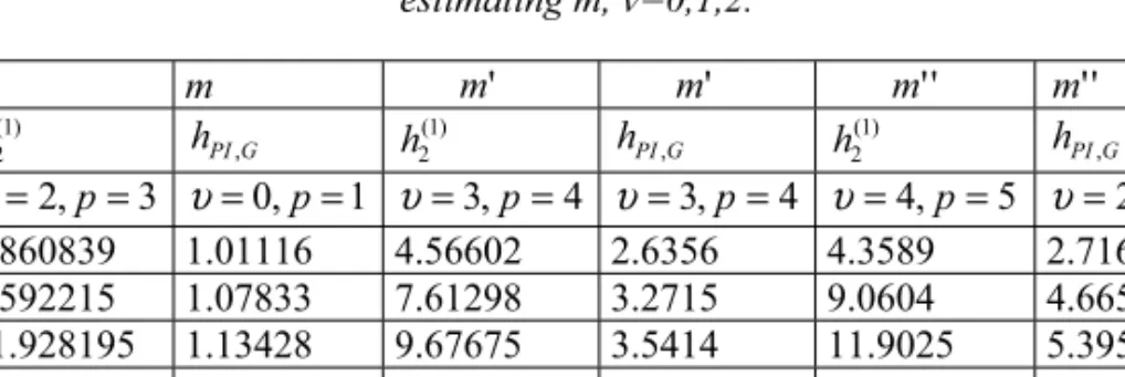
Table 1. Pilot and final bandwidths of the two stage global plug-in procedure for estimating m, Ȟ=0,1,2.

m m m' m' m'' m''

) 0 ( 2

h h2(1) hPI,G

) 1 ( 2

h hPI,G

) 1 ( 2

h hPI,G

3 ,

2 =

= p

υ υ=0,p=1 υ=3,p=4 υ=3,p=4 υ=4,p=5 υ=2,p=3 10 6.860839 1.01116 4.56602 2.6356 4.3589 2.7163 20 9.592215 1.07833 7.61298 3.2715 9.0604 4.6653 30 11.928195 1.13428 9.67675 3.5414 11.9025 5.3950 40 14.038808 1.18431 11.5646 3.7621 13.7104 5.7591 50 16.379445 1.23940 12.8962 3.9113 16.0595 6.2005 100 26.760712 1.47904 22.5909 4.9377 28.3775 8.3594

Having these bandwidths in mind Table 2 contains the proposed choices for the pilot bandwidth h₁ and the prepilot bandwidth (0)

2

Table 2. Values suggested for C₁,C₂,h₁ and (0) 2

h for estimating m . υ

Ȟ 0 1 2

1

C 24 24 24

2

C 64 52 51

1

h

5 1 1

−

n

Cδ 5

1 1

−

n

Cδ 5

1 1

−

n Cδ

) 0 ( 2

h ₉1

2 −

n

Cδ 11

1 2

−

n

Cδ 13

1 2

−

n Cδ

1.3.4. Computational issues

One of the problems that may appear in practice when using the local polynomial estimator is the fact that the matrix XtWX _{is singular or close to be}

singular. This occurs very often when the kernel has compact support, the design is equispaced and the bandwidth is small. Let consider a fixed point, x₀, where the estimation will be performed using a bandwidth h. Assume that the support of the kernel is [-1,1], then only the x_i's falling in the interval [x₀-h, x₀ +h] will be used to obtain the value of the estimator at x₀. Seifert and Gasser [26] have studied the case det(XtWX)=0 as well as conditions for finite variance of the local polynomial estimator reaching to the following conclusions.

1. Estimation at the point x₀ requires, at least, p+1 points in the interval [x₀-h, 0

x +h]. This condition is more and more restrictive as p increases.

2. In order to warranty that the variance of the estimator is finite, at least p+3 data points should fall within the interval [x₀-h, x₀ +h].

For both reasons whenever the final two-stage plug-in bandwidth or any auxiliary bandwidth is not large enough such that the interval interval [x₀-h, x₀ +h] containsp+3 points, the bandwidth is increased up to a value that meets this condition.

Along this unit, both the plug-in local and global bandwidth selectors have been considered. However, sometimes the global bandwidth may suffer of numerical problems, as those mentioned above, in the boundary of the support. In such cases, the global bandwidth has turned to be a local one in the boundary. In principle, the local plug-in bandwidth seems to be a more accurate smoothing parameter for estimating the regression derivatives in a grid of points. However it is clear that the algorithm becomes computationally much more time consuming.

It is evident that using a single smoothing parameter instead of a different one for every point in a grid makes a difference in terms of computations. However, there are some aspects that make the global bandwidth algorithm even much more efficient for an equispaced design. In that case, the matrix

(

)

change when x∈

(

)

(

)

[ ]

= h δ

l and u=n−

[ ]

(

)

has to be explicitly computed at every different point.

In order to save calculations for computing the estimators at the point x=xp, let

us write the (i,j)-th element of the matrix

(

)

or equivalently:

[

]

By defining the indices

»¼

It is clear that these implementation reduces the number of calculations for computing the estimator at a given point from O(n) to O((h/į)). This reduction is specially important for moderate bandwidths. In practice, for many of the thermogravimetric data sets we used, the computer time could be reduced by a factor of 10 to 20.

1.4. Conclusions

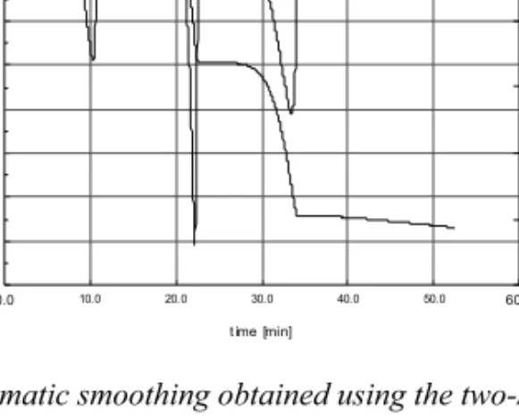
In this section we include the results obtained using the local polynomial estimator with two-stage plug-in bandwidth with covariances sum estimated for a sample of calcium oxalate. For comparison purposes we show the results obtained, for the same sample, using one of the smoothing routines incorporated to one of the standard software packages in calorimetry, the RSI Orchestrator.

0.0 10.0 20.0 30.0 40.0 50.0 60.0 -1.6

-1.4 -1.2 -1.0 -0.8 -0.6 -0.4 -0.2 0.0

0.2

2.0

3.0 4.0 5.0 6.0 7.0

8.0

t ime [min]

D

_

1W

/dt (

)

[

]

W

e

ig

h

t (

)

[m

g]

calcium oxalate_1

Figure 2. The automatic smoothing obtained using the two-stage global plug-in bandwidth.

2. Kinetic study using the logistic model regression 2.1. Introduction

TG is widely used to determine kinetic parameters for polymer decomposition. Both isothermal and dynamic heating experiments can be used to evaluate kinetic parameters. Each has advantages and disadvantages. In dynamic thermogravimetric analysis (TGA), the mass of the sample is continuously monitored while the sample is subjected, in a controlled atmosphere, to a thermal program, where the temperature is ramped at a constant heating rate. Ideally, a single thermogram has been said to be equivalent to a very large family of comparable isothermal volatilization curves and, as such, constitutes a rich source of kinetic data for volatilization [2].

The classical way to study the kinetics of these processes by TGA starts from the assumption that the weight loss follows the Arrhenius equation:

¸ ¹ · ¨ ©

§₋

⋅ =

RT E A

T

k( ) exp (17) where k, the reaction rate depends on the temperature, T. E, the activation energy may be considered constant in each degradation process (that appears as a clear step in the mass trace) since the degradation mechanism is supposed not to change in a narrow range of temperatures. A is another constant that, in the case that the kinetics follow a reaction order model, may be calculated from A=mtn, where n is the reaction order.

2.2. Other models

Many other models start from the Arrhenius equation, modified by Sesták-Berggren [3]:

(

)

[

(

)

]

m k dt d

α α

α

α _{= ( ) 1− −ln1−}

There are also some integrable models, like Ozawa [19], Flyn [8] and the one proposed by Popescu, C. [20], that allows for calculation of n and A from TGA data obtained at several heating rates. The method proposed by Conesa [6] considers that some organic fractions of the sample decompose independently giving an organic residue and an inorganic fraction. This model gave good correlation with the weight loss derivative data for different rubbers [10]. The method proposed by Carrasco F. and Costa J. [3] has been successfully applied to the thermal dagradation of polystyron. Although the application of these models to specific cases has been checked by detailed statistical studies, all of them are based on the Arrhenius equation and can not be generally applied to material degradations following very different kinetics. Moreover, its methodology is sometimes unease.

It has been said for methods based on one simple heating rate that quite different reaction models fit the data equally well (from the statistical point of view) whereas the numerical values of the corresponding Arrhenius parameters crucially differ (Vyazovkin [29]). Its physical meaning is obscure and no predictions can be done outside the range of experimental temperature (Vyazovkin). Other authors deemed the Arrhenius model inadecuate for the calculation of kinetic parameters from non-isothermal thermogravimetric curves [13]. Moreover, arising from the Kinetics Workshop, held during the 11th International Congress on Thermal Analysis and Calorimetry (ICTAC) in Philadelphia, USA, in 1996, sets of kinetic data were prepared and distributed to volunteer participants for their analysis using any, or several, methods they wished. The results obtained by each researcher were different than the ones obtained by the others, Brown, M. et al. [2]. All of this confirms our believing that the existing models cannot be generally applied and sometimes it is not clear which one is the best suitable to each case. That is the reason to propose an alternative model that will be described in the following sections.

2.3. Logistic model proposed

This model proposes to decompose the TGA trace in several logistic functions, assuming that each of the functions represents the degradation kinetics of each component of the sample. Even in the case of homogeneous materials, it is supposed that several different structures may exist, each one following its specific kinetics that may be different from the others. In this model, it is assumed that a TGA trace may be fitted by a combination of logistic functions:

(

)

t t k

i

i i i

e e t f

t b a f w t Y

+ =

+

=

_¦

=

1 ) (

) (

1

(17) where i=1,2,,k represent different components from the weight loss process point of view, not necessarily different chemical compounds.

sample and the Y_i(t) functions have to tend to the mass of each component in the original sample, that is, the wi(t)constants correspond to the weight loss of the sample in each weight loss process. These weight loss processes generally appear as clear steps of the TGA trace.

The function Y(t)that represents the overall TGA trace may be expressed as a sum of Y_i(t) functions like this:

(

)

f w t

Y_i()= _{i i} + _i

The constansts a_i and b_i are calculated taking into account that the b_i values represent the slope of the weight steps while the change of scale comes from the ai/bi

rates. The w_i values mean the weight of each component in the sample.

0 2 4 6 8 10 12 14 16

5 10_t 15 20

Figure 3. Function obtained from the sum of 4 simple logistic functions.

) 16 ( ) 5 43 ( 7 ) 2 14 ( 4 ) 4 12 ( 5 )

(t f t f t f t f t

g = − + − + − + −

2.3.1. Kinetic study using the logistic model

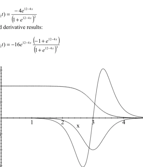
Once the regression function of the TGA trace was obtained, it is inmediate to obtain derivatives. Thus, for example, the first derivative of the TGA trace (DTG), which is used by many kinetic models since it represents the weight loss rate along the time, may be expressed by the following equation (18):

(

)

( )

' )

(

t t k

i

i i i i

e e t f

t b a f b w t dTGA

+ =

+

=

_¦

=

Analyzing, for example, its first component, i=1,

x x

e e t b a

f _{12 4}

4 12 1 1

1 )

( ₋

−

+ = +

Its first derivative is:

(

)

1

1 4 ) ( '

x x

e e t

b a f

− −

+ − = +

Its second derivative results:

(

)

(

)

12 1

1

1 1 16

) ( '

x x x

e e e

t b a f

− − −

+ + − −

= +

-1.5 -1 -0.5 0 0.5 1 1.5

1 2 3 4 5

x

Figure 4. The plots of the f function and its first and second derivatives are shown.

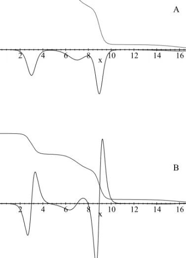
Other possible interpretation of the logistic parameters is obtained aplying a change of scale and position. It improves equation (18) since the new values show the weight loss rate b' and the exact position in the time axis of the point corresponding to i

the half weight loss of each step a' : _i

¸¸ ¹ · ¨¨ ©

§ −

=

i i i i

b a t f w t Y

' ' )

( (19)

-5 0 5 10 15

2 4 6 8 10 12 14 16 18

x

-15 -10 -5 0 5 10 15

2 4 6 8 10 12 14 16 18

x

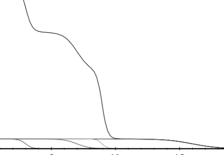
Figure 5. The overall function, obtained from the sum of the 4 functions previously described (dashed curve) and the first (A) and second (B) derivatives.

2.3.2. Logistic parametric fitting

For the fitting of data to a logistic function it is needed the calculation of values for the equation parameters. This task is usually performed by using a statistical software. In this case, the non linear regression and derivatives packages of the S-plus software.

The algorithm used for the non linear regression is:

n i

x m

y_i = ( _i,θ)+ε_i, =1,2,,

A

where the response variable and the independent variable values are represented by y_i

and xi, respectively. θ is the parameters vector, that is estimated by least squares and i

ε are the errors, with normal distribution, mean zero and constant variance. The residuals of the model are defined as:

n

The parameters of the model were estimated by the non linear least squares method. The fundamentals of this method were described by Gay, D. M. [14]

The Levenberg-Marquart method routine for generation of the approximation sequence to the minimum point, based in the “trust region” algorithm, was used for the calculation of the parameter values that minimize that sum. This algorithm was discussed by Chambers, J. M., and Hastie, T. J. [4] . Its application to the computer calculation was described Dennis, J. E. et al. [7].

One of the problems that appear when fitting is to choose some statarting points for the different parameters to estimate. To do this, one possibility consists in, by observation of the TGA trace, to try to estimate the inflexion. Since this method is not easy and requires previous expertise, we propose a method based in the idea of supposing that the data follow a logistic regression (Equation 3). So it is possible to fit the logit Y(t)/w function to a straight line which y origin is ai and which slope isbi.

The reason for this linear fitting is explained as follows:

(

)

_{( )}

2.3.3. Application of the logistic regression to different cases

In order to validate the model in extreme situations, some TGA experiments exhibiting very different behaviours were considered. The first one corresponds to the hexahydrophtalic anhydride that underwent a typical evaporative process. It consisted in a single weight loss step with maximum weight loss rate at the end of the step [18]. The second one corresponds to the analysis of wood from Eucaliptus globulus. The wood is a very complex material where the main components are cellulose and lignin. Its thermal behaviour is quite complex and overlapped processes seem to be involved. Apparently, it decomposes in four main steps. Other complex cases considered were wood from Cupressus sempervirens and plasticized poly-(vinyl chloride).

Hexahydrophtalic anhydride case

In the case of a hexahydrophtalic anhydride experiment, since there is only one weight loss step, only one logistic function is needed to modelise the TGA trace. In other words, the equation that describes the overall process is

(

)

wf t

The lineal fitting of Equation (7) to the TGA data, by least squares, gives the values for the a and b parameters, resulting the following expression that describes the behaviour of the hexahydrophtalic anhydride in that experiment:

) 024 . 0 48 . 17 exp( 1

) 024 . 0 48 . 17 exp( 93 . 12 ) (

t t t

Y

− +

− =

Time

Weigth

0 100 200 300 400 500 600 700 800

234

56

78

9

1

0

1

1

1

2

1

3

Figure 6. TGA trace obtained from a hexahydrophtalic anhydride experiment.

The case of cupressus wood

x

y

0 400 800 1200 1600 2000 2400 2800 3200 3600 4000 4400 4800

0

5

15

25

35

45

55

65

75

85

95

Linear fitting of different parts of the curve were performed in order to find the parameter values:

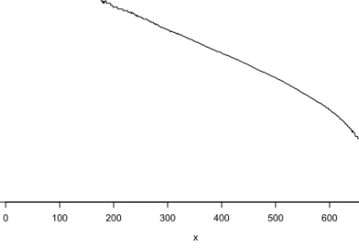
In order to do this, the logit(y) function is plotted versus x and a line is fitted by the S-Plus software:

x

logit(y)

0 100 200 300 400 500 600 700

-5

-4

-3

-2

-1

0123

45

Figure 8. Plot of the logit (y) function versus time in the range from 0 to 700 s.

The fitting was performed in two ranges of data. The first one is [0:700]. Since the neighbour values to 0 and 700 result in log 0, ten points will be suppresses in each end of the range. A line was fitted between 10 and 690, resulting in w1=8.5, a1=5.12, b1=0.012. These values were used to initiate the model.

The next range [700:1640], that includes a step, was operated in the same way, resulting the following values a2=9.175879, b2=-0.004551135 with 1631 total degrees of freedom and residual standard error= 0.7296343

Finally, the model was fitted with these starting values.

Parameter Value Std. Error t value

w1 10.53520 0.0995712 105.8060

a1 3.79104 0.1033680 36.6750

b1 -0.00765 0.0001785 42.8834

w2 89.90570 0.0350401 2565.7900

a2 12.63650 0.0331148 381.5970

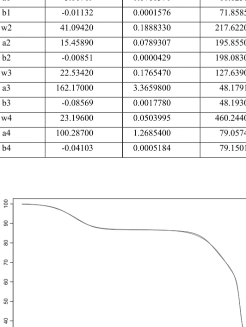
Fitting for the eucaliptus experiment

In this case four logistic components were assumed:

In this case, the fitting to obtain the starting values was performed in four ranges, giving the following values for the parameters of the model:

Parameter value Std. Error t value

w1 13.04790 0.0579730 225.0690

a1 5.06769 0.0766370 66.1258

b1 -0.01132 0.0001576 71.8585

w2 41.09420 0.1888330 217.6220

a2 15.45890 0.0789307 195.8550

b2 -0.00851 0.0000429 198.0830

w3 22.53420 0.1765470 127.6390

a3 162.17000 3.3659800 48.1791

b3 -0.08569 0.0017780 48.1930

w4 23.19600 0.0503995 460.2440

a4 100.28700 1.2685400 79.0574

b4 -0.04103 0.0005184 79.1501

Time

Weigth

0 200 400 600 800 1000 1200 1400 1600 1800 2000

30

40

50

60

70

80

90

100

Fitting in the case of PVC

In this case the fitting to obtain the starting values was performed in four ranges, resulting in the following equation:

Time

Weigth

0 500 1000 1500 2000 2500 3000 3500

02468

1

0

1

2

1

4

1

6

Figure 10. Fitting in the case of PVC.

) 75 . 2 69 . 36 ( 86 . 6 ) 09 . 2 47 . 22 ( 061 . 3 ) 15 . 2 45 . 14 ( 276 . 5 ) 09 . 0 631 . 0 ( 287 .

2 f − t + f − t + f − t + f − t

2.3.4. Physical meaning of the parameters

Once the fittings were performed in different cases it is clear that the w_i(t) values represent the magnitude of each weight loss process. The b_i parameters have the meaning of sample volatilization rate, while the a_i value represents the scale.

2.4. Conclusions

1. This method allows for including at once the overall trace from a TGA experiment, while the classical methods can only be applied to a single step each time.

2. Overlapped degradation processes can be explained by this method. Since the existing models were thought to explain single processes, they generally fit very badly to overlapped processes.

3. It explains the thermal degradation of each component of the sample by a single function that may be easily understood from the physical point of view.

4. This model shows the contribution of each single degradation process to the overall process. It is very useful in order to improve thermal stability of materials.

5. It allows for measuring the statistical goodness of the fitting by signification contrast.

7. It is easier to apply the classical kinetic models on the functions obtained by our method than on the row TGA data, since the row data contents noise that affect the derivative and integral estimations. In whose classical methods are based.

8. The asymptoticity is perfectly reproduced at the beginning and end of each degradative process.

3. Functional non-parametric model for materials discrimination by thermal analysis

3.1. Introduction

An important topic in Material Science is the classification of materials. The information obtained by thermo gravimetric analysis can be used to this aim. In this work, functional regression by nonparametric methods was used for the classification of different polymers. The method can be extended to any kind of material that can be analyzed by TGA.

Pattern recognition techniques deal with classification of observations in a finite number of classes (Watanabe, [30]).

It can be done by several parametric models, such as the discriminant analysis. Nevertheless, in the case of curves, the problem is functional and non parametric models are more suitable, since they take into account all the information from the sample (Ramsay and Silverman, [22]).

The method of classification proposed in this work is based in functional regression by nonparametric methods. Several PVC and wood samples were classified by this method. Finaly, many simulated experiments were used to evaluate the accuracy of the method.

3.2. Nonparametric classification method

The nonparametric methods do not require previous estimation of any parameter. In this case, the kernel method was chosen. It is a nonparametric discrimination method that has been proved to work well in many cases (Ferraty and Vieu, [11]).

The nonparametric Bayes clasification rule was used to classify the sample. It assigns a future observation to the highest probability class.

The different TGA curves, X_i, were taken as explanatory variable X_i, and the classes a sample of the response Y_i.

Considering a new TGA curve, obtained from a material to classify, the estimator of the posterior probability is given by:

{ }

¦

¦

= = =

¸ ¸ ¹ · ¨

¨ ©

§ −

¸ ¸ ¹ · ¨

¨ ©

§ −

=

n

i

i n

i

i j

Y j

h X x K

h X x K x

r

i

h

1 1

1 ) (

ˆ (20)

Equation (20) is a versión of the Nadaraya-Watson estimator reported by Ferraty and Vieu, [11].

The L₁ norm will be used as distance between curves and h is the bandwidth, or smoothing parameter.

{ }

ˆ max arg )

( j

h G j

h x r

d

≤ ≤

=

where rˆh(j) represents the estimation of the probability of the sample belonging to the j

class.

The parameter smoothing h will be chosen that minimizes the probability of misclassifying a future observation. This bandwidth parameter will be taken as h_CV, that minimizes the following cross-validation function:

{ }

¦

= ≠ −

−

= n

i Y d Xi

i h i n h CV

1 ( )

1 ₁

)

( where i

h

d− is the classification rule, built up without the i-th observation.

Finally, given a new sample and its TGA trace, denoted as x, the distances from this trace to the others will be calculated and ()

ˆhj

r will be estimated for each class of material j∈

{

}

). ( ˆ() x r j

h

3.3. Application to PVC samples

The method of classification proposed was applied to a sample of 16 PVC items, plasticized in different degrees. The sample weight was about 35 mg in all the cases. The TGA experiment consisted in a heating ramp from 25 to 600 ºC at 10 K/min followed by an isothermal step at 600 ºC for 15 minutes. A 50 ml/min purge of air was kept along the experiment.

20.0 21.875 23.75 25.625 27.5 29.375 31.25 33.125 35.0 35.0

41.818 48.636 55.455 62.273 69.091 75.909 82.727 89.545 96.364 103.18

110.0

time [min]

W

tP

e

rc

ent

(

)

[%

]

0.0 10.0 20.0 30.0 40.0 50.0 60.0 70.0 80.0

Figure 12. Overlay of two TGA traces, obtained from different samples of PVC.

Each sample was classified by keeping itself excluded from the reference population. A 99.4 % of correct classification was obtained by the application of the method proposed to the 16 PVC samples. It can be seen in Figure 13, which plots the cross-validation function.

3.4. Simulated experiments

A simulation study was performed in order to check the method. Three kinds of wood were chosen, since these materials are very much alike in composition and thermal behaviour. It is not easy to classify this kind of materials only by TGA experiments. From actual experiments of the three samples, two sets of experiments were simulated by a logistic mixture model. The simulation was performed for each of the three groups, using the function:

.)

The parameters for the model were simulated following a k_r-dimension Normal distribution. Two different situations were considered: parameters being independent and dependent.

h

The first set of simulated experiments consisted of 90 TGA traces, whose probability to belong to each of the three groups was 1/3. The cross-validation bandwidth and the minimum of the cross-validation function were obtained from that simulated traces.

Then, a second set of 1000 traces was simulated, using the same probability than in the first set. Each curve was classified by the estimated non parametric rule of Bayes. The result of the classification was compared with the group from wich the trace was simulated. The percent of the 1000 traces that were correctly classified was taken as an estimation of the probability of correct classification. The results show that the lower the varianze of the model the langer the percent of correct classification, reaching 92 to 95 % correct classification for varianzes with values of 1/8 of the original varianze. Generally, the percent of correct classification slightly increases in case of dependent data.

References

1. Arnold M., Veress G. E., Paulik J., Paulik F. (1982). A critical reflection upon the application of the Arrhenius model to non-isothermal thermogravimetric curves. Thermochimica Acta; 52: 67-81.

2. Brown M.E., Maciejewski M.,Vyazovkin S., Nomen R., Sempere J., Burnham A., Opfermann J., Strey R., Anderson H.L., Kemmler A., Keuleers R., Janssens J., Desseyn H.O., Chao L., Tong B., Roduit B., Malek J. and Mitsuhashi T. (2000). Computational aspects of kinetic análisis. Thermochimica Acta; 355: 125-143. 3. Carrasco F. and Costa J. (1989). Modelo Cinético de la descomposición térmica del

poliestireno.Ingeniería Química; 121-129.

4. Chambers J. M. and Hastie T. J. (1992). Statistical Models in S. Pacific Grove, CA Wadsworth and Brooks, Chapter 10.

5. Cleveland, W. S. (1979). Robust locally weighted regression and smoothing scatterplots. Journal of the American Statistical Association, 74, 829-836.

6. Conesa J. A., Marcilla A. (1996). Kinetic study of the thermogravimetric behavior of different rubbers. Journal of Analytical and Applied Pyrolysis;37: 95-110. 7. Dennis J. E., Gay D. M. and Welsch R. E. An Adaptive Nonlinear Least-Squares

Algorithm ACM Transactions on Mathematical Software, Springer, Berlin 1981, 348-368.

8. Doyle C. D. (1961). Kinetic analysis of thermogravimetric data. Journal of Applied Polymer Science; 15, 285-292.

9. Fan, J. and Gijbels, I. (1995). Data-driven bandwidth selection in local polynomial fitting: variable bandwidth and spatial adaptation. Journal of the Royal Statistical Society, Series B, 57, 2, 371-394.

10. Fan, J. and Gijbels, I. (1996). Local polynomial modelling and its applications. Chapman and Hall. London.

11. Ferraty, F. and Vieu P. (2002). The functional nonparametric model and application to spectrometric data. Computational Statistical, 17, (4). 545-564.

12. Flynn J. H.,Wall L. A., Quick A. (1966). Direct Method for the Determination of Activation Energy from Thermogravimetric Data. Polymer Letters;4: 323-328 13. Francisco, M. and Vilar-Fernández, J. (2001). Local polynomial regression

14. Freeman B. and Carroll B. (1958). The application of thermoanalytical techniques to reaction kinetics. The thermogravimetric evaluation of the kinetic of the decomposition of calcium oxalate monhydrate. Journal of Physical Chemistry;62: 394-397.

15. Friedman H. L. (1964). Kinetics of thermal degradation of char forming plastics from thermogravimetry. Application to a phenolic plastic. Journal of Polymer Science; Part C, 6: 183-195.

16. Gasser,T. and Müller, H.G. (1979). Kernel estimation of regression functions. In Smoothing techniques for curve estimation, Lecture Notes in Mathematics, 757, 23--68. Springer-Verlag.

17. Gay D. M. (1984). A trust region approach to linearly constrained optimization in Numerical Analysis. Springer, Berlin, 171-189.

18. Nadaraya, E. A. (1964). Remarks on nonparametric for density functions and regression curves. Theory of Probability and its Applications. 15, 134-137.

19. Ozawa T. (1965). A New Method of Analyzing Thermogravimetric Data. Bulletin of the Chemical Society of Japan;38: 1881-1886

20. Popescu, C. (1984). Variation of the maximum rateo f conversión and temperatura with heating rate in non-isothermal kinetics. Thermochimica Acta;82: 387-389. 21. Priestley, M. B. and Chao, M. T. (1972). Nonparametric function fitting, Journal of

the Royal Statistical Society, Series B, 34, 385-92.

22. Ramsay, J. and Silverman, B. (1997). Functional Data Analysis. Springer-Verlag, New York.

23. Ruppert, D. and Wand, P. (1994). Multivariate locally weighted least squares regression. The Annals of Statistics, 22, 1346-1370.

24. Ruppert, D., Sheather, S. J. and Wand, M. P. (1995). An effective bandwidth selector for local least squares regression. Journal of the American Statistical Association, 90, 1257-1267.

25. Savitzky, A. and Golay, M. (1964). Smoothing and Differentiation of Data by Simplified Least Squares Procedures. Analytical Chemistry. 36, 1627-1639. 26. Seifert, B. and Gasser T. (1996). Finite sample variance of local polynomials:

analysis and solutions. Journal of the American Statistical Association, 91, 267-275. 27. Sestak, J. and Berggren, G. (1971) Study of the kinetics of the mechanism of

solid-state reactions at increasing temperatures. Thermochimica Acta, 3, 1-12.

28. Stone, C.J. (1977). Consistent nonparametric regression. The Annals of Statistics, 5, 595-620.

29. Vyazovkin, S. (1996). A unified approach to kinetic processing of nonisothermal data. International Journal of Chemical Kinetics, 28, 95-101.

30. Watanabe, S. (1985). Pattern Recognition. Human and Mechanical. Wiley, New York.