TítuloNew approaches to quantification and management of model risk

Texto completo

(1)P H D. THESIS New Approaches to Quantification and Management of Model Risk. AUTHOR: Zuzana Krajčovičová D IRECTORS: Pedro Pablo Pérez Velasco Carlos Vázquez Cendón. TESE PRESENTADA PARA A OBTENCIÓN DO TÍTULO DE DOUTOR NA UNIVERSIDADE DA CORUÑA DEPARTAMENTO DE MATEMÁTICAS FACULTADE DE INFORMÁTICA, A CORUÑA (SPAIN) July, 2018.

(2)

(3)

(4)

(5) Funding This research has been funded by the following project: • MSCA-ITN-EID - European Industrial Doctorates (WAKEUPCALL Grant Agreement 643045) Funded under: H2020–EU.1.3.1. – Fostering new skills by means of excellent initial training of researchers.

(6)

(7) To all whose stayed on my side..

(8)

(9) Acknowledgements ”The secret to creativity is knowing how to hide your sources.” (Albert Einstein). The work presented in this doctoral thesis has been carried out under the Horizon 2020 EU Programe for Research and Innovation (European Industrial Doctorates) with the joint supervision of Universidade da Coruña (UDC) and Banco Santander. This research would not have been possible without the financial support provided by H2020–EU.1.3.1. Marie Sklodowska–Curie Innovative Training Networks and to Banco Santander during my two–year stay in Madrid. A doctoral thesis is often described as a solitary endeavour, though the long list that follows definitely proves the opposite. To all these people, who contributed to the research in their own particular way, I owe my gratitude and thanks. I would like to express my appreciation to my supervisor Carlos Vázquez Cendón at the UDC for his suggestions and revisions of the work but also for handling all the arrangements necessary regarding the project. I thank him for providing me with the opportunity to participate on this project. My sincere and very special thanks go to my supervisor Pedro Pablo Pérez Velasco (Model Risk area, Head of the Non–Financial Validation Unit) at Banco Santander who kept a sense of humour and motivation when I had lost mine. I owe my deep gratitude for his friendly and stimulating guidance and care, invaluable suggestions, keen interest, constructive criticisms and constant encouragement throughout all the stages of the work, for going far more beyond the call of duty. His willingness to share his time (even at the cost of cold tea), intellect (that shaped my thinking and navigated my chaos) and immense (and evergrowing) patience is the major reason this dissertation was completed. ”It is the supreme art of the teacher to awaken joy in creative expression and knowledge.” (Albert Einstein) A special thanks also goes to José Luis Fernández Pérez (Universidad Autonoma de Madrid) for his interest, guidance, support and willingness to help, especially at the early stages of my research. Along with my above mentioned supervisors, the experts from Banco Santander in Madrid, where I have conducted most of the work, were of outstanding importance to my research. My very special thanks goes to Eneas Nebayot Calderón González (Model Risk department, Governance and Control area) for his selfless time, effort and inspiring enthusiasm in sharing his knowledge and introducing me to his field of expertise. I am grateful to Inmaculada González Peréz, José Carlos Colas Fuentes and Olivia Peraita Ezcurra from the Credit Risk models validation area for providing insight and feedback that greatly assisted the example presented in Chapter 7. To Luis Alberto Herraiz Garrote (Trader, Executive Director) and Álvaro Iglesias Barbero (IR quant analyst) for sharing.

(10) their knowledge, insight and suggestions that helped to shape the contribution presented in Chapter 9. I extend my many thanks to many other people from Model Risk department, with special recognition to Esther Fernández Martı́n (Non–Financial Validation), Ruth Manso Dı́az (Internal Validation) and Javier López Ibáñez (Market risk Validation) for providing insights into their areas of expertise, practical suggestions and willingness to share their time and unparalleled knowledge. A journey is easier when we travel together. Interdependence is certainly more valuable than independence. Special thanks to all my fellow PhD colleagues in the project, Anastasia Igorevna Borovykh, Andrea Fontanari, Enrico Ferri, Ki Wai Chau and Sidy Diop for their support, fruitful discussions, shared frustrations and encouragement. As my supervisor once said, if you want to emphasize an important point put it at the end. On that account, last, but not least, I would like to thank my family and Suren that had to learn to accept my separation from them and still gave me nothing but support, love and encouragement: my love and gratitude for them can hardly be expressed in words.. I find that a great part of what I have gained from the project, was acquired by expecting something and finding something else, much more valuable, on the way.. 10.

(11) Contents I. C APITAL AND R ISK M ANAGEMENT M ODELS. 29. 1. C APITAL MANAGEMENT. 39. 1.1. R EGULATORY CAPITAL . . . . . . . . . . . . . . . . . . . . . . . . . . . . . . . . . . . . . . . .. 41. 1.1.1. C APITAL ADEQUACY REQUIREMENTS . . . . . . . . . . . . . . . . . . . . . . . . . . . .. 49. 1.2. E CONOMIC CAPITAL . . . . . . . . . . . . . . . . . . . . . . . . . . . . . . . . . . . . . . . . . .. 52. 1.3. C ONCLUSIONS . . . . . . . . . . . . . . . . . . . . . . . . . . . . . . . . . . . . . . . . . . . . .. 59. 2. C REDIT AND M ARKET R ISKS. 61. 2.1. C REDIT R ISK . . . . . . . . . . . . . . . . . . . . . . . . . . . . . . . . . . . . . . . . . . . . . .. 61. 2.1.1. P ROBABILITY OF D EFAULT M ODELS . . . . . . . . . . . . . . . . . . . . . . . . . . . . .. 64. 2.1.2. L OSS G IVEN D EFAULT M ODELS . . . . . . . . . . . . . . . . . . . . . . . . . . . . . . .. 65. 2.1.3. E XPOSURE AT D EFAULT M ODELS . . . . . . . . . . . . . . . . . . . . . . . . . . . . . .. 66. 2.1.4. M AIN SOURCES OF M ODEL RISK . . . . . . . . . . . . . . . . . . . . . . . . . . . . . . .. 68. M ARKET R ISK (T RADING ) . . . . . . . . . . . . . . . . . . . . . . . . . . . . . . . . . . . . . .. 69. 2.2.1. DATA , M ODELS AND M ETHODOLOGIES . . . . . . . . . . . . . . . . . . . . . . . . . . .. 70. 2.2.2. M AIN S OURCES OF M ODEL RISK . . . . . . . . . . . . . . . . . . . . . . . . . . . . . . .. 75. F INANCIAL D ERIVATIVES . . . . . . . . . . . . . . . . . . . . . . . . . . . . . . . . . . . . . . .. 76. 2.3.1. DATA , M ODELS AND M ETHODOLOGIES . . . . . . . . . . . . . . . . . . . . . . . . . . .. 77. 2.3.2. R ISKS ASSOCIATED WITH F INANCIAL D ERIVATIVES . . . . . . . . . . . . . . . . . . . .. 80. 2.3.3. M AIN S OURCES OF M ODEL R ISK . . . . . . . . . . . . . . . . . . . . . . . . . . . . . .. 83. S TRUCTURAL AND BALANCE SHEET RISK . . . . . . . . . . . . . . . . . . . . . . . . . . . . . .. 84. 2.4.1. L IQUIDITY R ISK . . . . . . . . . . . . . . . . . . . . . . . . . . . . . . . . . . . . . . . .. 85. 2.4.2. I NTEREST R ATE R ISK ON T HE BANKING B OOK . . . . . . . . . . . . . . . . . . . . . .. 88. 2.4.3. FX S TRUCTURAL RISK . . . . . . . . . . . . . . . . . . . . . . . . . . . . . . . . . . . .. 90. 2.4.4. M AIN S OURCES OF M ODEL R ISK . . . . . . . . . . . . . . . . . . . . . . . . . . . . . .. 91. 2.2. 2.3. 2.4. 1.

(12) 3. N ON –F INANCIAL R ISKS. 93. 3.1. O PERATIONAL R ISK . . . . . . . . . . . . . . . . . . . . . . . . . . . . . . . . . . . . . . . . . .. 94. 3.1.1. DATA , M ODELS AND M ETHODOLOGIES . . . . . . . . . . . . . . . . . . . . . . . . . . .. 96. 3.1.2. M AIN S OURCES OF M ODEL R ISK . . . . . . . . . . . . . . . . . . . . . . . . . . . . . . 100. 3.2. OTHER N ON –F INANCIAL R ISKS . . . . . . . . . . . . . . . . . . . . . . . . . . . . . . . . . . . 100 3.2.1. 4. P ROVISIONS , S TRESS T ESTING AND D EPENDENCIES 4.1. 4.2. 4.3. 105. P ROVISIONS . . . . . . . . . . . . . . . . . . . . . . . . . . . . . . . . . . . . . . . . . . . . . . 105 4.1.1. DATA , M ODELS AND M ETHODOLOGIES . . . . . . . . . . . . . . . . . . . . . . . . . . . 106. 4.1.2. M AIN S OURCES OF M ODEL R ISK . . . . . . . . . . . . . . . . . . . . . . . . . . . . . . 108. S TRESS T ESTING . . . . . . . . . . . . . . . . . . . . . . . . . . . . . . . . . . . . . . . . . . . . 110 4.2.1. DATA , M ODELS AND M ETHODOLOGIES . . . . . . . . . . . . . . . . . . . . . . . . . . . 110. I NTERRELATIONSHIPS B ETWEEN D IFFERENT T YPES OF R ISK . . . . . . . . . . . . . . . . . . . 112 4.3.1. II. C ONCLUSIONS . . . . . . . . . . . . . . . . . . . . . . . . . . . . . . . . . . . . . . . . . 103. M AIN S OURCES OF M ODEL R ISK . . . . . . . . . . . . . . . . . . . . . . . . . . . . . . 115. M ODEL R ISK : M ANAGEMENT AND Q UANTIFICATION. 119. 5. I DENTIFICATION OF P OTENTIAL S OURCES OF M ODEL R ISK. 125. 6. A N EW A PPROACH TO Q UANTIFICATION OF M ODEL R ISK FOR P RACTITIONERS. 133. 6.1. BACKGROUND ON R IEMANNIAN G EOMETRY . . . . . . . . . . . . . . . . . . . . . . . . . . . . 135. 6.2. M ODELLING P ROCESS S TEPS AND Q UANTIFICATION OF M ODEL R ISK . . . . . . . . . . . . . . 137. 6.3. N EIGHBOURHOOD A ROUND THE M ODEL . . . . . . . . . . . . . . . . . . . . . . . . . . . . . . 139. 6.4. W EIGHT F UNCTION D EFINITION . . . . . . . . . . . . . . . . . . . . . . . . . . . . . . . . . . . 140 6.4.1. 7. Weight Function Construction . . . . . . . . . . . . . . . . . . . . . . . . . . . . . . . . . 142. 6.5. M EASURE OF M ODEL R ISK . . . . . . . . . . . . . . . . . . . . . . . . . . . . . . . . . . . . . . 146. 6.6. C ONCLUSIONS AND F URTHER R ESEARCH . . . . . . . . . . . . . . . . . . . . . . . . . . . . . . 148. A PPLICATION TO C APITAL C ALCULATION. 151. 7.1. PD MODEL (p0 ) . . . . . . . . . . . . . . . . . . . . . . . . . . . . . . . . . . . . . . . . . . . . . 152. 7.2. Q UANTIFICATION OF M ODEL R ISK . . . . . . . . . . . . . . . . . . . . . . . . . . . . . . . . . . 153 7.2.1. Identification of potential sources of model risk . . . . . . . . . . . . . . . . . . . . . . . . 155. 7.2.2. Choosing a suitable Riemannian metric . . . . . . . . . . . . . . . . . . . . . . . . . . . . 156 2.

(13) 8. 9. 7.2.3. Neighbourhood selection . . . . . . . . . . . . . . . . . . . . . . . . . . . . . . . . . . . . 156. 7.2.4. Choosing an appropriate weight function . . . . . . . . . . . . . . . . . . . . . . . . . . . 157. 7.2.5. Measure of Model Risk . . . . . . . . . . . . . . . . . . . . . . . . . . . . . . . . . . . . . 159. Q UANTIFICATION OF M ODEL R ISK : DATA U NCERTAINTY. 161. 8.1. S AMPLE S PACE AND F ITTING P ROCESS . . . . . . . . . . . . . . . . . . . . . . . . . . . . . . . 162. 8.2. C HOICE OF M ETRIC ON THE S AMPLE S PACE . . . . . . . . . . . . . . . . . . . . . . . . . . . . 165. 8.3. Q UANTIFICATION OF M ODEL R ISK ON THE S AMPLE S PACE . . . . . . . . . . . . . . . . . . . . 167. 8.4. C ONCLUSIONS AND F URTHER RESEARCH . . . . . . . . . . . . . . . . . . . . . . . . . . . . . . 169. M ODEL R ISK AND D IFFERENTIAL G EOMETRY A PPLIED TO S ENSITIVITY A NALYSIS. 171. 9.1. G EOMETRICAL BACKGROUND . . . . . . . . . . . . . . . . . . . . . . . . . . . . . . . . . . . . 172. 9.2. N EED TO CONSIDER NONLINEAR STRUCTURES . . . . . . . . . . . . . . . . . . . . . . . . . . . 174. 9.3. O PTION P RICE S ENSITIVITIES . . . . . . . . . . . . . . . . . . . . . . . . . . . . . . . . . . . . 175. 9.4. DAILY P&L ANALYSIS FOR D IGITAL OPTIONS UNDER THE B LACK –S CHOLES MODEL . . . . . . 177. 9.5. C HOICE OF A R IEMANNIAN METRIC . . . . . . . . . . . . . . . . . . . . . . . . . . . . . . . . . 181. 9.6. 9.7. 9.5.1. Fisher–Rao information metric . . . . . . . . . . . . . . . . . . . . . . . . . . . . . . . . . 182. 9.5.2. Christoffel symbols based on critical points of digital options . . . . . . . . . . . . . . . . . 185. OTHER A PPLICATIONS . . . . . . . . . . . . . . . . . . . . . . . . . . . . . . . . . . . . . . . . . 187 9.6.1. Digital Option on synthetic underlying asset following Heston model . . . . . . . . . . . . 187. 9.6.2. D IGITAL O PTION ON VOLATILITY I NDEX ON E QUITY . . . . . . . . . . . . . . . . . . . 192. C ONCLUSIONS AND F URTHER R ESEARCH . . . . . . . . . . . . . . . . . . . . . . . . . . . . . . 195. 10 C ONCLUSIONS AND F URTHER R ESEARCH. 197. 3.

(14) 4.

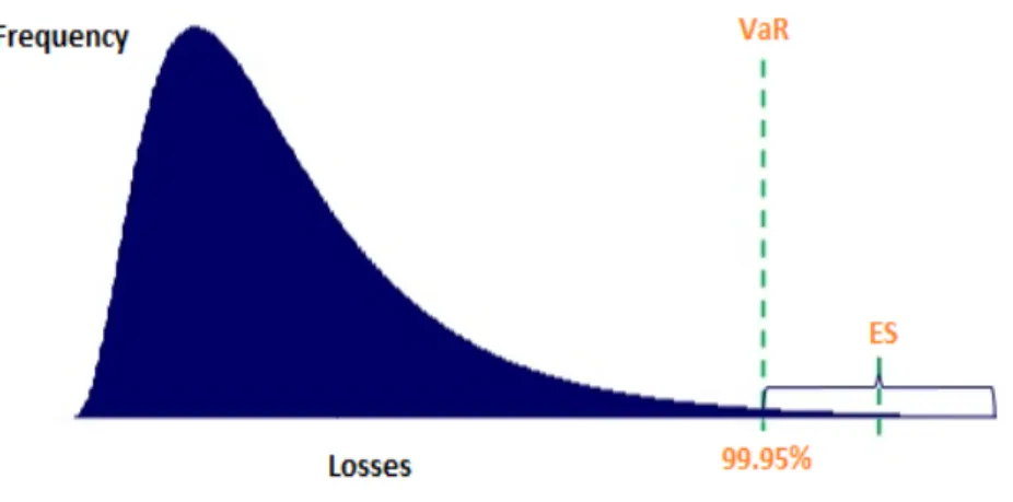
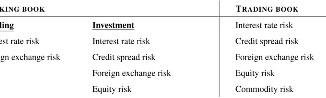
(15) List of Figures 1. Examples of models subject to governance and model risk management of a large global bank. . . .. 23. 2. The main areas and subareas of an effective MRM. . . . . . . . . . . . . . . . . . . . . . . . . . .. 25. 3. The structure of the four lines of defence model as proposed by FSI. . . . . . . . . . . . . . . . . .. 32. 4. Risk Taxonomy summarizing the main risk classes, including financial, non–financial risks and external market risks. For more details, we refer the reader to Chapters 2 for credit and market risks, to Chapter 3 for operational risks and other relevant economic capital inputs, and to Chapter 4 for other types of non–financial risk.. 1.1. . . . . . . . . . . . . . . . . . . . . . . . . . . . . . . . . . . .. 34. Figure captures how variation in realised losses over time leads to a distribution of losses for a financial institution. Note that EL does not necessarily equal to the historical loss experience as the portfolio components may change. . . . . . . . . . . . . . . . . . . . . . . . . . . . . . . . . . . .. 40. 1.2. Structure of Basel III Accord. Source: Moody’s Analytics . . . . . . . . . . . . . . . . . . . . . .. 45. 1.3. The diagram outlines how the Basel III minimum add–on, conservation buffer and counter–cyclical buffer affect the core, Tier 1 and Tier 1 + 2 ratios in comparison to Basel II. . . . . . . . . . . . . .. 47. 1.4. Types of risks included in Regulatory and Economic capital under Basel framework. . . . . . . . .. 53. 1.5. One of the approaches to derive EC (silo approach) is based on estimating a risk profile for each risk category and then combined to give an aggregate risk profile, from which an overall capital requirement is obtained by applying a risk metric to the risk profile. . . . . . . . . . . . . . . . . .. 54. 1.6. Comparison of two standard risk measures: Value–at–risk (VaR) and Expected Shortfall (ES). . . .. 55. 1.7. Loss distribution: Expected and Unexpected Loss. . . . . . . . . . . . . . . . . . . . . . . . . . . .. 56. 2.1. Asset value process in the Black–Scholes–Merton model. In this model, a default occurs whenever the asset value settles below the default barrier at horizon. . . . . . . . . . . . . . . . . . . . . . . .. 64. 2.2. The key steps of the EAD estimation process.; . . . . . . . . . . . . . . . . . . . . . . . . . . . . .. 67. 2.3. The process of CCR estimation. . . . . . . . . . . . . . . . . . . . . . . . . . . . . . . . . . . . .. 82. 2.4. A structure of a bank balance sheet. . . . . . . . . . . . . . . . . . . . . . . . . . . . . . . . . . .. 84. 2.5. A structure of a bank balance sheet. . . . . . . . . . . . . . . . . . . . . . . . . . . . . . . . . . .. 85. 2.6. Models for assessing liquidity risk differ according to the type of a product. . . . . . . . . . . . . .. 87. 5.

(16) 4.1. Three categories of financial instruments under IFRS 9. As indicated by the arrows, the staging of assets can move in both directions. For example, a loan from Stage 2 can move back to Stage 1 if it is no longer considered to be subject to a significant increase in credit risk.. 4.2. . . . . . . . . . . . . . 106. The difference between Point–in–Time (PIT) and Through–the–Cycle (TTC) estimation of PD. The PD estimate using the PIT approach will be lower during a good time and higher during an economic downturn, compared to the TTC or hybrid approaches. . . . . . . . . . . . . . . . . . . . . . . . . 108. 6.1. Illustration of statistical manifold, i.e. space of probability distributions. . . . . . . . . . . . . . . . 139. 7.1. Distribution of the PD within the portfolio . . . . . . . . . . . . . . . . . . . . . . . . . . . . . . . 154. 7.2. Probability density functions of Inverse Gaussian distributions: The left panel shows densities for different µ with λ = 0.5418. The right panel shows densities for different λ for µ = 4.8075. The densities are unimodal with mode between 0 and µ. As µ/λ increases the distribution becomes more skewed to the right and the mode decreases relative to the mean. . . . . . . . . . . . . . . . . . . . 155. 7.3. 3D multidimensional scaling embedding of U . . . . . . . . . . . . . . . . . . . . . . . . . . . . . . 157. 7.4. The figure represents the weight function given by the average concentration of the alternative models with respect to their geodesic distance from p0 for 1 000 000 + 1024 alternative models with 5 000 level sets. . . . . . . . . . . . . . . . . . . . . . . . . . . . . . . . . . . . . . . . . . . . . . 158. 7.5. The figure represents the weight function given by the average concentration of the alternative models with respect to their geodesic distance from p0 for 10 001 024 alternative models with 50 000 level sets. . . . . . . . . . . . . . . . . . . . . . . . . . . . . . . . . . . . . . . . . . . . . . . . . 159. 9.1. When parallel transporting a vector in non–Cartesian coordinates, the components of the vector change, due to change in the basis vectors: in this example, we use polar coordinates, and while the vector itself does not change when parallel-transported, its components do. . . . . . . . . . . . . . 174. 9.2. Evolution of the underlying USD/CAD exchange rate with the realized volatility and interest rate spread (r = rd − rf ). . . . . . . . . . . . . . . . . . . . . . . . . . . . . . . . . . . . . . . . . . . 180. 9.3. Total errors under the BS model with the assumption of Euclidean geometry and total P&L of 0.043. The initial price of the underlying asset is given by S0 = 1.28166 and ST = 1.33263 at expiry with fixed K = 1.325. Descriptive statistics for errors: mean = 0.000017, std. dev. = 0.0084, skew = 6.93. 181. 9.4 9.5 9.6. ∂2V . . . . . . . . . . . . . . . . . . . . . 183 ∂σ 2 ∂2V Change in the second–order derivatives with respect to r, . . . . . . . . . . . . . . . . . . . . . 183 ∂r2. Change in the second order derivatives with respect to σ,. Total errors under the Fisher–Rao geometry. The initial price of the underlying asset is given by S0 = 1.28166 and ST = 1.33263 at expiry with fixed K = 1.325. Descriptive statistics: mean = −0.054%, std. dev. = 0.0063, skew = 5.42. . . . . . . . . . . . . . . . . . . . . . . . . . . . . . . 184. 9.7. Difference between the absolute approximation errors under the Euclidean geometry and the Riemannian geometry associated with the Fisher–Rao information metric, i.e. T otalt = (|ErrorEuclidean |− |ErrorF isher |)t . . . . . . . . . . . . . . . . . . . . . . . . . . . . . . . . . . . . . . . . . . . . . 184 6.

(17) 9.8. Total approximation errors under the Estimated geometry. The initial price of the underlying asset is given by S0 = 1.28166 and ST = 1.33263 at expiry with fixed K = 1.325. Descriptive statistics: mean = −0.09%, std. dev. = 0.0084, skew = 4.015. . . . . . . . . . . . . . . . . . . . . . . . . . . 186. 9.9. Difference between the absolute approximation errors under the Euclidean geometry, the Riemannian geometry associated with the Fisher–Rao information metric and the Estimated geometry, i.e. (F isher−Estimated)t = (|ErrorF isher |−|ErrorEstimated |)t and (Euclidean−Estimated)t = (|ErrorEuclidean | − |ErrorEstimated |)t . . . . . . . . . . . . . . . . . . . . . . . . . . . . . . . . 187. 9.10 Evolution of the simulated underlying asset with its volatility by the Heston model and the interest rate by the Vasicek model (S0 = 50.54, ST = 61.11, K = 65; parameters for the Vasicek model: r0 = 0.01, α = 0.13, β = 0.02, σ = 0.005 and parameters of Heston model: vt = 0.188, v̄t = 0.01, λ = 0.01, ρ = −0.2174, η = 0.21). . . . . . . . . . . . . . . . . . . . . . . . . . . . . . . . . 188 9.11 Total approximation errors under the Euclidean geometry. The initial price of the underlying asset is given by S0 = 50.54 and at expiry ST = 61.11 with fixed K = 65. Descriptive statistics: mean = −0.0058%, std. dev. = 0.006, skew = −0.367. . . . . . . . . . . . . . . . . . . . . . . . . . . . . 189 9.12 Total approximation errors under the Fisher–Rao geometry. The initial price of the underlying asset is given by S0 = 50.54 and ST = 61.11 at expiry with fixed K = 65. Descriptive statistics: mean = −0.086%, std. dev. = 0.0052, skew = −2.37. . . . . . . . . . . . . . . . . . . . . . . . . . . . . 190 9.13 Difference between the absolute approximation errors under the Euclidean geometry and the Riemannian geometry associated with the Fisher–Rao information metric. The initial price of the underlying asset is given by S0 = 50.54 and ST = 61.11 at expiry with fixed K = 65. . . . . . . . . . 190 9.14 Total approximation errors under the Estimated geometry. The initial price of the underlying asset is given by S0 = 50.54 and ST = 61.11 at expiry with fixed K = 65. Descriptive statistics: mean = −0.10%, std. dev. = 0.0046, skew = −2.3. . . . . . . . . . . . . . . . . . . . . . . . . . . . . . . 191 9.15 Difference between the approximation error under the Euclidean geometry and the Estimated geometry. The initial price of the underlying asset is given by S0 = 50.54 and ST = 61.11 at expiry with fixed K = 65. . . . . . . . . . . . . . . . . . . . . . . . . . . . . . . . . . . . . . . . . . . . 191 9.16 Evolution of the underlying VIX volatility index with the realized volatility and interest rate. . . . . 192 9.17 Total approximation errors under the Euclidean geometry. The initial price of the underlying asset is given by S0 = 11.85 and ST = 9.15 at expiry with fixed K = 13. Descriptive statistics: mean = 0.075%, std. dev. = 0.0097, skew = 5.15. . . . . . . . . . . . . . . . . . . . . . . . . . . . . . . . 193 9.18 Total approximation errors under the Fisher–Rao geometry. The initial price of the underlying asset is given by S0 = 11.85 and ST = 9.15 at expiry with fixed K = 13. Descriptive statistics: mean = 0.047%, std. dev. = 0.0089, skew = 5.038. . . . . . . . . . . . . . . . . . . . . . . . . . . . . . . . 193 9.19 Difference between the absolute approximation errors under the Euclidean geometry and the Riemannian geometry associated with the Fisher–Rao information metric. The initial price of the underlying asset is given by S0 = 11.85 and ST = 9.15 at expiry with fixed K = 13. . . . . . . . . . 194 7.

(18) 9.20 Total approximation errors under the Estimated geometry. The initial price of the underlying asset is given by S0 = 11.85 and ST = 9.15 at expiry with fixed K = 13. Descriptive statistics: mean = 0.019%, std. dev. = 0.0077, skew = 5.32. . . . . . . . . . . . . . . . . . . . . . . . . . . . . . . . 194 9.21 Difference between the absolute approximation errors under the Euclidean geometry, the Riemannian geometry associated with the Fisher–Rao information metric and the Estimated geometry. . . . 195. 8.

(19) List of Tables 1.1. Comparison between Basel II and Basel III capital classification.. . . . . . . . . . . . . . . . . . .. 46. 2.1. Risk factors divided according to banking and trading book. . . . . . . . . . . . . . . . . . . . . .. 70. 4.1. Comparison between Basel III and IFRS 9 requirements. . . . . . . . . . . . . . . . . . . . . . . . 109. 4.2. Interactions across different types of risk where Credit (LDP) stands for Low default portfolios, XVA refers to the X-Value Adjustment pricing and ALM is the Asset and Liability Management.. . 114. 7.1. Normalized PD and frequency of accounts in the portfolio across risk buckets. . . . . . . . . . . . . 153. 9.1. Christoffel symbols fitted to the data: Estimated geometry. . . . . . . . . . . . . . . . . . . . . . . 186. 9.

(20) List of Abbreviations ACV . . . . . . . . . . . . . . . . Asset Value Correlation. ECL . . . . . . . . . . . . . . . . Expected Credit Loss. AIRB . . . . . . . . . . . . . . . Advanced Internal Rating Based. EE . . . . . . . . . . . . . . . . . Expected Exposure. ALCO . . . . . . . . . . . . . . Asset Liability Committee. EEPE . . . . . . . . . . . . . . . Effective Expected Positive Exposure. ALM . . . . . . . . . . . . . . . Asset and Liability Management. EFE . . . . . . . . . . . . . . . . Expected Future Exposure. AMA . . . . . . . . . . . . . . . Advanced Measurement Approach. EL . . . . . . . . . . . . . . . . . Expected Loss ENE . . . . . . . . . . . . . . . . Expected Negative Exposure. ASRF . . . . . . . . . . . . . . . Asymptotic Risk Factor. EPE . . . . . . . . . . . . . . . . Expected Positive Exposure. AT1 . . . . . . . . . . . . . . . . Additional Tier 1. ES . . . . . . . . . . . . . . . . . . Expected Shortfall. AVA . . . . . . . . . . . . . . . . Additional Valuation Adjustment. EV . . . . . . . . . . . . . . . . . Economic Value BCBS . . . . . . . . . . . . . . . Basel Committee on Banking Supervision EVE . . . . . . . . . . . . . . . . Economic Value of Equity BIS . . . . . . . . . . . . . . . . . Bank for International Settlement FASB . . . . . . . . . . . . . . . Financial Accounting Standards Board CAR . . . . . . . . . . . . . . . . Capital Adequacy Ratio FIRB . . . . . . . . . . . . . . . Foundation Internal Rating Based CCAR . . . . . . . . . . . . . . Comprehensive Capital Analysis and Review. FVA . . . . . . . . . . . . . . . . Funding Valuation Adjustment. CCF . . . . . . . . . . . . . . . . Credit Conversion Factor. FX . . . . . . . . . . . . . . . . . Foreign Exchange. CCP . . . . . . . . . . . . . . . . Central Counterparty. HVA . . . . . . . . . . . . . . . . Hedging Valuation Adjustment. CCR . . . . . . . . . . . . . . . . Counterparty Credit Risk. IAS 39 . . . . . . . . . . . . . . International Accounting Standards 39. CDO . . . . . . . . . . . . . . . Collateralised Debt Obligations. IASB . . . . . . . . . . . . . . . International Accounting Standards Board. CDS . . . . . . . . . . . . . . . . Credit Default Swap. ICAAP . . . . . . . . . . . . . Internal Capital Adequacy Assessment Process. CET1 . . . . . . . . . . . . . . . Common Equity Tier 1 CEV . . . . . . . . . . . . . . . . Constant Elasticity of Variance. ICL . . . . . . . . . . . . . . . . Incurred Credit Loss. CollVA . . . . . . . . . . . . . Collateral Valuation Adjustment. ICR . . . . . . . . . . . . . . . . Issuer Credit Risk IDR . . . . . . . . . . . . . . . . Incremental Default Risk. CR . . . . . . . . . . . . . . . . . Capital Ratio. IFRS . . . . . . . . . . . . . . . International Financial Reporting Standards. CRAR . . . . . . . . . . . . . . Risk Based Total Capital. IL . . . . . . . . . . . . . . . . . . Incurred Loss. CRM . . . . . . . . . . . . . . . Comprehensive Risk Measure. IM . . . . . . . . . . . . . . . . . Initial Margin CVA . . . . . . . . . . . . . . . . Credit Valuation Adjustment IMA . . . . . . . . . . . . . . . . Internal Models Approach CVaR . . . . . . . . . . . . . . . Conditional Value–at–Risk IMM . . . . . . . . . . . . . . . Internal Model Method DDE . . . . . . . . . . . . . . . . Discounted Expected Exposure IR . . . . . . . . . . . . . . . . . . Interest Rate DF . . . . . . . . . . . . . . . . . Discount Factor. IRB . . . . . . . . . . . . . . . . Internal Rating Based approach. DFAST . . . . . . . . . . . . . Dodd–Frank Act Stress Testing. IRC . . . . . . . . . . . . . . . . Incremental Risk Charge. DR . . . . . . . . . . . . . . . . . Default Rate. IRF . . . . . . . . . . . . . . . . . Interest Rate Futures. DVA . . . . . . . . . . . . . . . . Debit Valuation Adjustment. IRR . . . . . . . . . . . . . . . . Interest Rate Risk. EAD . . . . . . . . . . . . . . . . Exposure at Default. IRRBB . . . . . . . . . . . . . Interest Rate Risk in the Banking Book. EaR . . . . . . . . . . . . . . . . Earnings–at–Risk. IRS . . . . . . . . . . . . . . . . . Interest Rate Swaps. EBA . . . . . . . . . . . . . . . . European Banking Authority. KVA . . . . . . . . . . . . . . . . Capital Valuation Adjustment. EC . . . . . . . . . . . . . . . . . Economic Capital. LIP . . . . . . . . . . . . . . . . . Loss Identification Point. 10.

(21) LR . . . . . . . . . . . . . . . . . Leverage Ratio. PIT . . . . . . . . . . . . . . . . . Point In Time. LCR . . . . . . . . . . . . . . . . Liquidity Coverage Ratio. PPNR . . . . . . . . . . . . . . Pre–Provision Net Revenue. LDP . . . . . . . . . . . . . . . . Low Default Portfolio. RAMP . . . . . . . . . . . . . . Risk–Adjustment Performance Measurement. LGD . . . . . . . . . . . . . . . . Loss Given Default. RAROC . . . . . . . . . . . . Risk–Adjusted Return on Capital. LTV . . . . . . . . . . . . . . . . Loan–to–Value. RC . . . . . . . . . . . . . . . . . Replacement Cost. LVA . . . . . . . . . . . . . . . . Liquidity Valuation Adjustment. RNIV . . . . . . . . . . . . . . . Risk Not In Value–at–Risk. MC . . . . . . . . . . . . . . . . . Monte Carlo. RoRWA . . . . . . . . . . . . . Return on Risk Weighted Assets. MVA . . . . . . . . . . . . . . . Margin Valuation Adjustment. RTS . . . . . . . . . . . . . . . . Regulatory Technical Standards. NEV . . . . . . . . . . . . . . . . Net Economic Value RWA . . . . . . . . . . . . . . . Risk–Weighted Assets NII . . . . . . . . . . . . . . . . . Net Interest Income SA . . . . . . . . . . . . . . . . . . Standardised Approach NIM . . . . . . . . . . . . . . . . Net Interest Margin SCAP . . . . . . . . . . . . . . . Supervisory Capital Assessment Program NMD . . . . . . . . . . . . . . . Nonmaturity Deposit SIFI . . . . . . . . . . . . . . . . Systematically Important Financial Institu-. NPV . . . . . . . . . . . . . . . . Net Present Value. tions NS . . . . . . . . . . . . . . . . . . Netting Set SMA . . . . . . . . . . . . . . . Standard Measurement Approach NSFR . . . . . . . . . . . . . . . Net Stable Funding Ratio SMM . . . . . . . . . . . . . . . Standardized Measurement Approach M . . . . . . . . . . . . . . . . . . Maturity SREP . . . . . . . . . . . . . . . Supervisory Review and Evaluation Process. RR . . . . . . . . . . . . . . . . . Recovery Rate. sVaR . . . . . . . . . . . . . . . Stressed Value–at–Risk. MtM . . . . . . . . . . . . . . . Mark–to–Market. TTC . . . . . . . . . . . . . . . . Through the Cycle. MRM . . . . . . . . . . . . . . . Model Risk Management OOC . . . . . . . . . . . . . . . Office of the Comptroller of the Currency. UL . . . . . . . . . . . . . . . . . Unexpected Loss. OTC . . . . . . . . . . . . . . . . Over–the–Counter. VaR . . . . . . . . . . . . . . . . Value–at–Risk. PD . . . . . . . . . . . . . . . . . Probability of Default. VC . . . . . . . . . . . . . . . . . Value Creation. P&L . . . . . . . . . . . . . . . . Profit and Loss. WWR . . . . . . . . . . . . . . Wrong–Way Risk. PFE . . . . . . . . . . . . . . . . Potential Future Exposure. XVA . . . . . . . . . . . . . . . . X–Valuation Adjustments. 11.

(22) 12.

(23) A BSTRACT The present contribution focuses on the problem of an objective assessment of model risk in practice. In spite of the awareness of model risk significance and the regulatory requirements for its proper management, there are no globally defined industry or market standards on its exact definition and quantification. The main objective of this dissertation is to address this issue by designing a general framework for the quantification of model risk, taking into account both internal policies and regulatory issues, applicable to most modelling techniques currently under usage in financial institutions. We address the quantification of model risk through differential geometry and information theory, by the calculation of the norm of an appropriate function defined on a Riemannian manifold endowed with a proper Riemannian metric. Pulling back the model manifold structure, we further introduce a consistent Riemannian structure on the sample space that allows us to investigate and quantify model risk by working merely with the samples. This offers primarily practical advantages such as a computational alternative, easier application of business intuition, and easier way to assign the uncertainty in the data. Additionally, one gains the insight on model risk from both the data and the model perspective. The proposed framework has the following properties: provides a systematic and repeatable procedure to identify and assess model risk, allows for the quantification of risk materiality, incorporates most of the relevant aspects of model risk management, such as usage, model performance, mathematical foundations, data and model calibration, and facilitate establishing a control environment around the use of models. The theoretical analysis is completed with practical applications to a credit risk model used for capital calculation, currently employed in the financial industry. As another application of the proposed framework, we emphasize the importance of the geometry of the underlying space in financial models and apply curvature not only to control and reduce the inherent model risk but also to improve the overall performance of a model. These ideas are exemplified through the P&L explanation of digital options with the Black–Scholes model and demonstrate the improvement by comparing results under Euclidean and non–Euclidean geometries. The results of this thesis are addressed to both practitioners and scientists. With regard to the academic society, this thesis should contribute to the scientific analysis of the complex problem of model risk and introduce differential geometry and information theory into financial modelling. On the other hand, the proposed approach gives direct benefits in practice, for the management and the use of models inside financial institutions: The confidence in the model can be quantified, model limits, weaknesses and gaps can be assessed quantitatively and so managed constructively and proportionally. The model risk stemming from usage of a model can be communicated. 13.

(24) transparently and consistently to users, managers and regulators, communicating model credibility, setting controls systematically, and focusing on model management. As such, a strong model risk management with objective assessment of model risk can act as a competitive advantage for an institution.. 14.

(25) R ESUMEN La presente contribución se centra en el problema de una evaluación objetiva del riesgo modelo en la práctica. A pesar de ser conscientes de la importancia del riesgo del modelo y los requisitos regulatorios para su gestión adecuada, no existen normas del sector o de mercado establecidas globalmente sobre su definición y cuantificación exactas. El objetivo principal de esta tesis es abordar esta cuestión mediante el diseño de un marco general para la cuantificación del riesgo modelo, teniendo en cuenta tanto las polı́ticas internas como las cuestiones regulatorias, que sea aplicable a la mayorı́a de las técnicas de modelado actualmente en uso en las instituciones financieras. Abordamos la cuantificación del riesgo del modelo a través de la geometrı́a diferencial y la teorı́a de la información, mediante el cálculo de la norma de una función apropiada definida en una variedad riemanniana dotada de una métrica adecuada. Además, haciendo un pull back de la variedad que contiene los modelos, introducimos una estructura riemanniana consistente en el espacio muestral (espacio de los datos) que nos permite investigar y cuantificar el riesgo del modelo trabajando meramente con los datos. Esto ofrece ventajas principalmente prácticas, como una alternativa computacional, una aplicación más fácil de la intuición empresarial y una manera más fácil de asignar la incertidumbre en los datos. Además, uno obtiene la información sobre el riesgo del modelo tanto desde el punto de vista de los datos como desde el del modelo. El marco propuesto tiene las siguientes propiedades: proporciona un procedimiento sistemático y repetible para identificar y evaluar el riesgo del modelo, permite la cuantificación de la materialidad del riesgo, incorpora la mayorı́a de los aspectos relevantes de la gestión del riesgo del modelo: como uso, rendimiento del modelo, fundamentos matemáticos, calibración de datos y modelos, y facilitar el establecimiento de un entorno de control en torno al uso de modelos. El análisis teórico se completa con aplicaciones prácticas para un modelo de riesgo de crédito utilizado para el cálculo de capital, actualmente empleado en la industria financiera. Como otra aplicación del marco propuesto, resaltamos la importancia de la geometrı́a del espacio subyacente en los modelos financieros y aplicamos la curvatura no solo para controlar y reducir el riesgo del modelo inherente, sino también para mejorar el rendimiento general de un modelo. Estas ideas se ilustran a través de la aplicación al P &L de las opciones digitales con el modelo Black–Scholes y demuestran la mejora al comparar los resultados bajo geometrı́as euclı́deas y no euclı́deas. Los resultados de esta tesis pueden ser de utilidad tanto a profesionales como a investigadores. Con respecto al ámbito académico, esta tesis pretende contribuir al análisis cientı́fico del complejo problema del riesgo del modelo e introducir la geometrı́a diferencial y la teorı́a de la información en la modelización financiera. Por otro lado, el enfoque propuesto pretende aportar beneficios directos en la práctica, para la gestión y el uso de modelos dentro de las instituciones financieras: la confianza en el modelo puede cuantificarse, los lı́mites del modelo, las debilidades. 15.

(26) y las brechas pueden evaluarse cuantitativamente y ası́ manejarse de manera constructiva y proporcionalmente. El riesgo del modelo derivado del uso de un modelo se puede comunicar de forma transparente y consistente a los usuarios, gerentes y reguladores, comunicando la credibilidad del modelo, estableciendo controles sistemáticamente y centrándose en la gestión del modelo. Como tal, una gestión sólida del riesgo del modelo con una evaluación objetiva del mismo puede representar una ventaja competitiva para una institución financiera.. 16.

(27) R ESUMO A presente contribución céntrase no problema dunha avaliación obxectiva do risco modelo na práctica. A pesar de ser conscientes da importancia do risco do modelo e os requisitos regulatorios para a súa xestión axeitada, non existen normas do sector ou de mercado establecidas globalmente sobre a súa definición e cuantificación exactas. O obxectivo principal desta tese é abordar esta cuestión mediante o deseõ dun marco xeral para a cuantificación do risco de modelo, tendo en conta tanto as polı́ticas internas como as cuestións regulatorias, que sexa aplicable á maiorı́a das técnicas de modelado actualmente en uso nas institucións financeiras. Abordamos a cuantificación do risco do modelo a través da xeometrı́a diferencial e a teorı́a da información, mediante o cálculo da norma dunha función apropiada definida nunha variedade riemanniana dotada dunha métrica adecuada. Ademais, facendo un pull back da variedade que contén os modelos, introducimos unha estrutura riemanniana consistente no espazo muestral (espazo dos datos) que nos permite investigar e cuantificar o risco do modelo traballando meramente cos datos. Isto ofrece vantaxes principalmente prácticas, como unha alternativa computacional, unha aplicación máis sinxela da intuición empresarial e unha maneira máis fácil de asignar a incerteza nos datos. Ademais, un obtén a información sobre o risco do modelo tanto desde o punto de vista dos datos como desde o do modelo. O marco proposto ten as seguintes propiedades: proporciona un procedemento sistemático e repetible para identificar e avaliar o risco do modelo, permite a cuantificación da materialidad do risco, incorpora a maiorı́a dos aspectos relevantes da xestión do risco do modelo: como uso, rendemento do modelo, fundamentos matemáticos, calibración de datos e modelos, e facilitar o establecemento dunha contorna de control en torno ao uso de modelos. A análise teórica complétase con aplicacións prácticas para un modelo de risco de crédito utilizado para o cálculo de capital, actualmente empregado na industria financeira. Como outra aplicación do marco proposto, resaltamos a importancia da xeometrı́a do espazo subxacente nos modelos financeiros e aplicamos a curvatura non só para controlar e reducir o risco do modelo inherente, senón tamén para mellorar o rendemento xeral dun modelo. Estas ideas ilústranse a través da aplicación ao P&L das opcións dixitais co modelo Black–Scholes e demostran a mellora ao comparar os resultados baixo xeometrı́as euclı́deas e non euclı́deas. Os resultados desta tese poden ser de utilidade tanto a profesionais como a investigadores. Con respecto ao ámbito académico, esta tese pretende contribuı́r á análise cientı́fica do complexo problema do risco do modelo e introducir a xeometrı́a diferencial e a teorı́a da información na modelización financeira. Doutra banda, o enfoque proposto pretende achegar beneficios directos na práctica, para a xestión e o uso de modelos dentro das institucións financeiras: a confianza no modelo pode cuantificarse, os lı́mites do modelo, as debilidades e as brechas. 17.

(28) poden avaliarse cuantitativamente e ası́ manexarse de maneira construtiva e proporcionalmente. O risco do modelo derivado do uso dun modelo pódese comunicar de forma transparente e consistente aos usuarios, xerentes e reguladores, comunicando a credibilidade do modelo, establecendo controis sistematicamente e centrándose na xestión do modelo. Como tal, unha xestión sólida do risco do modelo cunha avaliación obxectiva do mesmo pode representar unha vantaxe competitiva para unha institución financeira.. 18.

(29)

(30) 20.

(31) I NTRODUCTION : M ODEL R ISK OVERVIEW ”It is better to be vaguely right than exactly wrong.” (Carveth Read). The current practice of finance heavily relies on a high level of sophistication, quantitative analysis and models to assist with decision making, thereby improving efficiency, enabling the ability to better understand, manage and oversee various risks as well as the capability to synthesize complex issues and centralize modelling infrastructure. As a consequence of that very sophistication and complexity, risks have emerged that are unpredictable, global and difficult to hedge and measure. Model risk is an eminent example of such risks since it arises as the result of technological progress, innovations or attempt at managing other risks in a more effective way; it is difficult to manage and account for; it is hard to measure and often difficult to comprehend. According to the Board of Governors of the Federal Reserve System (Fed) and the Office of the Comptroller of the Currency (OCC), [32], model risk is defined as ”[. . . ] the potential for adverse consequences from decisions based on incorrect or misused model outputs and reports. ” The definition explicitly points to a model intrinsic accuracy on one side and to its various uses on the other. The latter aspect implies not only that no model can be judged out of context, as its performance may completely differ depending on what asset or portfolio it is applied to, but besides, its particular usage, be it capital, pricing or hedging, will determine the ultimate financial impact of any inaccuracy or error. Model error encompasses phenomena such as simplifications of or approximations to reality, inadequate data, incorrect or missing assumptions, incorrect design process, and measurement or estimation error, among many other. On the other hand, model misuse includes applying models outside the use for which they were intended. The European Banking Authority (EBA) [57] differentiates between two main types of model risk. First, the risk related to the underestimation of own funds requirements by regulatory approved models (e.g., Internal rating– based (IRB) models), and second, the risk of losses associated with the development, implementation or improper use of any other model employed for decision–making (e.g., evaluation of financial instruments, monitoring risk limits). Model risk, in a broader business and regulatory context, incorporates the exposure from making poor decisions based on inaccurate model analyses or forecasts and, in either context, can arise from any model in active use [85]. Decisions based on incorrect or misleading model outputs may lead to financial losses to the bank and its customers, inferior business decisions or ultimately reputation damage. Model risk may be particularly 21.

(32) high, especially under stressed conditions or combined with other interrelated trigger events. Future changes and evolution of model risk are to be expected in the mid term both by regulatory demands and institutions best practices. Any source of model risk of an individual model may in addition be propagated, cumulated or amplified as model outputs are used both directly and as inputs into other models. In other words, a model may provide input to, or use the output from, other models. For example, the interest rate model using yield curve models often serves as a sub–model in a larger module, used to simulate terms structures in order to price caps/floors, swaptions or the hedge cost; the use of segmentation while assessing operational loss; 1 projection assumptions in stochastic modelling are typically created by means of scenario generators which follow a particular probability structure or distribution; credit rating models are used as inputs to credit pricing models; the transformation of the data including cleaning, digitizing, sampling, summarizing, normalizing, smoothing, reshaping of by imposing any assumptions in order to transform them into a usable form, e.g. for performing next steps of model development; process of stress testing creates sequential model dependencies; more complicated models such as derivative valuation models, ALM models, concentration risk models or economic capital models 2 are usually composed of several sub–models. In such a chain of models, understanding the interconnections (upstream and downstream dependencies to other models) between different models and clear identification of potential sources of model risk are crucial and an important mitigant of model risk. Financial institutions use a wide range of models designed to meet regulatory requirements and to achieve business needs that are subject to governance and model risk management (see Figure 1). Quantitative analysis and models are central to the operation within and across financial institutions; they are employed for a variety of purposes including exposure calculations, trading (e.g. algorithmic trading), instrument and position valuation, risk measurement and management, calculation of regulatory and economic capital adequacy for all exposures, subject to different risk types (e.g., market, credit, operational, Asset and Liability Management (ALM)) through their individual components, the installation of compliance measures, the application of stress and scenario testing and macroeconomic forecasting. They are integral to financial reporting (e.g., to value asset and liabilities, in particular derivative products and loan provisions), to prudential requirements determination, or to decision making that directly affects customer outcomes, such as customer acquisition decisions, establishing customer loyalty and engagement actions in all stages of the relationship with the institution and at any time in the customer life cycle, or account fraud or compliance screening. Furthermore, more models are being developed in order to comply with 1 Loss. severity and frequency distributions are typically undertaken on a more granular basis than at the total level and so it is common to. segment losses into as many homogeneous categories as is practical, given the constraints on data availability, data quality and the resources available to undertake the assessment process. Segmentation approaches can range from expert judgement, statistical methods and data mining techniques, including logistic and linear regression, decision trees to advanced cluster modelling, factor segmentation, machine learning or neural networks. An appropriate segmentation is fundamental to achieving a thorough identification of risks. 2 For an illustration, modelling a bank portfolio credit risk requires a specification of credit loss. The expected loss (EL) is defined as EL = P D · LGD · EAD, where P D refers to the Probability of Default, LGD is the expected Loss Given Default and EAD denotes the expected Exposure Amount at Default (see Section 2.1). Each of these metrics is quantified using a variety of stochastic, market comparative and statistical approaches, and in some instances by deriving volatility from historical or implied means. For instance, modelling LGD requires consideration of the seniority of the assets, the industry, the issuer, historical recoveries and trends, and an evaluation of the current climate, as well as the assets and liabilities of the issuer; estimation of EAD involves the modelling of the investment value that in turn depends on the evolution of the market factors upon which the value of the investment depends.. 22.

(33) parallel regulations, such as IFRS 9, FRTB, IRB models and TRIM, PRA and ECB Regular Stress Tests 3 , or with legal, compliance, or economic research, as a key competitive advantage in leveraging opportunities in the market, to name just few.. Figure 1: Examples of models subject to governance and model risk management of a large global bank.. Models range from simple formulae to complex models that require simulations and optimization routines, some are internally developed and some may be sourced through consultants and vendors. They may be employed in spreadsheets or prototyped first in 4th generation languages such Python, MATLAB, or R and then translated to C/C# for performance. Models may run standalone on desktops or deployed onto serves. In general, financial models are simplifying mappings of reality to serve a specific purpose aimed at applying mathematical, financial and economic theories to available data. They deliberately focus on specific aspects of the reality and degrade or ignore the rest, certainly, within the level of precision required by the specific usage and application. Most of the models are quantitative approaches, including the complex manipulations of expert judgements, or systems that apply mathematical techniques and assumptions to process input information— often containing distributional information— into quantitative estimates that drive decisions. Input data may be of economic, financial or statistical nature, partially or entirely qualitative or based on expert judgement, but in all cases, the model outputs are quantitative and subject to interpretation. 3 The. International Financial Reporting Standards (IFRS 9) demands banks to use a new set of credit risk models that doubles the number of. risk parameters models to manage; the Fundamental review of the trading book (FRTB) includes updates to both the advanced and standardized models as well as stricter disclosure requirements and validation standards; EBA Guidelines on PD, LGD estimation and treatment of defaulted asset as well as new default definition, conservatism margins, NPL assessment, rating process and the new stress testing methodology and principles defined by the Prudential Regulation Authority (PRA) and EBA.. 23.

(34) Most of the models currently used within financial industry and virtually all of their basic underlying assumptions can find their roots in measure theory. For instance, econometric models specify a probability measure in order to capture the historical evolution of market price, pricing models use a risk–neutral probability measure to specify a pricing rule, or risk models aim at estimating the probability distribution of future losses. The risk of using such models comes, among many others, from the potential failure in devising a realistic and plausible representation of the factors influencing the value of security, the inaccuracy in the estimation of the relevant probability distribution that translates into smaller or larger losses depending on the way such distribution is used and the subsequent incorrect decisions this may entail. For example, a credit or market risk measure may be used for computing economic and regulatory capital, pricing, provisioning, assessing the eligibility of a transaction or a counterpart, for establishing a portfolio, counterpart or other limits, among others. Subsequent imprecision in each of these estimates, in turn, may have financial consequences and so, financial models require a certain fundamental prudence in their interpretation and usage. The main underlying mathematical theories include closed–form formulas; regressors of any kind and their combinations: transformations (e.g., logit), extensions (e.g., multi–linear, polynomial) as well as linear dynamic methods; optimizations, looking for local or global maxima and minima; interpolations such as splines, linear or SABR; extrapolation; distributions adjustments including the Loss Distribution Approach, extreme value theory, methodology of copulá; stochastic analysis encompassing unifactor and multifactor, with mean reversion, various volatilities ranging from constant, local to stochastic; Monte Carlo method that is employed for distribution generation and numerical integration, or convolutions; error–correction models used for variables forecasting; and Partial Differential Equations with Dirichlet and Von Neuman boundary conditions, simple integration algorithms such as explicit or implicit Euler. Luis Jean–Baptiste Alphonse Bachelier, in his dissertation on the modelling of financial markets, states that [42] ”[. . . ] the influences which determine the movements of the Stock Exchange are innumerable. Events past, present or even anticipated, often showing no apparent connection with its fluctuations, yet have repercussions on its course. Beside fluctuations from, as it were, natural causes, artificial causes are also involved. The Stock Exchange acts upon itself and its current movement is a function not only of earlier fluctuations, but also of the present market position. The determination of these fluctuations is subject to an infinite number of factors: it is therefore impossible to expect a mathematically exact forecast. ” Though not certain or accurate, financial models help us to narrow down the choices we have in terms of decision–making, as a model may fall short and still provide some valuable information to certain degree. To mitigate risks stemming from the usage of financial models, regulators are expecting institutions to have a proper and well–conceived model risk management (MRM) framework in place that features model development and validation criteria, promotes careful model use, sets criteria to assess model performance, and defines policy governance and applicable standards of documentation. A clearly defined MRM framework with a strong management insight on monitoring models and their risks allows institutions to strengthen their decision making process, improves their overall profitability, add value to the enterprise as well as reduce risk, improves earnings through cost reduction, loss avoidance, and capital improvement.. 24.

(35) Both financial institutions and regulators propose a variety of approaches ranging from model risk mitigation via model validation to the establishment of comprehensive frameworks for active MRM that sets out the guidelines for the entire design, development, implementation, validation and inventory and use process (see e.g., Bulletin 2011–12 or BOG–FRB SR 11–7 [32]) while requiring to manage model risk with the same severity as any other type of risks, comprising the well–known steps of identification, assessment, measurement, mitigation, monitoring, control and reporting. Developing a comprehensive approach to MRM is accompanied by many challenges. This is partially due to the focus of regulators and academic literature mainly on the analytics and accuracy, with very little emphasis on governance, organizational structure or human behaviour and with almost no stress on the usage of a model. Next, the main focus has been on the computational component of model development and deployment, while paying little to no attention on data analytics or controls. Naturally, reviewing models for accuracy is a necessary, but not always a sufficient, condition for an effective MRM. Models are as good as the data and assumptions that feed them. If the decision is being made based on reasonably accurate model that is nevertheless not suited for the purpose, the decision is bound to remain questionable and the model should be rejected as inappropriate. 4 Data quality, assumptions inventories and the mapping between the data, assumptions and outputs, and the particular usage are a crucial component of MRM.. Figure 2: The main areas and subareas of an effective MRM.. Model risk is or should be related to the quantitative nature of the particular institution process and the way this is actually accomplished. A comprehensive MRM framework should therefore comprise data (inputs), model foundation (computations) and usage (outputs). Figure 2 highlights the main areas of an effective MRM. To render objective judgement on model suitability for use requires not only qualitative assessment, but also a proper measurement of model risk. The quantification is a significant component for comprehensive MRM required for effective and objective communication of model weaknesses and limitations to decision makers and users and to assess model risk in the context of the overall position of the organization. Furthermore, it enables to impartially determine the credibility of models in an ongoing risk management, to properly prioritize the issues, to effectively allocate resources and to establish adequate cushions against losses.. 4 Validating. models that may be technically or theoretically correct but have been misused is, in general, challenging. Organizational or. human behavioural issues related to the decision framework based on favourite models that are outdated or irrelevant to the decision being made, may expose an institution to financial, regulatory, legal or reputational risk.. 25.

(36) In spite of the awareness of model risk importance, to the best of our knowledge, there are no globally defined industry and market standards on its exact definition and quantification. 5 The regulatory guidance on MRM [32, 57], while covering several dimensions of model risk management, fall short in providing a systematic way of formally quantifying it and in introducing a measure of model risk that can be computed and reported by model and by transaction thereby becoming an internal part of the overall risk measure for the institution portfolio. The complexity that surrounds the quantitative treatment of model risk measurement and management comes simply from the high diversity of models, the wide range of techniques and methodologies employed, and the different uses of models, among others. Model risk may arise in any stage of model development and deployment process, i.e. it originates at model conception, prototyping, testing, documentation, review and validation, production, ongoing monitoring and model enhancements (or retirement if it has met its purpose). Some model outputs drive decisions; other model outputs provide one source of management information, some outputs are further used as an inputs in other models. Additionally, the model outputs may be completely overridden by expert judgement, not to mention that in order to quantify model risk requires some kind of modelling itself, which is again prone to model risk, i.e. replacing one kind of risk with another, possibly even more elusive. The aim of the dissertation is to address these particular issues, focusing on the development of a new approach for quantifying model risk within the framework of differential geometry, see [89], and information theory, see [6]. The main objective is twofold: introduce a sufficiently general and sound mathematical framework to cover the main areas of model risk management and illustrate how a practitioner may identify the relevant abstract concepts and put them to work. In the present contribution we introduce a measure of model risk on a statistical manifold where models are represented by a probability distribution function. Differences between models are determined by the geodesic distance under a suitable Riemannian metric. This metric allows us to utilize the intrinsic structure of the manifold of densities and to respect the geometry of the space we are working on, i.e. it accounts for the non–linearities of the underlying space. The quantification of model risk is then determined as the calculation of the norm of some appropriate function defined over a weighted Riemannian manifold endowed with the Riemannian metric (see Chapter 6). By pulling back the manifold structure we further define a consistent Riemannian structure on the sample space that allows us to investigate and quantify model risk and to examine data uncertainty by working merely with the samples (see Chapter 8). This provides a novel way to examine the data for insight through the data intrinsic distance induced by the pullback metric, and to objectively assess the propagations of the perturbations. Furthermore, it has substantial practical relevance as it offers a computational alternative, easier application of business intuition, and an easier way to assign the uncertainty in the data. In addition to the quantification of model risk, our proposed framework is further suitable for sensitivity analysis, stress testing (i.e. for regulatory and planification exercises), or for checking the validity of the approximations done through the modelling process, and for testing model stability and validity.. 5 An. exception to this are rather specialized situations, such as the valuation of certain instruments. In these cases, there may even be. requirement for Asset Valuation Adjustment (AVA) which may result in a large capital requirement or in the possible use of a capital buffer for model risk as a mitigating factor, without its calculation being specified [73].. 26.

(37) Finally, we emphasize the importance of differential geometry within the financial modelling and usage process, and highlight the importance of curvature in the presence of model risk (see Chapter 9). We propose that the measure of curvature may be used in two contexts. First, it can be seen as a mean to control and reduce the inherent model risk. Second, even in the case of a flat underlying model variety, different geometries may better fit the particular usage of a model and so increase the overall performance. The theoretical framework is completed by the applications to some of the models currently used by the financial institution, namely we quantify model risk for the capital allocation of a credit risk portfolio arising from the selected segmentation (see Chapter 7) and we apply differential geometry into the daily P&L analysis for a digital options under the Black–Scholes model and demonstrate the improvement by comparing results under Euclidean and non–Euclidean geometries (see Chapter 9).. OVERVIEW AND CONTRIBUTIONS OF THE DISSERTATION Apart from this introductory chapter, the dissertation is essentially divided into two main parts, i.e. a general introduction to the topic and the development of a framework for the quantification of model risk and its application to some of the models currently under use— framed by a short introduction and the final conclusions.. The main intention of this dissertation is the objective assessment of model risk. In order to understand the relevance of this issue, one needs to comprehend the governance and organizational structure of financial institutions, the high diversity of models employed, the wide range of techniques, the different uses of models within the financial industry, limitations and weaknesses of these models, among others. Part I is therefore dedicated to a brief introduction to the Risk and Capital Management of financial institutions with the aim to present and explain how leading banks use quantitative models in their daily operations for capital planning and budgeting, measuring risks, pricing derivatives or loans, provisioning and stress testing, and to emphasize their underlying nature based on measure theory. Furthermore, we point out and discuss some of the potential sources of model risk associated with the use of these models and look at the many things that can go wrong (from original conception to final use). Part I consists of five chapters, particularly, Chapter 1 describes models used for calculating economic and regulatory capital. In Chapter 2 we set out management and control models used for credit and market risks such as credit risk (see Section 2.1), market (trading) risk (see Section 2.2), risks associated with financial derivatives (see Section 2.3) and structural and balance sheet risks (see Section 2.4). Chapter 3 is dedicated to non–financial risks and is divided into three Sections, Section 3.1 covers operational risk, Section 3.2 represents a brief introduction to other non–financial risks, such as IT and cyber risk, legal risk, compliance risk, risk emerging from macro forecasts and third–party risk. Chapter 4 covers models used for stress testing (see Section 4.1) and assessment of reserves (see Section 4.2). Finally, in the last Section 4.3 we identify the potential sources of model risk within each sector and point out the inter–relationships between different types of risks. Part II is dedicated to Model Risk with the objective first to introduce the complexity of the issue and the challenges with its management, and to design a general framework for the quantification of model risk that accounts for different sources of model risk during the entire lifecycle of a model and is applicable to most of the financial 27.

(38) models currently under usage. This part comprises 6 chapters accompanied by an introduction to model risk and the final conclusions. Chapter 5 highlights the potential sources of model risk that may occur during the entire life–cycle of a model and discusses the possibilities of how to mitigate, control or reduce some of these sources. As the complete elimination of model risk is not possible, implementing an approach that combines rigorous risk management structure with prudent detailed quantification is of high importance. Therefore, in Chapter 6 a general approach for the quantification of model risk within the framework of differential geometry and information theory is proposed. We introduce a measure of model risk on a statistical manifold where models are represented by a probability distribution function and that is capable of coping with relevant aspects of model risk management and has the potential to assess many of the mathematical approaches currently used in financial institutions: credit risk, market risk, derivatives pricing and hedging, operational risk, capital allocation, provisioning, stress–testing or XVA (valuation adjustments), among others. Chapter 7 is dedicated to an empirical example of the model risk calculation in the case of a credit risk model used for capital assessment with detailed illustration how a practitioner may identify the relevant abstract concepts and put them to work. The main objective of Chapter 8 is to deepen in the influence of data uncertainty in model risk by relating the data uncertainties with the model structure. Pulling back the model manifold metric introduces a consistent Riemannian structure on the sample space that allows us to quantify model risk, working with samples. In practice it offers a computational alternative, eases application of business intuition and assignment of data uncertainty, as well as insight on model risk from the data and the model perspective. Chapter 9 discusses the possible deployment of the principles discussed before to improve on the usage of a model and to reduce the inherent model risk with the application to the P&L explanation of the digital options. Ultimately, the financial conclusions in Chapter 10 summarize the main results and emphasize the advantages and benefits of the proposed framework, and provide directions for future work.. 28.

(39) Part I. C APITAL AND R ISK M ANAGEMENT M ODELS. 29.

(40)

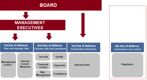
(41) I NTRODUCTION ”There are no accidents; there is only some purpose that we haven’t yet understood.” (Deepak Chopra). The objective of the present Part I is to provide a brief overview of the Risk and Capital Management of financial institutions with the aim to present and explain how leading banks use quantitative models in their daily operations for capital planning and budgeting, measuring and managing risks, stress testing, pricing derivatives or loans and to emphasize their underlying nature based on measure theory. Furthermore, we point out and discuss some potential sources of model risk associated with the use of these models arising in any stage of the model development and deployment process, i.e. from original conception to final use. Although the focus of this Part I is on models used for risk and capital management, many of the issues discussed here apply to models used for other business purposes as well.. Managing risk and capital are at the core of financial institutions activities and fundamental to their long– term profitability and stability. Risk and capital management is not only required by regulators, 6 e.g. see [9], [49], but having an effective risk and capital management in place is fundamental to the business activities of leading financial institutions as it represents an integral part of the long–term strategic and business planning process. Risk is a measure of adverse deviation from the expectation, expressed at a level of uncertainty (probability), while capital is the value of the net assets of the owners of an institution with the primary purpose, from a bank perspective, to absorb risk. In such a way, taking risk is closely related to business activities, development, and customer needs, 7 and it directly depends upon the ability of an institution to evaluate, manage and price risks while maintaining adequate capital and liquidity to meet unforeseen events. Risk and capital are managed via a framework of principles, organizational structures, measurement and monitoring processes that are closely aligned with the activities of the divisions and business units. Capital is managed using regulatory and economic capital metrics, at both business line and legal entity level. Risks are controlled at individual exposure levels as well as in aggregate within and across all business lines, legal entities and risk types. By understanding what risk means, the spectrum of different attitudes towards risk, and a basic process framework for managing risk, institutions can not only mitigate unwanted risks but turn challenges to opportunities. Although financial institutions place varying emphasis on different aspects of risk governance, there is a common theme to employ the role of the three lines of defence governance model, as developed by the Institute 6 The ICAAP within the Pillar 2 of the Basel framework [9] requires credit institutions to have in place an internal risk and capital management. which is adapted to institution specific risk profile; to establish procedures to calculate and safeguard their risk–bearing capacity and to manage their risks. 7 Risk has traditionally been viewed as something to be minimized or avoided, with significant effort spent on protecting value. However, risk is also a creator of value and, approached in the right way, can play a unique role in driving business performance.. 31.

(42) of Internal Auditors in 2013 [61]. The objective of this model is to provide a framework for managing enterprise risk at the strategic, tactical and operational levels and to set out how risks can be manage effectively. The model distinguishes between functions that own and manage risks, functions overseeing risks and functions providing independent assurance. It is used to manage uncertainty and mitigate downside risk, and it enhances understanding of risk management and control. The responsibilities of each of the three lines are: 1. The first line — front line management: directly responsible for identifying and managing risks, i.e. risk owners, developers and users. Their responsibilities are defining, developing, implementing, and operating the model, monitoring its performance and managing changes. 2. The second line — risk management and compliance functions: considers the management of implementation, which involves oversight and effective execution of the risk management framework by the various senior risk management and compliance committees. This line is responsible for establishing policies and standards, performing model risk assessment, managing and inventory of models, independent monitoring of model performance, model usage, and adherence to management policies, reporting to board/senior management. 3. The third line — internal audit and other independent assurance providers: this line of defence has an assurance function that remains independent and objective, and so provides an independent assessment of the adherence of the first and second line of defence to risk policies. They operate in coordination with one another in order to maximize their efficiency and strengthen their effectiveness.. All three lines of defence should be independent of each another and accountable for maintaining structures that ensure adherence to the design principles at all levels. In addition, the Financial Stability Institute (FSI) [13] suggests to consider also a fourth line representing the external audit and supervisors.. Figure 3: The structure of the four lines of defence model as proposed by FSI.. 32.