Chemically Dissected Rotation Curves of the Galactic Bulge from Main sequence Proper Motions
53
0
0
Texto completo
(2) The Astrophysical Journal, 858:46 (53pp), 2018 May 1. Clarkson et al.. Baade’s window, allowing the first test of bulge chemical and kinematic codependence using proper motions. No statistically significant discrepancy in proper-motion dispersion was found between metal-poor (defined as [Fe/H]<0.0) and metal-rich ([Fe/H]>0.0) objects (with Galactic latitudinal proper-motion dispersion difference Δσμ,l≈0.5±0.6 mas yr−1 between the samples), although the sample size was not large. Zhao et al. (1994) combined the Spaenhauer et al. (1992) ground-based proper motions with published radial velocities and metallicities to demonstrate a break in vertex deviation near [Fe/H]∼−0.5. Soto et al. (2007, 2012) demonstrated consistent variation of vertex deviation using Hubble Space Telescope (HST)proper motions for bright giants (for which spectroscopic abundances and radial velocities completed the set of observational parameters; Babusiaux (2016) shows a more recent compilation of vertex deviation as a function of metallicity). The implications of observational chemical-dynamical correlations for formation models of the inner Milky Way are the subject of vigorous ongoing observational and theoretical research. For example, Debattista et al. (2017) showed that samples drawn from a continuous metallicity distribution in a pure-disk galaxy model can be “kinematically fractionated” by bar formation into metal-rich and metal-poor populations with quite different morphology and dynamics, depending on their initial (galactocentric) radial velocity dispersions. (In this scenario, radial velocity dispersion and metallicity each correlate with the time at which the population formed; thus, they correlate with each other.) This is consistent with the tendency of the “X” shape to be preferentially populated by metal-rich stars (e.g., Vásquez et al. 2013, although the magnitude of this preference is somewhat uncertain; see, e.g., Nataf et al. 2014). Bias in the “X” shape toward metal-rich stars has now also been observed in NGC 4710, a nearby diskdominated galaxy viewed almost edge-on (Gonzalez et al. 2016, 2017). Shen et al. (2010) argue that the radial velocities and morphology of bulge stellar populations show no need for a substantial spheroidal “classical” bulge component (at the level of 8% of the disk mass), arguing that the Milky Way can be characterized as a pure-disk galaxy. Nonetheless, a small spheroidal component probably has been detected, although its likely contribution to the total bulge mass is likely well under 10% (Kunder et al. 2016). Interpretation of this component in the context of Galactic formation is not clear; it might, for example, represent part of the halo population that has also probably been detected in the inner Milky Way (Koch et al. 2016).. from the inner halo) showed no strong evidence for a rotational trend. More recently, Kunder et al. (2016) found that their metal-poor RR Lyrae sample with mostly subsolar metallicities (−2.4<[Fe/H]+0.3, peaking at [Fe/H]∼−1.0) shows no strong signature of rotation from radial velocities in any Galactic latitude range. This is in contrast to the majority-bulge population, which shows bulk rotation with amplitude vGC±≈80 km s−1progressing from the first to fourth Galactic quadrant (e.g., Howard et al. 2009; Kunder et al. 2016). This rotation-free component is estimated to be a rather small part of the overall bulge stellar population (Kunder et al. 2016). Restricting attention to [Fe/H]−1.0 (to sample mainly bulge and disk stars), the body of more recent spectroscopic studies does not show strong evidence for metallicity dependence of radial velocity rotation curves (usually plotted against Galactic longitude). For example, the ARGOS survey (Ness et al. 2013b) and the Gaia-ESO survey (Williams et al. 2016) each show no strong difference between metalrich and metal-poor bulge objects (the studies use slightly different cuts for metal-rich and metal-poor objects). However, the Giraffe Inner-Bulge Survey (GIBS, which is unusual among the spectroscopic studies in reaching as close as b=−2° to the Galactic midplane) shows a possible difference in rotation curve slope between objects at [Fe H] < -0.3 and [Fe/H]>+0.2; however, at about 1.5σsignificance, the difference is not yet compelling (Zoccali et al. 2017). Thus, the radial velocity surveys focusing on the majority-bulge population (with [Fe/H]−1.0) show no strong metallicity dependence in the trends of mean radial velocity against Galactic longitude. Proper motions offer an independent method to kinematically chart the bulge rotation curves and, if information on chemical composition is available, explore whether multiple abundance samples really do show distinct mean motions, as well as the well-established velocity dispersion differences. To date, proper-motion investigations in the context of multiple populations (or a continuum) have mostly been performed using bright giants. For example, in addition to the vertex deviation investigations reported in the previous section, proper motions of bulge giants using OGLE (Poleski et al. 2013)and with the Wide Field Imager on the La Silla 2.2 m telescope (Vásquez et al. 2013) have been used to uncover azimuthal streaming in the bulge X-shaped structure. However, Qin et al. (2015) caution via N-body models that the underlying bar pattern speed cannot directly be constrained just from the near-side/far-side longitudinal proper-motion difference. The above radial velocity and proper-motion studies all use bright giants as tracers, often red clump giants (RCGs), which are much less spatially crowded from the ground than are mainsequence (MS) objects. This causes them to be limited by the small intrinsic population size per field of view. For example, ARGOS typically observed about 600 stars at [Fe/H]>−1.0 per 2◦-diameter field of view (Ness et al. 2013b). Thus, mean velocities interpreted for rotation trends represent averages both over quite large angular regions on the sky and, more importantly, over the entire distance range along the line of sight. To make further progress, an independent measure of bulge rotation is needed, using a tracer sample sufficiently populous that the sample can be dissected by line-of-sight distance to mitigate the statistical limitations of giant branch tracers. MS. 1.1. Does Bulge Rotation Depend on Metallicity? In addition to velocity dispersion trends, the trend in bulge mean radial velocity (against Galactic longitude or galactocentric radius) might also be expected to vary with metallicity, but here the magnitude (or even existence) of such a dependence is less clear. Earlier spectroscopic surveys suggest a clear difference between metal-poor and metal-rich samples. For example, Harding & Morrison (1993) and Minniti (1996) demonstrated that “metal-rich” stars show a gradient in circular speed with galactocentric radius, consistent with the “solid-body”-type rotation traced by planetary nebulae (Kinman et al. 1988), Mira variables (Menzies 1990), and SiO masers (Nakada et al. 1993). In contrast, metal-poor objects (using [Fe/H]−1.0, and thus likely including a large contribution 2.
(3) The Astrophysical Journal, 858:46 (53pp), 2018 May 1. Clarkson et al.. velocity ellipsoid. As they point out, detection of Cl,b (or equivalently the orientation angle flb of the proper-motion ellipsoid) allows constraints to be placed on the orbit families for bulge populations, although the conversion from observation to physical constraint is not simple (e.g., Zhao et al. 1994; Häfner et al. 2000; Rattenbury et al. 2007). Clarkson et al. (2008, hereafter Cl08) extended the rotation curve approach, using a much deeper data set with ACS/ WFCtoward the Sagittarius window, estimating photometric parallax directly with reference to a fiducial isochrone describing the average population in the CMD. Consistent with Kuijken & Rich (2002)and Kozłowski et al. (2006), this showed a clear sense of rotation in Galactic longitude, a clear detection of the latitudinal proper-motion trend from near side to far side, and a pronounced peak in the velocity dispersion of both coordinates (σl and σb) coincident with the most densely populated section of the photometric distance range of the sample. Cl08 converted proper motions to velocities, charting the run of the mean velocity (i.e., the rotation curves), the semiminor and semimajor axis lengths (i.e., the velocity dispersions), and the variation of the orientation flb of the projected velocty ellipse with line-of-sight distance, and verified through simulation and comparison with the behavior of RCGs that indeed distance effects are observable in MS photometric parallax (though unlike RCG tracers, unresolved binaries blur somewhat the inferred distances for a given MS population). More recently, in a careful study of three off-axis bulge fields using WFPC2for early-epoch observations and ACS/ WFCfor the late epoch, Soto et al. (2014) were able to extract the rotation curve (and associated proper-motion dispersion curves) for a field farther from the midplane, at (l, b)= (+3°. 58, −7°. 17).12 Soto et al. (2014) also computed the run of velocity ellipse orientation flb with photometric distance, finding trends consistent with Cl08. The kinematics of MS objects at some distance from the plane were thus established to be broadly similar to those at the more central Baade and Sagittarius window fields. Ground-based surveys are now starting to measure proper motions for MS bulge objects. For example, proper motions from the VVV survey have already been used to draw propermotion rotation curves for both giant branch and upper MS populations (although the upper MS population shows much higher proper-motion scatter and substantially different selection effects compared to the giants; Smith et al. 2018). The lack of metallicity information for MS populations has limited both the measurement accuracy and scientific applicability of MS proper-motion rotation curves. The [Fe/H] spread for bulge populations contributes a scatter of up to ∼1mag on the MS (e.g., Haywood et al. 2016), competing with the photometric parallax signal due to the intrinsic distance distribution along the line of sight. While comparison with the behavior of RCGs suggests that indeed the rotation curve can be recovered, a lack of [Fe/H]information for the MS tracers contributes to substantial mixing in photometric parallax that can dilute the signature of underlying rotation (Clarkson et al. 2008). Conversely, charting bulge proper-motion rotation curves from samples partitioned by relative metallicity allows an independent probe of the chemical and dynamical. tracers are orders of magnitude more common on the sky, affording the opportunity to dissect a single sight line along the line of sight, thus offering a “pencil-beam” complement to the wide-field surveys that use the bright end of the CMD.9 It is the charting of the chemically dissected bulge rotation curve from MS proper motions that we report here. Because this is a relatively new technique, we briefly review the short literature in MS proper-motion bulge rotation curve determination before proceeding further. 1.2. Proper Motions of Main-sequence Bulge Populations Proper-motion-based rotation curves10 from MS bulge stars are relatively rare in the literature.11 Kuijken & Rich (2002) were the first to demonstrate the approach for MS populations, for both the Baade and Sagittarius windows, presenting the HST/WFPC2-derived rotation and dispersion curves against photometric parallax (with photometric parallax determined as a linear combination of color and magnitude in order to remove the color–magnitude slope of the MS tracer population of interest). This demonstrated a clear sense of rotation, with the near side of the bulge showing positive mean longitudinal proper motion relative to the far side (a determination made before the much brighter RCGs were used to show bulge rotation from proper motions; Sumi et al. 2004). The propermotion dispersion showed a slight increase in the most populous middle bins of photometric parallax (most strongly pronounced in the latitudinal proper-motion dispersion σb) for their Sagittarius window field. Kuijken (2004) presented an extension of this work to multiple fields across the bulge, including the use of three minor-axis fields to estimate the vertical gravitational acceleration along the Galactic minor axis. Kozłowski et al. (2006)were able to demonstrate similar behavior to the Kuijken & Rich (2002)rotation curves in their analysis of proper motions in Baade’s window. This was the only field for which a sufficiently large sample of sufficiently precisely measured MS stars could be measured from their large 35-field study (which used WFPC2 for early-epoch observations and ACS/HRC for late-epoch observations). While their dispersion curve is consistent with a flat distribution, the rotation trend in Galactic longitude was clearly observed. Kozłowski et al. (2006) may also have been the first to detect the weak trend in latitudinal proper motion μb due to solar reflex motion (see Vieira et al. 2007, for discussion of this effect, including its detection using sets of ground-based observations of bulge giants over a 21 yr time baseline). In any case, Kozłowski et al. (2006) were the first to detect the propermotion correlation Cl,b at statistical significance from any population (using the RCGs that formed their main target population), using it to constrain the tilt angle of the bulge 9. Indeed, bulge giants are so bright that they can be challenging to precisely and efficiently measure from space. 10 Throughout, the rotation curve is defined as the run of the mean proper motion (or transverse velocity) against relative photometric parallax(or distance). The run of proper-motion dispersion (or velocity disperson) is referred to as the dispersion curve. The rotation curve is distinct from the circular speed curve(the run of circular speed about the Galactic center against distance from the Galactic center), which requires projection to cylindrical Galactic coordinates and an assumption of the orbit shape. 11 For clarity of presentation, here and throughout we define the “near side” of the bulge to be the sample closer to the observer than the bulge midpoint along the line of sight, and the “far side” to be its counterpart farther than this midpoint. MS stars on the bulge near side can thus generally be distinguished from their counterparts on the far side by photometric parallax.. 12. This was the only field of the three analyzed by Soto et al. (2014) with a sufficient number of well-measured stars to produce the rotation curve from proper motions.. 3.
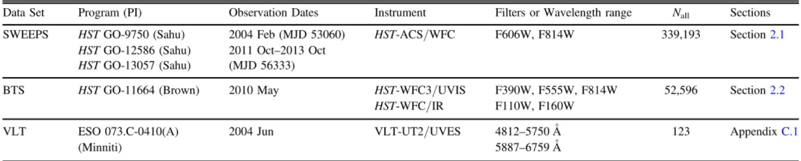
(4) The Astrophysical Journal, 858:46 (53pp), 2018 May 1. Clarkson et al.. Table 1 Provenance of the Observational Data Sets Used in This Work Data Set. Program (PI). Observation Dates. Instrument. Filters or Wavelength range. SWEEPS. HST GO-9750 (Sahu) HST GO-12586 (Sahu) HST GO-13057 (Sahu). 2004 Feb (MJD 53060) 2011 Oct–2013 Oct (MJD 56333). HST-ACS/WFC. F606W, F814W. 339,193. Section 2.1. BTS. HST GO-11664(Brown). 2010 May. HST-WFC3/UVIS HST-WFC/IR. F390W, F555W, F814W F110W, F160W. 52,596. Section 2.2. VLT. ESO 073.C-0410(A) (Minniti). 2004 Jun. VLT-UT2/UVES. 4812–5750 Å 5887–6759 Å. Nall. 123. Sections. Appendix C.1. Note. Nall represents the number of objects in each catalog (with measurements in all filters for SWEEPS and BTS). The median modified Julian dates are indicated for the 2004 and the 2011–2012–2013 SWEEPS epochs. The SWEEPS field lies at (α, δ)J2000.0≈(17:59:00.7, −29:11:59.1), or (l, b)J2000.0≈(+1°. 26, −2°. 65).. correlations resulting from the complex formation and evolutionary processes at work in the inner Milky Way.. This paper is organized as follows. The observational data sets are introduced in Section 2, with the techniques used to classify samples as “metal-poor”or “metal-rich”and to draw rotation curves described in Section 3. The rotation curves themselves are presented in Section 4. Section 5 discusses the implications of our results for the distribution of populations within both the bulge and proper-motion sample selection and discusses the impact of various systematic effects, with conclusions outlined in Section 6. Appendices A–I provide supporting information, including the full set of results in tabular form.. 1.3. Main-sequence Proper Motions for Multiple Populations Until recently, no observational data set existed that would allow the proper-motion-based rotation curves to be charted for multiple spatially overlapping MS metallicity samples in the bulge, as the relevant tracer samples (a few magnitudes beneath the MS turnoff, and well clear of the subgiant and giant branches in the CMD) are far too faint and spatially crowded for objects to be chemically distinguished using current spectroscopic technology. The situation changed with the WFC3 Bulge Treasury Survey (hereafter BTS; Brown et al. 2009), which used threefilter flux ratios to construct a “temperature” index [t ] (a function of F555W, F110W, and F160W magnitudes, similar to V, J, H) and a “metallicity” index [m](using F390W, F555W, and F814W magnitudes, similar to Washington-C, V, I), with scale factors chosen so that [t ]and [m]are relatively insensitive to reddening. This allows stars to be chemically tagged in a relative sense by their location in [m], [t ]space, down to much fainter limits and in regions of higher spatial density than currently allowed by spectroscopy. Brown et al. (2010) showed that indeed the wide bulge metallicity range can be traced photometrically by this method, setting [t ]and [m]indices for tens of thousands of MS objects in each of the four observed bulge fields. Inverting the photometric indices then produced relative [Fe/H]distributions broadly similar to the spectroscopic indications from much brighter objects (e.g., Hill et al. 2011; Johnson et al. 2013). Computing these indices appropriately for objects near the bulge MS turnoff, Brown et al. (2010) found that the candidate exoplanet hosts of the SWEEPS field (Sahu et al. 2006) tend to pile up at the metal-rich end of the [m]distribution as expected, suggesting that [m]is indeed tracking metallicity. Exploitation of this unique data set to directly constrain the star formation history of the bulge is ongoing (see Gennaro et al. 2015, for an example of the techniques involved). Here we combine the relative metallicity estimates from WFC3 BTSphotometry with ultradeep proper motions using ACS/WFC, to construct the proper-motion-based rotation curves of candidate “metal-poor”and “metal-rich” MS samples, and examine whether and how the kinematics of the two samples differ from each other. Our work represents the first extension of chemodynamical studies of the bulge down to the MS.. 2. Observations By the standards of modern proper-motion measurements with HST(e.g., Sahu et al. 2017), the relative streaming motions of the near- and far-side bulge populations are not small, the mean motion of the bulge near side being typically Δμl∼2 mas yr−1relative to the far side, while the foreground disk is separated from the bulge by relative proper motion Dml ~ 4 mas yr−1, although the intrinsic proper-motion dispersion is of roughly similar magnitude (Calamida et al. 2014). Thus, extraction of proper-motion-based rotation curves should in general be reasonably straighforward for many bulge fields for which multiple epochs are available. For this exploratory study, however, we choose the deepest and most precisely measured sample of HSTproper motions available toward the bulge, to minimize complications due to completeness effects and varying measurement uncertainty. This is the SWEEPSdata set, which, with many epochs over a 9 yr time baseline, represents the current state of the art in space-based proper-motion measurement toward the bulge with HST(e.g., Calamida et al. 2015, Kains et al. 2017). We attached SWEEPSproper motions (Section 2.1) to the BTSphotometry (Section 2.2), to afford the maximum sensitivity to proper motions for populations that we can label chemically in a relative sense. Table 1 summarizes the observations. Figure 1 presents a finding chart. The observations cover a single ACS/WFCfield of view (∼3 4×3 4) in the Sagittarius window, a low-reddening region (E (B - V )≈0.5–0.7, depending on the reddening prescription; e.g., Ca15) that is close in projection to the Galactic center (l, b=1°. 26, −2°. 65). 2.1. SWEEPSPhotometry and Proper Motions The SWEEPSdata set used here consists of an extremely deep imaging campaign with a 9 yr time baseline using 4.
(5) The Astrophysical Journal, 858:46 (53pp), 2018 May 1. Clarkson et al.. ACS/WFC pixels) were rotated into a frame aligned with Galactic coordinates and converted from a displacement in pixels into rate of positional change in mas yr−1using the ACS/WFCplate scale (50 mas pixel−1 in the distortion-free frame of Anderson & King 2006)and the time baseline between the two epochs (8.96 yr; Table 1). This yields transverse relative motions in mas yr−1in a frame closely aligned with the Galactic coordinate system. Without absolute reference-frame tracers in this crowded field (e.g., Yelda et al. 2010; Sohn et al. 2012), we work exclusively with relative proper motions. Zero proper motion mf ,0 is defined as the median observed rate of positional change for bulge objects across the entire field of view, without any selection for metallicity. The sample defining this propermotion reference consists of stars that are not saturated in the deep exposures (these objects are at the bulge MS turnoff and fainter).13 Ca15 conducted extensive artificial-star tests to estimate measurement uncertainty in the proper motions, with artificial objects injected with proper motions into individual measurement frames to characterize the random proper-motion uncertainty as a function of apparent magnitude. Including random measurement uncertainty, random intrinsic uncertainty due to tracer star motion, and estimated residual distortion, the proper-motion uncertainty per coordinate is approximately 0.12 mas yr−1over the apparent magnitude range of interest (see Appendix A for details), easily sufficient to measure relative stellar motions in this field. The result is a set of 339,193 objects with ACS/WFC positions, apparent magnitudes, and proper-motion estimates, all with uncertainties characterized as a function of apparent magnitude. Exploitation of these data is presented in Calamida et al. (2014, 2015) and Kains et al. (2017).. Figure 1. Finding chart for the SWEEPSACS/WFCand BTSWFC3data sets used in this work. The tilted solid dark magenta grid shows Galactic coordinates, spaced at 0°. 02intervals. The dotted gray grid shows equatorial coordinates, spaced at 1′intervals. The green polygon shows the BTSWFC3coverage; our sample is drawn from the region of overlap between the two surveys. North is up, east left, and the ACS/WFCfield of view is approximately 3 4×3 4, centered approximately at (α, δ)J2000.0=(17:59:00.7, −29:11:59.1), or (l , b )J2000.0 » (+1 . 26, -2 . 65). See Section 2.. ACS/WFCin F606W and F814W(programs GO-9750, GO-12586, and GO-13057; PI K. C. Sahu). The observations and analysis techniques used to produce the proper motions and photometry used herein are described in some detail in previous papers (Sahu et al. 2006, hereafter Sa06; Cl08; Calamida et al. 2014, hereafter Ca14; Calamida et al. 2015, hereafter Ca15; Kains et al. 2017). Here we briefly describe the relevant characteristics for the present study. Stellar positions in individual images were estimated using the distortion solution and effective point-spread function (PSF) methods developed by J. Anderson for HST and implemented for ACS/WFCin the img2xym.Froutine (Anderson & King 2006) and associated utilities. This yields highly precise position measurements in a reference frame that is nearly free of distortion. With these techniques, per-measurement random uncertainties are as small as X , Y » 0.002 pixels per coordinate (e.g., Figure3 of Cl08), and residual distortion is as low as ∼0.01 pixels (Anderson & King 2006; see also Appendix A). Detailed discussion of the methods can be found in Anderson & King (2006) and Anderson et al. (2008a, 2008b). The 2011–2012–2013 epoch consists of 60 (61) images in F606W(F814W) taken with an approximately 2-week cadence, while the 2004 epoch consists of 254(265) exposures in F606W(F814W) taken over a 1-week interval in 2004 (Sa06, all exposures in both programs being ≈5.5 minutes each, which well samples the bulge MS and minimizes downtime for buffer dumps). Because the disk and bulge stars move relative to each other, the 2011–2012–2013 images were reduced separately from those in the 2004 epoch. Proper motions were derived from the best-fit positional differences between the 2004 and 2011–2012–2013 data sets; they thus represent two-epoch proper motions, but with positions in each individual epoch measured to very high accuracy. The positional differences (in. 2.2. WFC3Photometry from the WFC3 Bulge Treasury Project (BTS) The WFC3 Bulge Treasury Project (BTS; program GO-11664; PI T. M. Brown) visited four fields in the bulge, with WFC3, including the SWEEPSfield. The observations are described in detail in Brown et al. (2010); here we briefly summarize the characteristics relevant for the present paper. In each field, observations were taken in UVIS/F390W (11,180 s), UVIS/F555W (2283 s), UVIS/F814W (2143 s), IR/F110W (1255 s), and IR/F160W (1638 s), with IR images (field of view 123″×136″) dithered in order to fully cover the UVIS observations (field of view 162″×162″). Good overlap was achieved with the SWEEPSACS/WFCobservations; nearly all the BTSobjects in this field also fall within the SWEEPSACS/WFCfield of view (Figure 1). Version 1of the BTScatalog,14 which we use here, employed photometry and positions measured with daophotII (Stetson 1987; Brown et al. 2010). The resulting BTSv1 catalog lists 400,424 objects in the Sagittarius window with reported apparent magnitude in any of the BTSfilters. Of these, 52,596 13. Some notational clarification is in order: although all the proper motions are reported relative to the average motion of a sample defined by the astrometric signal-to-noise ratio, we follow standard practice in this subfield (e.g., Kuijken & Rich 2002) and refer to these relative proper motions simply as “proper motions” m =(ml , mb ), rather than Δm ,to avoid cluttering the notation. 14 A second version of the BTScatalog was released when the present work was at an advanced stage. This second catalog version is discussed in Appendix H: while the measurement techniques are improved over the first version, the differences do not impact the results presented in this work.. 5.
(6) The Astrophysical Journal, 858:46 (53pp), 2018 May 1. Clarkson et al.. Table 2 Vertices of the Selection Polygon in the SWEEPSCMD That Was Used to Select Objects for Further Proper-motion Study (F606W–F814W) (mag). F606W (mag). 1.40 1.54 1.34 1.17. 24.80 21.30 20.50 23.80. Note. See Section 3.2 for discussion.. have measurements in all five of the BTSfilters that are required to construct [t ], [m]estimates. 3. Analysis. Figure 2. Region selection in the SWEEPSCMD. The dashed polygon shows the selection region for objects selected for proper-motion study (see Section 3.2 and Table 2). To illustrate typical stellar parameter ranges for this sample, also overplotted is a 10 Gyr isochrone at [Fe/H]=−0.09 from the “canonical” α-enhanced set within the BaSTIlibrary (Pietrinferni et al. 2004, using the “F05” opacities of Ferguson et al. 2005). The isochrone is plotted twice, color-coded to show log(g)(left color bar) and Teff (right color bar) and offset for clarity, with color minima and maxima set to the range of parameters across the sample of interest. See Sections 3.2 and 3.3.. To construct the “metal-rich”and “metal-poor”rotation curves, we used the BTSphotometry to draw “metal-rich”and “metal-poor”samples by use of [t ], [m]and used the SWEEPS data to estimate the relative photometric parallaxesand proper motions. Within each sample, the relative photometric parallax(p¢) for a given star is defined as the apparent magnitude offset from the fiducial ridgeline in the SWEEPSCMD for the sample. The SWEEPSdeep (F606W, F814W) CMD was used to estimate p¢because this choice of filters is relatively insensitive to metallicity variations when compared to, for example, the (C, V-I)CMD presented in Brown et al. (2010). This section is organized as follows: Section 3.1 describes the merging of the SWEEPSand BTScatalogs, with the sample selection for proper-motion study discussed in Section 3.2 and the calculation of the photometric indices [t ], [m]shown in Section 3.3. These indices require a prescription for extinction, discussed in Section 3.4. The classification into “metal-rich”and “metal-poor”samples is discussed in Section 3.5. The kinematic behavior of the two samples was then measured in two ways; a simple 1D characterization of the longitudinal proper motion ml is indicated in Section 3.6, while a more sophisticated dissection of the velocity ellipse with relative photometric parallaxp¢is shown in Section 3.7.. 47,537objects with proper motions and seven-filter apparent magnitudes, with uncertainty estimates for all quantities. 3.2. Sample Selection for Proper-motion Study Two aspects of the sample selection are worth highlighting. First, the selection region in the (F606W, F814W) CMD was chosen to be well clear of the MS turnoff, subgiant branch, and giant branch, to encompass as many stars as possible with good proper-motion measurements, and finally to capture a region over which the MS for a given population is reasonably free of curvature in the CMD. This selection region is shown in Table 2 and Figure 2. Second, the photometric metallicity and temperature indices include coefficients that amplify measurement uncertainty (particularly F110W and F160W, which appear in the temperature index [t ]). For this reason, objects were only selected for further study for which all apparent magnitude uncertainties in the photometric catalog are smaller than 0.1 mag. The successive selection steps isolating the sample for further study are detailed in Table 3. Of an initial sample of 339,193 SWEEPS objects and 400,424 BTS objects, 9700 (∼2.9%) were retained for further analysis.. 3.1. Merging the ACS/WFCand BTSCatalogs The BTSand SWEEPScatalogs were first cross-matched by equatorial coordinates. Although the absolute pointing of HSTis accurate only to ∼0 1(Gonzaga et al. 2012), with F814Wobservations in both data sets,15 matching of similar objects in both catalogs is straightforward (using F555W and F606W measurements in WFC3 and ACS/WFC, respectively, to refine the matches). For the first round of matching, a kd-tree approach was used to cross-match on the sphere, with a 5-pixel radius used for initial matching. In the second round, pixel positions in the two catalogs were cross-matched and fit using a general linear transformation for objects in the 18 F814W 26 range. While the population of good matches transitions to a background of mismatched objects at a radius of ∼2 pixels and larger, the vast majority of crossmatches were somewhat better, falling within a 1-pixel matching distance. The matching process resulted in a list of. 3.3. Production of [t], [m] for the Proper-motion Sample The photometric indices [t ], [m]take the following form (Brown et al. 2009): [t ] º (V - J ) - a (J - H ) [m ] º (C - V ) - b (V - I ) ,. (1 ). with a º E (F555W - F110W) E (F110W - F160W) and b º E (F390W - F555W) E (F555W - F814W), all of which have a dependence on stellar parameters. The median values of these stellar parameters for the proper-motion sample (Teff ≈ 4800 K and log(g)≈4.6)were estimated from an isochrone chosen to overlap the observed sample (see Figure 2; several. 15. Small differences in effective bandpass of the F814W filter between ACS/WFCand WFC3do not significantly impact the cross-matching.. 6.
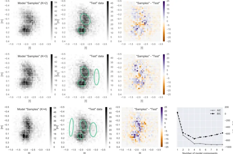
(7) The Astrophysical Journal, 858:46 (53pp), 2018 May 1. Clarkson et al.. combinations of metallicity, age, and extinction were tried, indicating that the parameter range for this sample is roughly 4200 KTeff 5200 K and 4.5 log (g) 4.7).. Table 3 Selection Steps Used to Isolate the Proper-motion Sample for Further Study Selection SWEEPSsample (Calamida et al. 2014) Cross-matched with BTS BTSmeasurements in all filters Within SWEEPSCMD selection region σmag(ACS/WFC)<0.1 mag σmag(WFC3/UVIS)<0.1 mag σmag(WFC3/IR)<0.1 mag Clipping far outliers in [t ], [m]. 3.4. Extinction Estimates for Reddening-free Indices The factors α, βare three-filter extinction ratios (Brown et al. 2009). Synthetic photometry was used to estimate the relationship between reddening and extinctionfor the objects of interest and to generate reddening vectors in the various filter combinations of interest. For a range of E (B - V )values, pysynphot was used to generate synthetic stellar spectra, and the run of AXagainst E (B - V )was fit as AX = kX E (B - V ) separately for all seven filters used in this study, over the range 0.0E (B - V )1.5. The calculation was performed for Teff , log(g)appropriate to the SWEEPS CMD region chosen for proper-motion study (Figure 2). The process was repeated for low- and high-metallicity objects to estimate sensitivity of the extinction prescription to metallicity variation within the sample selected for further study, and for (Teff , log(g)) for objects at the median, minimum, and maximum Teff within this sample to estimate spread of α, β along the sample. This procedure requires a prescription for the extinction law toward the bulge. This extinction law appears to be somewhat nonstandard and strongly spatially variable, with some doubt in the literature about whether a single-parameter model can accurately reproduce observed behavior from the visible to the near-infrared (e.g., Nataf et al. 2016, and references therein). As the [t ], [m]indices use photometry over a very broad wavelength range (CVIJH, or λ≈350–1700 nm), systematic uncertainties in the extinction prescription will in turn impact any inferences about the underlying metallicity distribution (this is one reason why we use [t ], [m] only to classify objects by relative [Fe/H] estimates). To make progress, we adopted a single-parameter reddening law, but with ratio of selective to total extinction RV=2.5, as suggested by the investigations of Nataf et al. (2013).16 As this value is not among the standard parameterizations available in pysynphot, the coefficients AX E (B - V ) for the seven filters were estimated for RV=2.1 and RV=3.1 and linearly interpolated to RV=2.5. Table 4 shows the kXestimates for each filter, along with the coefficients α, β in the [t ], [m]indices. These are quite different from the MS coefficients reported in Brown et al. (2009), as expected since here we are targeting a specific population some way beneath the MS turnoff and have used a different prescription for extinction. For a given choice of RV the variation of all extinctionrelevant quantities appears to be small within the sample of interest; α, β each vary by <0.1 between the two abundance sets tested and, for a given abundance, by 0.02 across the Teff range of this sample. We adopt (a, b ) = (6.44, 1.10) for the rest of this work.. N(remaining). N(removed). 339,193 55,666 47,537 10,225 10,222 10,209 10,145 9,700. L 283,527 8129 37,312 3 13 64 445. Note. The cuts are cumulative, reading from top to bottom. The third step includes selecting out any rows for which any of the seven phometry and two proper-motion measurements are listed as a “bad” value in either the SWEEPSor BTScatalogs. In practice, this limits the sample to 18.5F606W27.5. The SWEEPSCMD selection region is shown in Figure 2. For the three instrumental configurations listed, objects must show photometric uncertainty <0.1 mag in all relevant filters: (F606W, F814W) for ACS/WFC, (F390W, F555W, F814W)for WFC3/UVIS, and (F110W, F160W)for WFC3/IR. Objects passing [t ], [m]clipping satisfy −3.50[t ]−1.00 and −0.60[m]0.40. See Section 3.2 for discussion.. The resulting ([t ], [m]) distribution of objects is shown in Figure 3. Two concentrations are apparent: one near ([t ],. [m])=(−2.0, 0.15), and a second, more elongated concentration with major axis angled at about −45° in Figure 3, centered near ([t ], [m])≈(−2.2, −0.1). To classify objects by relative metallicity and thus draw “metal-rich”and “metal-poor”samples for further study, the population highlighted in Figure 2 was characterized as a Gaussian Mixture Model (GMM) in ([t ], [m]) space, and members of the “metal-poor”and “metal-rich”samples were identified by their formal membership probability Wik (see Appendix B). The number Kof mixture components to use was determined by increasing Kuntil the characterization stopped improving (see Appendix B.2 for details). At least two components seem to be required, but a four-component mixture model appears to provide the best representation of the [t ], [m]distribution. We therefore adopt a four-component GMM to characterize the observed distribution in [t ], [m]space for the rest of this work. Table 5 shows the GMM parameters, while Figure 4 presents the model components visually. The two most significant components correspond roughly to visually apparent concentrations in Figure 3, together accounting for 91%of the mixture; these form our “metal-rich”and “metal-poor”samples. The remaining two components, making up about 6% and 3%, do not correspond to any physically obvious population. These two components might represent populations of outlier objects, or structure in the background in ([t ], [m]). We retain these low-level components in the GMM for all subsequent work using the BTScatalog, but we do not interpret them as representing any intrinsic population component. This four-component GMM provides the basis for our classification of objects by relative metallicity, with “metalrich”and “metal-poor”objects corresponding to the two most significant components of the GMM (Table 5).17. 16. 17. 3.5. Classifying Samples by Relative Metallicity. As a check, the entire kinematic analysis of Sections 3 and 4 was also performed using RV=3.1. Although the mean position of objects in the [t ], [m]diagram shifts slightly when RV=3.1 is adopted, the kinematic trends for the “metal-rich”and “metal-poor”samples are similar to the trends when RV=2.5 is used.. We are not at this stage suggesting that the bulge sample of BTSis intrinsically bimodal in metallicity (as opposed to a continuum of populations; e.g., Gennaro et al. 2015; Debattista et al. 2017). Instead, we are using the photometric indices [t ], [m]to draw samples near the extremes of relative abundance.. 7.
(8) The Astrophysical Journal, 858:46 (53pp), 2018 May 1. Clarkson et al.. Table 4 Estimates of kX º AX E (B - V ) and Derived Parameters CCM89, RV=2.1: log(Z)=−3.3. CCM89, RV=2.1: log(Z)=−1.6. CCM89, RV=3.1: log(Z)=−3.3. CCM89, RV=3.1: log(Z)=−1.6. CCM89, RV=2.5: log(Z)=−3.3. CCM89, RV=2.5: log(Z)=−1.6. ACS/WFC1/F606W ACS/WFC1/F814W WFC3/UVIS1/F390W WFC3/UVIS1/F555W WFC3/UVIS1/F814W WFC3/IR/F110W WFC3/IR/F160W. 1.847 1.064 3.507 2.183 1.074 0.560 0.345. 1.849 1.064 3.492 2.186 1.075 0.558 0.345. 2.786 1.821 4.489 3.167 1.833 1.025 0.635. 2.788 1.822 4.475 3.171 1.834 1.021 0.634. 2.222 1.366 3.899 2.576 1.377 0.746 0.461. 2.224 1.367 3.885 2.58 1.378 0.743 0.460. (F606W–F814W)ACS/WFC1. 0.784. 0.785. 0.965. 0.966. 0.856. 0.857. α β. 7.55 1.19. 7.64 1.18. 5.49 0.99. 5.56 0.98. 6.42 1.10. 6.49 1.09. Config. Note. Here Teff=4800.0 and log(g)=4.59. For convenience, the scale factor for the SWEEPScolor index is also shown. The quantities α, β give the extinction ratios relevant for [t ], [m]. Specifically, a º E (F555W - F110W) E (F110W - F160W) and b º E (F390W - F555W) E (F555W - F814W). See Sections 3.3 and 3.4. Table 5 Parameters of the Gaussian Mixture Model in [t ], [m]Space for Stars beneath the Main Sequence Selected for Further Study k. Name. αk. [t ]0 (mag ). [m]0 (mag). s[2t ][t ] (mag2). s[2m][m] (mag2). s[2t ][m] (mag2). 0. “Metalpoor” “Metalrich” L L. 0.557. −2.18. −0.09. 0.0479. 0.0143. −0.00742. 0.358. −1.97. 0.15. 0.0384. 0.0043. −0.00187. 0.026 0.059. −1.34 −2.87. −0.05 0.01. 0.0153 0.0573. 0.0397 0.0255. 0.00886 0.00240. 1 2 3. Note. Reading left to right, columns indicate the component index k, its label (if any), its (rounded) mixture fraction αk, the two components of its centroid, and the three unique components of the covariance matrix Vk . See Section 3.5.. For an object to be classified with the “metal-rich”or “metalpoor”sample, it must show formal membership probability Wik 0.8 (see Equation (3); note that an object need not be classified with either sample when there are four model components). The shading in Figure 4 visualizes the membership probabilities Wik associated with each mixture component. The threshold Wik 0.8 was chosen as a trade-off between sample purity (typical objects should not fall into more than one model component at the chosen threshold) and the need to have a sufficient sample size (at least a few thousand) to permit the dissection of the proper motions by relative photometric parallaxwith sufficient resolution to chart the rotation curves. Assigning relative photometric parallax(p¢) is the final step required before proper-motion rotation curves can be charted, with reference to fiducial ridgelines for the “metal-rich”and “metal-poor”samples. The fiducial ridgelines themselves were determined by a simple empirical fit to the density of each sample in the SWEEPSCMD. A second-order polynomial adequately represents the median samples and allows very rapid evaluation of relative photometric parallax. Figure 5 shows the adopted fiducial ridgelines for the “metal-rich”and “metal-poor”samples in the SWEEPSCMD, while their parameters are given in Table 6.. Figure 3. [t ], [m]distribution of the population selected for proper-motion study. In the main panel,green points show individual objects, and black contours show the smoothed representation as a 2D kernel density estimate (KDE) with 10 levels plotted. Marginal distributions in [t ]and [m]are shown in the top and right panels, respectively. Typical estimates for measurement uncertainty in this space are presented in Figure 18. See Section 3.3.. A rough estimate for the centroid [Fe/H]values of the two samples may be drawn by charting [Fe/H]contours in the [t ], [m]diagram for synthetic stellar populations and interpolating to estimate [Fe/H]at the [t ], [m]locations of the corresponding GMM component centroids (see Appendix F.1 for more details on the synthetic stellar populations used). The GMM component centroids presented in Table 5 correspond to [Fe/H]0≈+0.18 for the “metal-rich”sample (using scaled-tosolar isochrones) and [Fe H]0 » -0.24 for the “metalpoor”sample (using α-enhanced isochrones for this model component). These centroids are roughly consistent with values suggested from spectroscopic surveys (e.g., Hill et al. 2011; Zoccali et al. 2017). 8.
(9) The Astrophysical Journal, 858:46 (53pp), 2018 May 1. Clarkson et al.. Figure 5. Ridgelines for the “metal-rich”and “metal-poor”samples. The grayscale shows the ACS/WFC (F606W, F814W) Hess diagram for the larger SWEEPSsample. Objects falling within the region of interest for our kinematic study are presented as points, color-coded by “metal-rich”(red) or “metalpoor”(blue). The empirical median-sample ridgelines for the “metalrich”(dark red solid line) and “metal-poor”(blue dashed line) are overlaid. See Section 3.5 and Table 6.. Figure4. [t ], [m]sample color-coded by membership probabilities Wik (Equation (3)) for the k’th model component in the GMM characterization of the observed distribution. The 1σ ellipse for the k’th model component is overplotted in each case as a colored ellipse. Reading clockwise from top left, panels show the “metal-rich,” the “metal-poor,” and the two background components. See the discussion in Section 3.5.. 3.6. Proper-motion Rotation Curves. Table 6 Ridgeline Parameters in the SWEEPSColor–Magnitude Diagram, for the “Metal-poor”and “Metal-rich”Samples. Having drawn “metal-rich”and “metal-poor”samples from the BTSphotometry, along with fiducial sequences in the SWEEPSCMD for the two samples, the “metal-rich”and “metal-poor”rotation curves can be charted. Figure 6 shows the raw distribution of longitudinal proper motion μl and relative photometric parallaxfor the “metal-rich”and “metalpoor”samples, with trends presented in Figure 7. All proper motions in this work were measured relative to the same proper-motion zero-point, defined without reference to any selection by metallicity (Section 2.1). To the extent that the “metal-rich”and “metal-poor”samples trace bulge objects with different spatial distribution and/or kinematic behavior, however, the average proper motions of bulge objects in the two samples might differ. We therefore estimated the proper motion corresponding to the fiducial sequence for each sample. For this “central” proper motion, we used the median proper motion over those sample ¢ and members with relative photometric parallaxbetween Dp¢ magnitudes nearer to and farther than the fiducial, Dp + ¢ =0.05, corresponding roughly respectively.18 We adopted Dp + to ΔD≈0.18 kpcat the distance of the bulge (Section 4.1). The central proper motion for the “metal-rich”sample is then (ml , mb )0MR = (+0.019, +0.19) mas yr−1from 381 surviving objects, while for the “metal-poor”sample we found (ml , mb )0MP = (-0.12, + 0.32) mas yr−1from 290surviving objects. The proper motion corresponding to the “metal-rich” fiducial was thus found to be offset from that of the “metalpoor”fiducial by about (ml , mb )0MR – MP ≈(+0.14, -0.13) mas yr−1.. k. Name. 0 1. “Metal-poor” “Metal-rich”. a0 (mag ). a1. a2 (mag−1). −16.906 −5.720. 48.557 33.458. −14.954 −10.293. Note. These purely empirical ridgelines are used to rapidly evaluate photometric parallax for objects in each sample and take the form F814W = Sj aj x j , with xthe (F606W – F814W) color. See Section 3.5 for discussion.. 3.7. Proper-motion Ellipse Dissected by Relative Photometric Parallax With a difference in rotation curves suggested from the behavior of μl against relative photometric parallax, the next step is to chart the distance variation of the (l, b) proper-motion ellipse. The approach shares several similarities to that reported in Cl08; relative photometric parallaxeswere assigned to each star with reference to the fiducial sequence (appropriate for the metallicity sample with which the star was identified) and the sample partitioned into bins of relative photometric parallaxp¢, with bin widths adjusted so that each bin has the same number of objects. The proper-motion distribution within each bin was fit as a 2D Gaussian, with centroid proper motion m0 and covariance matrix Vm . Uncertainties in fitted quantities were estimated by parametric bootstrapping: synthetic samples for each bin were drawn from the best-fit model, perturbed by the estimated proper-motion uncertainty, and the distribution of recovered parameters over the bootstrap trials was adopted as the estimated parameter uncertainties. Because this process can be sensitive to outliers, a single pass of sigma-clipping was. 18 ¢ was set from the far limit Dp ¢+ using the relation The near limit Dp¢ = 5 log10 (2 - 10 Dp+¢ 5), corresponding to a symmetric selection by Dp distance.. 9.
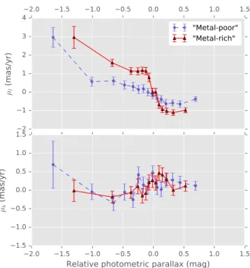
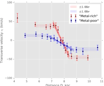
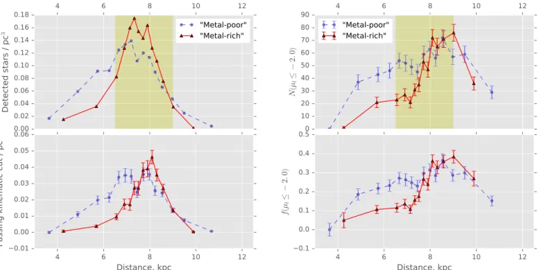
(10) The Astrophysical Journal, 858:46 (53pp), 2018 May 1. Clarkson et al.. Figure 6. Raw distribution of μl against relative photometric parallax(p¢ ), for the “metal-rich”(red) and “metal-poor”(blue) populations. The near side of the population is to the left in both panels. The points themselves are illustrated by colored scatterplots in the main panels, with density contours indicated in gray scale. The top and right panels show the marginal distributions of p¢ and μl, respectively. See Section 3.6.. applied to the proper-motion sample within each distance bin using a ±3σ threshold; this typically removed roughly 1%–2%of the points per bin, with the exeption of the most distant p¢bin (see Tables 16 and 17 in Appendix I). Several improvements were made over the analysis reported in Cl08. For example, rather than subtracting the estimated proper-motion uncertainty in quadrature from the model covariances after fitting, the “extreme-deconvolution” formulation of Bovy et al. (2011)was used, which incorporates estimated measurement uncertainty as part of the fitting process (see Appendix B). We experimented with a multicomponent GMM within each p¢bin for each sample but found a single component adequate (see also Section 5.8). The estimates of proper-motion uncertainty themselves have also been improved compared to Cl08, both in the characterization of random uncertainty through the artificial-star tests of Ca15 and through improved characterization of residual relative distortion (Kains et al. 2017). Details of the adopted uncertainty estimates are presented in Appendix A; for the apparent magnitude range of interest, the total proper-motion uncertainty estimates (i 0.12 mas yr−1)are much smaller than the intrinsic proper-motion dispersion of the bulge (∼3 mas yr−1).. Figure 7. Proper-motion rotation curves. The “metal-rich”sample is denoted in red in the top panel, the “metal-poor”sample in blue in the bottom panel. The population is broken into bins in relative distance modulus and the median value ml determined for each bin (triangles). Faint solid lines show a third-order smoothed spline approximation fit to the binned proper motions ml , while squares indicate equally spaced evaluations of the spline approximation over the range of relative moduli (−1.0(m − m0)<+1.0). See Section 3.6.. 4.1. Distance Conversion and Rotation Curves for the “Metalrich” and “Metal-poor” Samples Figure 11 presents the rotation and dispersion curves of the “metal-rich”and “metal-poor”samples expressed in terms of (D, v ). The conversion of these quantities from the measured (p ¢ , m ) requires the reference distance D0 corresponding to the fiducial sequences for the two samples. The reference distance was set by taking literally the distance modulus (m − M)0=14.45 suggested by studies of the SWEEPS CMD (Ca14), which in turn suggests reference distance (D0 = 7.76 kpc). We assigned this reference distance to both the “metal-rich”and “metal-poor”samples (a choice we examine critically in Section 5.4). Consistent with the simple treatment in Figure 7 and Section 3.6, the “metal-rich”sample shows a higher-amplitude rotation curve than does the “metal-poor”sample, with both a steeper slope and about a factor of ∼2greater difference in mean transverse velocity ávlñbetween the near side and far side of the bulge than for the “metal-poor”sample. To quantify the rotation curve discrepancies between the samples, a simple straight-line model was fit to their rotation curves for distances close to the fiducial for each sequence. This interval was estimated separately for the two samples since their rotation curves appear to level off at different distances from the fiducial (Figure 11). For the “metal-rich” sample the gradient was estimated over the interval D0 0.80 kpc in the (D, vl ) curve (corresponding to −0.24 magp¢+0.21 mag). The rotation curve of the. 4. Results The trends in observed motions are shown graphically in Figures 8–10, while Figure 11 shows the trends after conversion from relative photometric parallaxp¢and proper-motion μto distance Dand velocity v. This information is presented in tabular form in Appendix I. Section 4.1 presents the rotation curves, both observed (i.e., p¢, μ)and after conversion (to D, v), and shows a simple characterization of the trends. Section 4.2 presents the evolution of the velocity ellipse with distance along the line of sight. 10.
(11) The Astrophysical Journal, 858:46 (53pp), 2018 May 1. Clarkson et al.. Figure 8. Variation of proper-motion centroid with relative photometric parallax, for “metal-rich”(red triangles) and “metal-poor”(blue circles) samples, using a binning scheme with 200 objects per bin. The top row shows the proper-motion centroid in Galactic longitude; the bottom row shows the proper-motion centroid in Galactic latitude. Error bars show 1σ uncertainties from parametric bootstrapping, using the best-fit parameters and measurement uncertainties to generate 1000 trial data sets for each distance bin. See Section 4.1.. Figure 9. Semimajor (top) and semiminor (bottom) axis lengths for the propermotion ellipse. Symbols, colors, and error bars as for Figure 8. See Section 4.1.. “metal-poor”sample remains sloped over a broader range, so the fitting interval D0 ±1.4 kpc was used (so −0.44 magp¢+0.36 mag). For both samples the rotation curve amplitude was estimated from the intervals where the rotation curves level off, covering two to three bins each outside the sloped region (Figure 12 indicates the regions used to estimate the rotation curve slopes and amplitudes). The 1σranges of ámlñand ávlñfrom the parametric bootstrap trials were used as estimates of measurement uncertainty in each distance bin, and the trends were fitted to each of the (p¢, ámlñ) and (D, ávlñ) rotation curves separately (rather than transforming the propermotion trends into velocity trends after fitting). We did not attempt to deproject velocities to circular speeds (as discussed in Cl08) but merely attempted to characterize observed trends. Figure 12 and Table 7 show the results. The ratio of the gradients Bwas found to be (BMR BMP )l = 3.70 0.68, while the ratio of amplitudes Ais (AMR AMP )l = 2.29 0.35. Thus, a ratio in rotation curve slopes was detected at approximately 5.4s , while for the velocity amplitude the ratio was detected at roughly 6.5s . The rotation curves in Galactic latitude (Figure 8, bottom panel) visually suggest gentle trends from near side to far side, consistent with previous measurements (e.g., Cl08, Soto et al. 2014). Table 8 reports the straight-line characterization of the Galactic latitude rotation curves, where here we characterized the trend as a straight-line fit within ±2.0 kpc from the fiducial distance D0 . The behaviors of the two samples in μb are statistically similar, with gradient ratio (BMR BMP )b = 0.90 0.87. We do not consider this to represent a secure detection of differing rotation curves in the direction of Galactic longitude.. Figure 10. Variation of the proper-motion ellipse axis ratio (top) and the position angle of its major axis (bottom) as a function of relative photometric parallax. Position angle θ=0° would mean that the proper-motion ellipse major axis aligns with the Galactic longitude axis. Symbols as in Figure 8, with the “metal-poor”sample shown more faintly to avoid cluttering the plots. See Section 4.1.. 4.2. Proper-motion Ellipse Morphology and Amplitudes The velocity dispersion profiles (measured as major- and minor-axis lengths of the proper motion and velocity ellipsoids; Figures 9 and 11) also show differences between the samples. Both samples show a broadly centrally peaked velocity 11.
(12) The Astrophysical Journal, 858:46 (53pp), 2018 May 1. Clarkson et al.. Figure 11. Transverse velocity ellipse centroids (left column) and axis lengths (right column) as a function of estimated line-of-sight distances. Symbols as in Figures 8 and 9, except distance moduli have been converted to line-of-sight distances and proper motions converted to velocities in km s−1. See Section 4.1.. compared to b a » 1.13 0.05; see the top panel of Figure 10). However, the two axis-ratio trends show considerable bin-to-bin scatter. The proper-motion ellipse major-axis position angle also shows trends with relative photometric parallax, although possibly at lower statistical significance than the trends reported in Cl08 despite a much longer time baseline for proper motions (Ca14). This reduced significance may be due to the reduced sample size admitted by the cuts in [t ], [m]employed in this work. It may be that only the “metal-rich”sample substantially shows the proper-motion ellipse tilt with distance, with position angle rising to the 20°–40° range (this tilt is strongly influenced by projection effects; see Section 5.1 and particularly Equation(2) of Cl08). Because the “metal-poor”population tends to be less elongated, its position angle trends are also detected at lower significance. The very nearest relative photometric parallaxbins show behavior consistent with a foreground population dominated by Galactic rotation. This seems particularly clear for the “metalrich”sample, which shows a much more strongly elongated proper-motion ellipse for the nearest bin (a b » 2.0 0.11) and position angle consistent with zero (consistent with differential rotation in Galactic latitude).. Figure 12. Straight-line fits to the inner region of the longitudinal rotation curve along the line of sight, after conversion to velocities and physical distances. The comparison sequences for both samples are assumed to lie at distance D0 = 7.76 kpc . The filled regions indicate ±1.0σ regions for each sample. The horizontal shaded regions show the intervals assumed to be “flat” to estimate the rotation amplitude for each sample. See Section 4.1 and Table 7.. 5. Discussion. dispersion pattern against line-of-sight distance (Figure 11), with the “metal-rich”sample showing a narrower peak, particularly in the major-axis dispersion. The “metal-rich” sample also shows generally lower velocity dispersion by ∼10%, particularly in terms of the velocity ellipse minor axis. Consistent with previous studies (e.g., Soto et al. 2014), the proper-motion ellipse appears to be weakly elongated, with the “metal-rich”population possibly the more elongated of the two samples (with axis ratio b a » 1.29 0.05 at p¢=0. The trends indicated by the union of the BTSand SWEEPSdata sets, particularly the rotation curves (presented in Figures 7, 8, and 11), are quite striking. The “metalrich”rotation curve appears to show systematically greater rotation amplitude than the “metal-poor” sample, shows a greater degree of central concentration along the line of sight (see Figure 11, as well as the raw distributions in Figure 6), and, with the exception of the middle distance bins, may show systematically lower velocity dispersion (Figure 11). 12.
(13) The Astrophysical Journal, 858:46 (53pp), 2018 May 1. Clarkson et al.. Table 7 Trend Parameters for the Inner Bulge Region Gradient(μl) (mas yr−1 mag−1). Amplitude(μl) (mas yr−1). Gradient(vl) (km s−1 kpc−1). Amplitude(vl) (km s−1). “Metal-poor” (MP) “Metal-rich” (MR). −1.78±0.23 −6.85±0.73. 0.48±0.07 1.16±0.07. −18.6±2.66 −68.9±8.04. 18.3±2.58 41.9±2.52. MR–MP MR/MP. −5.07±0.77 3.85±0.64. 0.68±0.10 2.42±0.38. −50.3±8.5 3.70±0.68. 23.6±3.6 2.29±0.35. Sample. Note. See Section 4.1.. produce an apparent rotation curve discrepancy where none were present. Several phenomena might lead the “metal-poor”sample to exhibit greater apparent magnitude scatter than the “metal-rich” sample. First, since the “metal-poor”ridgeline in the SWEEPS CMD is slightly fainter than the “metal-rich”ridgeline, the “metal-poor”objects may be subject to increased photometric uncertainty. Second, at least in principle, if the extinction distribution experienced by the two samples were in some way different, this could lead to a broader apparent magnitude distribution for the “metal-poor”sample. Third, differences in binary fraction between the samples might cause the relative photometric parallax distribution of the two samples to differ, although the nature, magnitude, and direction of such effects may be complex and indeed depend on the class of binaries probed (e.g., Gao et al. 2014). Finally, differences in the intrinsic photometric scatter between the “metal-rich”and “metal-poor”samples might amplify differences between the rotation curves. Our own VLT spectroscopy, as well as spectroscopic campaigns from the literature (e.g., Hill et al. 2011; Zoccali et al. 2017), suggests that the [Fe/H]spread for the “metal-poor”population is greater than for the “metal-rich”population, which would in turn contribute greater p¢scatter in the “metalpoor”population. We have performed simple Monte Carlo tests to determine whether perturbations in the inferred distance distribution can be responsible for the differences in rotation curves between “metal-rich”and “metal-poor”samples. Appendices D and E provide details. In the course of investigating the impact of the differential [Fe/H]distribution on the p¢distribution, it became apparent that the BaSTIset of artificial stellar population methods used to generate synthetic [Fe/H]distributions was (at the time of this work) imposing an apparently artificial population truncation. Appendix F provides details, with the method we adopted to mitigate this selection effect discussed in Appendix E. Perturbations were tested as a result of additional photometric uncertainty or differential extinction variations (Appendix D.1), differences in the fraction of unresolved binaries (Appendix D.2), and differences in the photometric parallax spread caused by differing intrinsic spreads in metallicity (Appendix E). In all scenarios, either the effect is too small to bring the rotation curves into agreement (for binaries), or the required perturbation is too large to have gone unnoticed in previous studies (for extinction), possibly by an order of magnitude (for photometric uncertainty). The strongest single contributor of relative photometric parallaxmixing is intrinsic difference in metallicity spread between the samples;. Table 8 Gradient of Straight-line Fits in Galactic Latitude, for Stars within ±2.0 kpc of the Fiducial Distance D0 = 7.76 kpc Adopted in This Work Sample “Metal-poor” (MP) “Metal-rich” (MR) MR–MP MR/MP. Gradient(μl) (mas yr−1 mag−1). Gradient(vl) (km s−1 kpc−1). 0.26±0.25 0.24±0.28. 4.2±2.76 3.8±2.65. −0.02±0.38 0.92±1.40. −0.4±3.8 0.90±0.87. Note. See Section 4.1.. Before attempting to interpret the trends, however, we examine the magnitude and impact of several potential systematics that might bias the samples, whether by amplifying or even artificially generating the apparent differences in rotation curve (Section 5.1), or by reducing them as a result of mixing in the ([t ], [m]) space used to draw the “metal-rich”and “metal-poor”samples (Section 5.2). The impact of extinction variations along the line of sight, including additional extinction on or past the far side of the bulge, is discussed in Section 5.3. Systematic uncertainties in the final velocity rotation curves due to the proper-motion zero-point and fiducial distance are discussed in Section 5.4. In Section 5.5 we address the question whether the bulge rotation curve from proper motions indeed depends on relative abundance, and we briefly assess trends in proper-motion dispersion in Section 5.6. Implications of the relative photometric parallaxdistributions for the spatial distributions of the “metal-rich”and “metal-poor”samples are discussed in Section 5.7. Because a metal-poor kinematically hot “classical bulge” and/or “halo” bulge component may be present in the inner Milky Way (perhaps more likely among “metal-poor” objects), we attempt in Section 5.8to dissect each of the “metal-rich”and “metal-poor”populations into two propermotion components per sample. Finally, Section 5.9 discusses the implications of our results for the traditional selection of a “clean-bulge” sample using cuts on longitudinal proper motion ml . 5.1. Difference Amplification by Photometric Parallax Mixing Differences in apparent magnitude distribution other than those due to distance spread would contribute to differences in the inferred p¢distributions for the “metal-rich”and “metalpoor”samples. If sufficiently severe, this differential blurring in p¢might cause two intrinsically identical rotation curves to be erroneously measured as discrepant. In the sense of our findings, the “metal-poor”sample might be artificially blurred in p¢compared to the “metal-rich”sample, which would 13.
Figure

+7

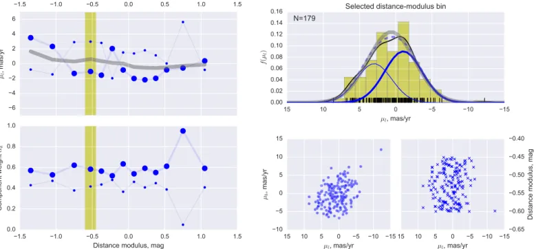

![Figure 19 shows an attempt to reproduce the distribution of [ ]only as a GMM (see Appendixm B for discussion of the technique )](https://thumb-us.123doks.com/thumbv2/123dok_es/7318313.451391/22.918.194.729.84.344/figure-shows-attempt-reproduce-distribution-appendixm-discussion-technique.webp)
Documento similar