CVAR constrained planning of renewable generation with consideration of system inertial response, reserve services and demand participation

Texto completo

(1)PONTIFICIA UNIVERSIDAD CATOLICA DE CHILE ESCUELA DE INGENIERIA. CVAR CONSTRAINED PLANNING OF RENEWABLE GENERATION WITH CONSIDERATION OF SYSTEM INERTIAL RESPONSE, RESERVE SERVICES AND DEMAND PARTICIPATION. ANDRES RICARDO INZUNZA BESIO. Thesis submitted to the Office of Research and Graduate Studies in partial fulfillment of the requirements for the Degree of Master of Science in Engineering. Advisor: HUGH RUDNICK VAN DE WYNGARD. Santiago de Chile, October, 2014.  MMXIV, Andrés Ricardo Inzunza Besio.

(2) PONTIFICIA UNIVERSIDAD CATOLICA DE CHILE ESCUELA DE INGENIERIA. CVAR CONSTRAINED PLANNING OF RENEWABLE GENERATION WITH CONSIDERATION OF SYSTEM INERTIAL RESPONSE, RESERVE SERVICES AND DEMAND PARTICIPATION ANDRES RICARDO INZUNZA BESIO. Members of the Committee: HUGH RUDNICK VAN DE WYNGARD DANIEL OLIVARES QUERO RODRIGO MORENO VIEYRA GONZALO CORTÁZAR SANZ. Thesis submitted to the Office of Research and Graduate Studies in partial fulfillment of the requirements for the Degree of Master of Science in Engineering Santiago de Chile, September, 2014..

(3) To my parents and my brother..

(4) ACKNOWLEDGEMENTS I would like to thank Professor Hugh Rudnick, not only for his devoted work as my professor and supervisor of this thesis, but also for the opportunities and assistance that he has offered me since he accepted me as one of his students. He has been a very important and influential figure in this stage of my life, for which I will be always grateful. I also would like to thank Rodrigo Moreno for his dedicated guidance throughout this whole period. His qualities as a professional and as a person, combined with his incessant curiosity for knowledge have made this journey a truly fulfilling and inspirational one. Additionally, I would like to thank Alejandro Bernales for his valuable assistance during this work. His quick and accurate answers to some of the most crucial questions that arose during this research were of special importance in achieving our goals. Moreover, I want to thank all the people that helped me in the development of this work; Cristobal Sarquis, Daniel Charlin, Felipe Kettlun, Ignacio Urzúa, Ignacio Nuñez, Jaime Larraín, Javier Ayala and Jorge Faundez. I also would like to acknowledge the financial support of CONICYT through the grant Conicyt-PCHA/Magíster Nacional/2013-221320002, Fondecyt 1141082 and Asociación Gremial de Generadoras Eléctricas. Finally, I would like to thank my parents, my brother and the amazing group of friends that have supported me and always been there for me. None of this would ever be possible without your help..

(5) CONTENTS Pag. ACKNOWLEDGEMENTS ........................................................................................ iv CONTENTS ................................................................................................................. v LIST OF TABLES ...................................................................................................... vi LIST OF FIGURES .................................................................................................... vii RESUMEN ................................................................................................................ viii ABSTRACT ................................................................................................................ ix 1.. INTRODUCTION .............................................................................................. 1. 2.. STATE OF THE ART AND CONTRIBUTIONS OF THIS THESIS ............... 3 2.1. Methodological advances of Portfolio Theory applied to the generation sector. ................................................................................................ 3 2.2. Recent applications of Portfolio Theory to the generation sector .............. 5 2.3. Contributions of the present work .............................................................. 7. 3.. METHODOLOGY ............................................................................................. 8 3.1. Nomenclature ............................................................................................. 8 3.1.1. Sets ................................................................................................. 8 3.1.2. Parameters ....................................................................................... 8 3.1.3. Decision Variables ........................................................................ 10 3.2. Optimization Model ................................................................................. 11 3.3. Security of Supply Constraints ................................................................. 16 3.4. Solving Simplifications ............................................................................ 20 3.4.1. Additional Nomenclature ............................................................... 20 3.4.2. Ramping Constraints and Number of Units ................................... 21 3.4.3. Primary Frequency Control Constraints ........................................ 22 3.4.4. Operating Reserve Constraints ...................................................... 26 v.

(6) 4.. RESULTS AND DISCUSSION ....................................................................... 30 4.1. Small-Scale Study .................................................................................... 31 4.1.1. Simulation Set-up .......................................................................... 31 4.1.2. Efficient Frontier of Portfolios ...................................................... 35 4.1.3. Importance of Security of Supply Constraints ............................... 39 4.1.4. Role of Demand Services in the cost-risk Planning Framework ... 44 4.2. Large-Scale Study .................................................................................... 51 4.2.1. Simulation Set-up .......................................................................... 52 4.2.2. Solution Methodology: Benders’ Decomposition Based Algorithm55 4.2.3. Results and Discussion .................................................................. 58. 5.. CONCLUSIONS .............................................................................................. 60. 6.. FUTURE WORK .............................................................................................. 62. REFERENCES ........................................................................................................... 64 APPENDIX ................................................................................................................ 70 A.. SCENARIO MODELING FOR THE LARGE-SCALE STUDY .................... 71 A.1. Fossil Fuel Prices ...................................................................................... 71 A.2. Hydrological Scenarios ............................................................................. 75. B.. DECOMPOSED MODEL’S CONVEXITY PROOF ...................................... 77. vi.

(7) LIST OF TABLES. Pag. Table 4.1: Composition of portfolios shown in figure 4.3 .............................................. 36 Table 4.2: Technically unfeasible frontier portfolios' composition ................................ 40 Table 4.3: Minimum risk portfolio's composition considering different levels of demand response to contingencies ................................................................................................ 47 Table 4.4: Minimum risk portfolio's composition considering different levels of shifted demand ............................................................................................................................ 50 Table 4.5: Technologies input data for the large-scale study.......................................... 52 Table 4.6: Initial and maximum installed capacity of technologies ................................ 53 Table 4.7: Statistic parameters of generated log-normal probability distributions for 2025 fuel prices ............................................................................................................... 54 Table 4.8: Large-scale study’s portfolios composition ................................................... 59 Table A.1: Fuel prices’ returns time series statistical parameters ................................... 74 Table A.2: Base prices and statistic parameters of generated distribution for 2025 fuel prices ............................................................................................................................... 75 Table A.3: Hydrological scenarios characteristics .......................................................... 76. vi.

(8) LIST OF FIGURES. Pag. Figure 4.1: Fuel costs PDFs for the small-scale study .................................................... 32 Figure 4.2: Demand and generation profiles for the small-scale study........................... 33 Figure 4.3: Technically Feasible Portfolios Efficient Frontier ....................................... 35 Figure 4.4: NCRE effect on CVAR of portfolios............................................................ 39 Figure 4.5: Feasible and unfeasible efficient frontiers .................................................... 40 Figure 4.6: Technically feasible frontier and technically unfeasible frontier with security constraints........................................................................................................................ 42 Figure 4.7: Hourly dispatch of the unfeasible minimum risk portfolio .......................... 43 Figure 4.8: Hourly dispatch of the unfeasible minimum risk portfolio operated using all security of supply restrictions (upper bound model)....................................................... 43 Figure 4.9: Hourly dispatch of the unfeasible minimum risk portfolio operated using the lower bound model .......................................................................................................... 43 Figure 4.10: Efficient frontiers considering different levels of demand response to contingencies ................................................................................................................... 46 Figure 4.11: Efficient frontiers considering different percentages of shifted demand .... 49. vii.

(9) RESUMEN La integración de generación renovable puede ayudar a la diversificación de fuentes de energía, mejorando el desempeño económico del sector generación, como también puede significar un incremento en el costo de la electricidad debido a la necesidad de recursos de flexibilidad adicionales que permitan una operación segura, frente al carácter impredecible, variable y asíncrono de este tipo de tecnologías. En este contexto, se propone un modelo de costo-riesgo capaz de planificar la generación y determinar portafolios eficientes, balanceando los beneficios de la diversificación del mix y los costos de mantener la seguridad de suministro incorporando servicios de control de frecuencia y flexibilidad de la demanda, incluyendo la satisfacción de los niveles necesarios de inercia presentes en el sistema. El modelo minimiza el costo esperado de inversión y operación del sistema en base a diversos escenarios hidrológicos y de precios de combustibles fósiles, restringiendo al mismo tiempo la exposición a riesgo de los portafolios a través de su Conditional Value at Risk (CVaR). Problemas de gran tamaño pueden ser resueltos utilizando el modelo (e.g. 8760h y 1000 escenarios) dado que se utiliza programación lineal y se desarrolla un algoritmo basado en descomposición de Benders, adaptado para tratar con restricciones de CVaR en el problema maestro. A través de diversos análisis, incluyendo el principal sistema eléctrico de Chile, se muestra los efectos de las tecnologías renovables en la reducción del riesgo hidrológico y de precios de combustibles fósiles, los efectos de la seguridad de suministro en el costo, riesgo y la inversión en renovables y la importancia de los servicios provistos por la demanda en la limitación de la exposición a riesgo a través de la inversión en energías renovables. Palabras clave: Teoría de portafolios, Portafolios de generación, Respuesta de frecuencia y reservas, Economía de sistemas de potencia, Seguridad de sistemas de potencia. viii.

(10) ABSTRACT Integration of renewable generation can lead to both diversification of energy sources, improving the overall economic performance of the power sector, and significant cost increase due to the need for further resources to provide flexibility and thus secure operation from unpredictable, variable and asynchronous generation. In this context, we propose a cost-risk model that can properly plan generation and determine efficient technology portfolios through balancing the benefits of energy source diversification and cost of security of supply through the provision of various generation frequency control and demand side services, including preservation of system inertia levels. We do so through a scenario-based cost minimization framework where the conditional value at risk (CVaR), associated with costs under extreme scenarios of fossil fuel prices combined with hydrological inflows, is constrained. The model can tackle problems with large data sets (e.g. 8760h and 1000 scenarios) since we use linear programming and propose a Benders-based method adapted to deal with CVaR constraints in the master problem. Through several analyses, including the Chilean main electricity system, we demonstrate the effects of renewables on hedging both fossil fuel and hydrological risks; effects of security of supply on costs, risks and renewable investment; and the importance of demand side services in limiting risk exposure of generation portfolios through encouraging risk mitigating renewable generation investment.. Keywords: Mean-risk electricity generation investment, Generation technologies portfolios, Frequency response and reserves, Power system economics, Power system security. ix.

(11) 1. 1. INTRODUCTION Prior to the deregulation of electricity markets, the supply of electricity rested in governmental institutions, which produced and distributed electricity to households and industry as a centralized monopoly. Thanks to technological advances, efficient sizes of power plants became smaller, reducing economies of scale and opening the door for competition in the generation sector (Kagiannas et al., 2004). Due to this fact, deregulation of the electricity sector took place in the early 1980s, shifting governments and public institutions’ efforts towards a merely regulatory and subsidiary role, through which these agents would drive the development of power systems in a way that is socially desirable. In recent years, this role has taken emphasis on the incorporation of non-conventional renewable generation sources into the grid, mainly because of the increasing awareness of society’s impact on the environment and especially on climate change. The effect of these technologies on the cost of electricity is currently a highly researched topic. Despite the fact that renewables provide an obvious saving to the system derived from less fuel consumption, there is a widespread belief that the inclusion of these technologies may increase the overall cost of electricity, especially in the case of variable, and hard-to-predict renewable generation such as wind or solar power (which are also, the most largely available non-conventional sources in most countries). From a standalone point of view, this notion can be sustained on the fact that investment costs of these technologies tend to be high in terms of dollar-per-generated MWh, because of their relatively low average capacity factor (Galetovic & Muñoz, 2013). On the other hand, from a systemic point of view, operation costs may increase due to the fact that large-scale inclusion of intermittent and unpredictable technologies require larger amounts of reserve and higher flexibility of conventional generation (Pérez-Arriaga & Battle, 2012)..

(12) 2. Interestingly, it has been shown in a number of recent studies that even though renewables may increase expected cost of electricity in the long-term, these technologies might in fact reduce risk of this cost (Awerbuch, 2006; Jansen et al., 2006; Doherty et al. 2006; Delarue et al., 2011). As these technologies are independent from fossil fuel price volatility and can be built on a modular fashion, they become a less risky technology in terms of output and investment costs. The main conclusions of these studies indicate that when the risk variable is added to the generation expansion problem, certain amount of renewables may be economically efficient for some level of risk aversion, while not necessarily being efficient when using a classic least-cost framework for the analysis. Nonetheless, how security restrictions in the operation of the grid can affect the investment decision in the cost-risk context has not been satisfactorily studied in the literature (Delarue et al., 2011). As was stated before, intermittent sources of energy pose a number of challenges to operators. This may increase considerably the costs of a generation portfolio, making it imperative to include these costs in every planning study framework. The first objective of the present study is to correctly incorporate security restrictions for operating generation portfolios containing large amounts of renewables into the cost-risk planning problem. With the development of smart grids and smart metering, the idea that only conventional generators have to sustain system security is seen as extremely conservative. In this context, a variety of Demand Side Management (DSM) techniques (Kupzog & Roesener, 2007) can be employed to increase system flexibility and reduce operation costs driven by renewables. In this context, the second objective of this work is to explore how flexibility resources at the disposal of operators can contribute to the dissipation of the costs of operating large quotas of renewables and how these aspects play a role in the cost-risk planning context. By showing the relevance of including risk and the complexities of the system operation in the planning context, the author hopes that this work stimulates.

(13) 3. developments of new, better and more holistic studies to sustain future energy policies, in order to achieve the correct guidance of the generation sector. 2. STATE OF THE ART AND CONTRIBUTIONS OF THIS THESIS In the following, section 2.1 presents a brief review of the evolution of methodologies for applying Portfolio Theory (PT) to the generation sector, with emphasis on the works that were essential to the present investigation. Next, Section 2.2 summarizes a number of additional recent contributions to the subject, which may be of interest for future research. Finally, section 2.4 refers to the specific contributions of the present study. 2.1. Methodological advances of Portfolio Theory applied to the generation sector. Portfolio Theory developed by Harry Markowitz (Markowitz, 1952) is a useful methodology for constructing portfolios of risky assets in a way that the investor is exposed to the least amount of risk for a certain level of expected return. The most important application of this theory is to determine optimal portfolios of financial assets (Fabozzi et al., 2002) although it can also be used for constructing portfolios of other kinds of assets, as will be detailed ahead. It is important to clarify that PT and other uncertainty managing tools can be applied to the generation sector from a private stand-point. Examples of these are Roques et al. (2008) and Street et al. (2009). The focus of this work on the contrary, is to study the whole system’s exposure to uncertainties, which can be done from a central planner point of view. The conclusions drawn from such an analysis serve as a diagnostic tool for regulators and system planners, so they can assess if current market schemes meet efficiency requirements expected from them. The following literature review is focused on works that use the same approach..

(14) 4. PT was firstly applied to the energy sector by Bar-Lev & Katz (1976), who analyzed fossil fuel acquisitions in the US. A long time after, Humphreys & McClain (1998) made an effort to study how the impacts of energy prices volatility to the economy of the US could be reduced by the usage of PT. It was not until the work of Shimon Awerbuch on 2003 that PT was applied to the generation sector to assess the value of renewables in this context. The methodology employed is detailed in Awerbuch & Berger (2003). The authors use the reciprocal of the levelized cost in kWh/US-cent, which represents the cost effectiveness of each technology or “return”. Risk is measured in % as the standard deviation of the Holding Period Returns1 (HPR) of underlying assets (e.g. fossil fuel prices). Considering natural gas, coal, oil, nuclear and wind technologies, the article concludes that adding wind to the year 2000 EU portfolio and to the projected 2010 portfolio would reduce expected cost and risk. Jansen et al. (2006) propose a number of methodological enhancements to Awerbuch and Berger’s work. In this study, a cost-based approach is proposed, leaving behind Awerbuch’s concept of returns and allowing a rather transparent link between cost and risk. In this case, expected cost is the sum of expected investment, fuel, fixed O&M, variable O&M and environmental impact costs and risk is the standard deviation of the same sum, considering correlations between the different cost components and technologies. Moreover, a methodology by which expert assumptions on the parameters assumed to be uncertain can be transformed into standard deviation is proposed. Thanks to this cost-based approach, this report lays de foundation for the combination of classic planning and operation simulation of power systems and PT. Delarue et al. (2011) is the first work to include operational restrictions in the PT framework. The authors build an hourly dispatch model which decides separately how much capacity should be installed in the objective year and how energy should be deployed, while minimizing cost for a certain level of risk (measured as cost variance). 1. The HPR of a certain non-dividend-paying asset can be calculated as. ..

(15) 5. The main contributions show the importance of ramping constraints when considering intermittent renewables, which impacts greatly on the potentially efficient quantities of these technologies. As will be explained ahead, in the same fashion of Delarue et al. (2011), the present work will focus on showing the importance of including a variety of operative aspects in the PT framework, extending the methodology towards a more realistic and complete planning tool. 2.2. Recent applications of Portfolio Theory to the generation sector Thanks to the theoretical advances made by the authors mentioned in section 2.1, a wide range of applications of PT to the generation sector has been developed. Many of these studies contribute to expand the methodology to different aspects of the planning framework. Van Zon & Fuss (2005) apply PT to the optimization of vintages 2 of different fuel-type-technologies. In this study, a cost-based approach is employed and capacity is distinguished from generated energy, as it is done in Delarue et al. (2011). Huang & Wu (2008) extend this approach, incorporating a duration curve-based model to simulate a 20 years period using a vintage model, which decides the deployment of capacity and energy over technological and fuel price uncertainties. To account for the capability of some technologies to adapt to varying loads, Gotham et al. (2009) develop a methodology on which the load duration curve is divided into different segments characterized by different load factors. The authors show that utilizing different load factors produces more efficient portfolios than the meanvariance approach that does not. Doherty et al. (2006) use net-load duration curves to model wind availability in the PT framework. Also, authors include to some extent system adequacy in the. 2. For example, two coal-fired turbines with different efficiencies and costs would constitute as two different vintages..

(16) 6. portfolio calculation by the usage of the LOLE index. In this study, it is concluded that wind may play a role in least-cost portfolios when considering carbon taxes and in the diversified risk-constrained ones. PT can be also applied to quantify the effects of geographic diversification of wind farms. Rombauts et al. (2011) develop a mean-variance-based model used for studying cross-border transmission capacity constraints’ effect on wind diversification. A different approach to include geographic diversification is proposed by Arnesano et al. (2011). In this work, Awerbuch & Berger (2003) methodology is extended to consider different wind and solar PV geographic locations. Another novel approach to the mean-variance analysis is done by Sunderkötter & Weber (2012), who derive analytical optimality conditions of portfolios. None of the above mentioned studies accurately model operational restrictions of the hourly dispatch. To account for this, Vithayasrichareon & Mcgill (2014) propose a post-processing tool to evaluate the pre-calculated portfolios’ performance under different operation scenarios. Additionally, De Jonghe et al. (2010), although without considering risk, propose a least-cost model to study the impact of these restrictions in long-term system planning. This work also includes some flexibility resources for sustaining high quotas of renewables. In the light of the reviewed literature, it can be concluded that no study has adequately considered operational constraints such as frequency control, spinning and standing reserves or inertia requirements. Additionally, demand services have not been included in the cost-risk planning framework, despite the fact that some flexibility resources were employed in the least-cost planning scheme (De Jonghe et al., 2010). Moreover, the effects of hydrological risk in a hydro-thermal system like the Chilean Central Interconnected System (CIS) have never been studied employing a portfolio theory-based planning tool. Although some studies include hydropower generation (Doherty et al., 2006; Huan & Wu, 2007) they do not model hydrological uncertainty, which is of high relevance in this kind of systems..

(17) 7. 2.3. Contributions of the present work In this work, a static planning generation expansion model that simulates all hours of the objective year is developed. This model decides the amount of installed capacity of every technology considered (Coal-fired, Oil, LNG, Reservoir Hydropower, Run-of-the-river Hydropower, Onshore Wind and Solar PV) and the hourly dispatch of energy, while minimizing cost, subject to an upper bound of risk, measured using CVAR of cost. For this purpose, a set of hydrological and fossil fuel prices scenarios is used (scenario-modeled parameters can be extended without changing the structure of the model). The novel contributions of the work are listed next: Inertial response and primary frequency constraints included in the planning framework: By using the theoretical advances of Chávez et al. (2014), a set of restrictions for the modeling of system inertial response and for constraining its under-contingency frequency nadir is developed, in order to ensure frequency stability at all hours of the simulated year. Spinning and standing reserves included in the cost-risk planning framework: When wind and solar PV are incorporated in the operation of a system, potential forecast errors in the availability of these resources demand the presence of reserve for maintaining system security. This requirement is quantified and included in the optimization of the system’s generating mix. Demand participation’s benefits in portfolios are studied: As was stated before, demand services may add considerable flexibility to the system’s operation. This helps to dissipate additional costs of operating the conventional generation park in the presence of intermittent renewable sources. This is new as the effect of demand flexibility has not been yet studied in the cost-risk planning framework. Inclusion of hydrological risk in the cost-risk analysis: Noting the relevance of hydrological uncertainty in a system with high presence of reservoir and run-of-the-.

(18) 8. river hydropower, the influence of hydrological risk in efficient portfolios is studied in this work. Benders’ decomposition-based algorithm built for solving the problem in reasonable times: As the problem is considerably large (1000 operation scenarios, each with 8760 dispatch hours were simulated) a Benders’ decomposition-based algorithm is proposed for solving a number of scenarios in parallel and shortening simulation times. 3. METHODOLOGY In this chapter, the optimization model for determining efficient portfolios of generation technologies is presented. In section 3.1, the employed nomenclature is shown. Next, in sections 3.2 and 3.3 all restrictions of the optimization model are described. As this set of constraints is non-linear and non-convex, section 3.4 explains how the model is linearized for its solution. 3.1. Nomenclature 3.1.1. Sets (Written in Italic Font) : Set of technologies available for deploying in the objective year. : sub-set containing fast start technologies participating in standing reserves. : sub-set containing technologies that are connected through synchronous machines. : sub-set containing technologies that participate in primary frequency control. : sub-set containing technologies that do not participate in primary frequency control. : Set of dispatch hours in the objective year. : Family of sub-sets indexed by elements in , containing the hours in each day of the objective year. : Set of days in the objective year. : Set of simulation scenarios. 3.1.2. Parameters (Written in Normal Font) : Reference installed capacity of reservoir hydro power in [MW]..

(19) 9. ̅̅̅̅̅̅: Maximum deployable capacity of technology i in [MW]. : Existing capacity of technology i in [MW] : Maximum expected cost of the % highest cost scenarios in [$]. : Demand in hour j in [MWh]. Cost of demand decreasing due to demand shifting in [$/MW]. Cost of demand increasing due to demand shifting in [$/MW]. : Amount of curtailable demand in hour j under scenario s in [MW] for the operating reserve time frame. : Amount of curtailable demand for primary frequency control in hour j under scenario s in [MW]. : Maximum percentage of the demand in any hour that can be shifted to other hours. : Maximum percentage of the demand in any hour that can be increased due to demand shifting. : Nominal frequency of the system in [Hz]. : Technologies governors’ frequency dead band in [Hz]. : Minimum frequency allowed under a contingency of magnitude equal to or smaller than in [Hz]. : Fast start reserve parameter that states what percentage of fast starting capacity will form part of operating reserve. : Fuel cost of technology i in scenario s in [$/MWh]. : Inertia constant of the eventually failed unit in [s]. : Inertia constant of units of technology i in [s]. : Hourly average of water inflow of reservoirs in hour j under scenario s, in [m3/s]. : Annualized investment cost of technology i under scenario s in [$/MW-year] (this includes yearly fixed O&M costs). : Losses of stored water due to evaporation and/or seepage in [m3/s / MM m3]. : Maximum and minimum power output of each unit of technology i in [MW]. : Probability of occurrence of scenario s. : Emergency ramping rate of a unit of technology i in [MW/s]. : Run-of-the-river maximum generation in hour j under scenario s in percentage of Run-of-the-river technology’s installed capacity. Solar maximum generation in hour j in percentage of Solar PV technology’s installed capacity. : Maximum time in which operating reserves must be deployed in [hours]..

(20) 10. ̅: Lower and upper bounds of stored water in reservoirs in millions3 of m3 assuming a certain reference installed capacity of reservoir hydro power plants. : Value of lost load in [$/MWh]. Maximum Wind generation in hour j in percentage of Wind technology’s installed capacity. : CVaR parameter that defines the % highest cost. : Maximum contingency magnitude for which primary reserve and inertia requirements are set, in [MW]. : Electrical power in [MW] generated by the usage of 1 m3/s of water flow. : Hourly maximum ramping rate of technology i in [MW/h]. : Solar forecast error standard deviation of hour j in % of solar installed capacity. : Wind forecast error standard deviation in % of wind installed capacity.. 3.1.3. Decision Variables (Written in Italic Font) : Installed capacity of technology i in [MW]. : Total installation and dispatch costs under scenario s in [$] (this does not include the cost of lost load as it is considered independently). ̃ : Scenario s total cost including the cost of lost load in [$]. : j hour demand decrease, under scenario s due to demand shifting in [MW]. : j hour demand increase, under scenario s due to demand shifting in [MW]. : – CVaR auxiliary variable that represents the right deviation of the cost in scenario s to the variable z in [$]. : Generation of technology i in hour j under scenario s in [MWh]. : Lost load in [MWh]. : Number of units online of technology i. : Headroom in units of technology i, in hour j under scenario s destined for primary reserve in [MW]. : Headroom in units of technology i, in hour j under scenario s destined for spinning reserve in [MW].. 3. 1 million =. as used in Chile..

(21) 11. : Volume of stored water in reservoirs at the end of hour j under scenario s in [MMm3]. : Energy lost through spillage in hour j under scenario s in [MWh]. ̃ at the optimum in [$]. : – CVaR auxiliary variable that will be equal to 3.2. Optimization Model The model determines the installed capacity and hourly energy dispatch on the objective year, by minimizing expected investment and operation costs of a set of fossil fuels prices and hydrological scenarios and constraining risk exposure in terms of CVaR. Total cost in each scenario is given by (3.2.2). This does not include the cost of lost load as this is explicitly considered in the objective function (3.2.1), in which all expected costs are minimized. In the power system planning framework, it is a common assumption to consider the long term electricity demand inelastic, therefore the maximum social welfare is reached when fixed and variable costs of the production of electricity are minimized.. ∑. ∑. ∑. (3.2.1). s.t.:. ∑. ∑. ∑. ∑∑. In order to obtain the different risk level generation portfolios,. (3.2.2). -CVaR. constraints (3.2.3)-(3.2.5) (Rockafellar & Uryasev, 2002) are used. The model uses an arbitrarily high. parameter (. –CVaR upper bound) to obtain the minimum cost. portfolio. Using lower values of the. parameter gives lesser risk-exposed portfolios..

(22) 12. Minimum risk portfolio can be computed by using (3.2.5) as the objective function (Rockafellar & Uryasev, 2002).. ̃. (3.2.3). ∑. ̃. (3.2.4). (3.2.5). ∑. Constraint (3.2.6) ensures that the hourly load is met. This includes demand shifting variables that will be explained in detail further ahead. Also, (3.2.7) is included to limit the generation of technologies in any hour to their installed capacity and (3.2.8) sets upper and lower bounds to this capacity.. (3.2.6). ∑. (3.2.7). ̅̅̅̅̅̅. (3.2.8). As it is done in Delarue, et al. (2011), non-conventional renewable generation technologies are modeled through hourly capacity factor profiles, including run-of-theriver..

(23) 13. Constraints (3.2.9) through (3.2.11) impose these technologies generation profiles. The model only considers one profile for Wind and Solar PV technologies but the formulation can be easily extended to include more. Nonetheless, a variety of run-ofthe-river generation profiles are considered due to the fact that these profiles depend on hydrological scenarios. Also, run-of-the-river reserve provision is constrained according to the availability of the resource. (3.2.9). (3.2.10). (3.2.11). Hydro electrical power plants that may store energy are modeled as one reservoir, considering an average, hourly water inflow (in m3/s) which depends on the hydrological scenario, a constant parameter that accounts for seepage and evaporation losses and the possibility of spillage of water if the upper bound of storage capacity is reached. Also, the generated energy is converted to water flow through the. parameter,. which represents the electrical power generated by 1 m3/s of water flow. Equation (3.2.12)4 includes the aspects mentioned above and represents the hourly balance of the stored water in the reservoir. In this equation, the quotient. represents. the amount of installed capacity of the reservoir technology relative to the basal capacity,. . This is necessary because the inflow, minimum and maximum. capacity parameters are computed using data from a real system, which of course has a certain amount of installed capacity. Thus, it is assumed that as reservoir hydropower is added to the system, inflows and storage capacity grow proportionally. (3.2.13) and (3.2.14) set the lower and upper bounds to the stored water in the reservoir. Additionally, equation (3.2.15) imposes that initial and final stored energy are 4. Unit adjustments have been removed from the equation in order to simplify the expression..

(24) 14. as similar as possible. Both cannot be equal due to the fact that losses would make a 0 hydropower portfolio mathematically unfeasible.. (3.2.12). (3.2.13). ̅. (3.2.14). (3.2.15). For the inclusion of supply security constraints, it is necessary to compute the number of online units of each technology in every hour. This is done using equations (3.2.16)-(3.2.18).. (3.2.16). (3.2.17). (3.2.18).

(25) 15. To account for the limited ramping capabilities of some technologies, constraint (3.2.19) and (3.2.20) limit the difference in output of each one between two consecutive hours. This equation states that in the ramping-up (ramping-down) case, this difference cannot be higher than the ramping capability of the units that are connected during both hours plus the output of units connected (disconnected) to meet the desired final generation level. It is assumed that units are both connected5 and disconnected at their minimum output. If the ramping capability of a technology is sufficiently low in comparison to the change in output due to the connection or disconnection of units alone, these restrictions also act as upper and lower bounds for the total change in the generation. For example, if it is economically optimal to largely increase the number of units from one hour to another, so that the sum of the minimum output of the units being connected is greater than the total ramping rate of the units that were already running, the output may increase at its maximum when these last units ramp-up, but it may also increase if these units ramp down. The first case would be the upper bound for the change in output and the second one would be the lower. When this effect occurs while ramping up (and increasing the number of units), equation (3.2.19) acts as the upper bound, (3.2.20) acts as the lower bound. The opposite occurs while ramping down (and decreasing the number of units).. (3.2.19). (3.2.20). 5. It is also assumed that units connected in certain hour remain at their minimum output level until the next dispatch period which is a conservative assumption..

(26) 16. The model may also shift demand between hours of the same day, which is commonly known as load or demand shifting. Equations (3.2.21)-(3.2.22) set upper bound to the percentage of the hourly load that may be shifted and constraint (3.2.23) ensures that the increments and decrements in the load cancel each other so that the total daily demand remains the same.. (3.2.21). (3.2.22). ∑. (3.2.23). ∑. 3.3. Security of Supply Constraints In Chávez, et al. (2014) a simplified dynamic model of Primary Frequency Response (PFR) is developed to formulate a constraint suitable for an Optimal Power Flow (OPF) framework. In the present work, using similar assumptions, PFR constraints are included in the system planning context. Following the definitions used by Chávez, et al. (2014): “Primary Frequency Response (PFR) will be defined to be adequate if system frequency does not drop below a given limit after any single generation contingency” In this report, reserve held for PFR purposes will be referred to as Primary Reserve. Equation (9) in Chávez, et al. (2014) shows that given the post-contingency inertia of the system. , the magnitude of the contingency. and the governors frequency dead-bands. , the nominal frequency. (assumed to be equal for all governors), the.

(27) 17. minimum system ramp that ensures that the frequency of the system will not fall lower than. is:. (3.3.1). In this case, the post-contingency inertia of the system. is given because the. equation is used in the OPF framework, so this quantity which depends on the dispatch regime, may be assumed as a parameter. By using both Chávez, et al. (2014) and Doherty, et al. (2005) formulations of the swing equation, the following relation can be written:. (3.3.2). Where. is the post-contingency kinetic energy of the system. Therefore,. equation (3.3.1) may be written as follows:. (3.3.3). So, the product of the system ramping rate under contingency and the postcontingency system kinetic energy has to be at least equal to the right expression of equation (3.3.3) in order to ensure that the post-contingency frequency nadir will not be lower than. .. Under the same assumptions made by Chávez, et al. (2014), that is to say, unit’s governors respond to the contingency with a constant but conservative ramp rate and that these units do not reach their maximum output while the power balance between the.

(28) 18. load and generation is not restored6, the following restriction ensures that system frequency adequacy is kept in every dispatch hour by keeping the correct system ramping capability and inertia according to equation (3.3.3).. (. (3.3.4). ) (∑. (. ) (∑. ). ). In this expression,. corresponds to the system’s total ramping rate and. ∑. is equal to the post contingency total kinetic energy in the. ∑. system’s units. The latter is quantified as done in Lee & Baldick (2013). The parameter. was added, so that the effect of demand response to a. contingency may be studied. Responsive load is assumed to be instantaneous and analogous to a decreasing in the magnitude of the contingency. As was done by Chávez, et al. (2014), primary reserve constraints are needed to secure that the units that are considered in the system’s ramp rate, keep the necessary headroom for ramping while the contingency is not cleared.. (3.3.5). ∑. (3.3.6) ∑. Constraint (3.3.5) ensures that there is enough total reserve or headroom to clear the fault and (3.3.6), in the same manner as equation (12) in Chávez, et al. (2014), sets an upper bound to the reserve kept in each technology. This last equation is necessary 6. This is ensured by using additional primary reserve constraints explained later on..

(29) 19. for assuring that primary reserves are deployable in the time that takes all of the ramping units to clear the fault7. It is important to note that in this context, we use the emergency ramping rate parameter parameter. of units, which differs from the common ramping rate. used in equations (3.2.19) and (3.2.20).. Spinning and Standing reserves are also considered in the model. From here on, these types of reserves will be referred to as operating reserves and are considered for two purposes; the first is to restore primary frequency control reserves after they have been deployed and the second is to deal with unforecasted changes in variable renewable generation. Thus, the operating reserve requirement must be a function of the contingency magnitude, the non-conventional renewable generation and its installed capacity. This function will be presented explicitly in section 3.5. ∑. (∑. (3.3.7). ). To account for all reserves described above, constraint (3.3.7) is added to the model. It also includes a demand response parameter to study the effect of responsive loads used in the operating reserve time frame. At this point, two demand response parameters have been defined;. and. . The difference between both is their action time frame, which can be the inertial. 7. The clearing time is equal to ∑. governors’ dead bands (. plus the time that takes frequency to fall lower than the. ). Moreover, as this dead band is assumed to be equal in every governor, all. technologies will start ramping at the same time and will finish to do so after ∑. seconds, due to. equation (3.3.6). This implies that constraint (3.3.6) will be always active, which can be easily demonstrated..

(30) 20. response time frame (seconds) or operating reserve time frame (minutes). The same distinction is done for demand services in the U.K.8. In the same manner as equation (3.3.6), constraint (3.3.8) sets an upper bound on the amount of spinning reserve that may be held in each technology, so it can be dispatched in less than. hours.. (3.3.8). Additionally, reserves must be linked to the headroom of all technologies:. (3.3.9). (3.3.10). 3.4. Solving Simplifications Some of the constraints shown above make the optimization problem non-linear and complex to solve. In this section the simplification used for solving the said model are described. 3.4.1. Additional Nomenclature a) Sets : sub-set that includes technologies that participate in primary frequency control and are qualified as “slow” for having low emergency ramping rate.. 8. National Grid (2014)..

(31) 21. sub-set that includes technologies that participate in primary frequency control and are qualified as “fast” for having high emergency ramping rate. : Set that contains the indexes for discretizing variable domain. : Set that contains the indexes for discretizing variable domain. b) Parameters : Emergency ramp rate of units from technologies of type (slow or fast) in [MW/s]. : Inertia constant of units of any technology in [s]. ̅: Maximum power output of each unit n the model in [MW]. : Percentage of wind generation that will be kept as headroom following the operating reserve criterion for the small-scale study. : Percentage of solar PV generation that will be kept as headroom following the operating reserve criterion for the small-scale study. c) Decision Variables : Auxiliary variable that will be equal to the minimum between the numbers of units of technology i, under scenario s, in hour j and hour j-1 when ramping constraints are active. : Number of slow ramping units that participate in primary frequency control. : Number of fast ramping units that participate in primary frequency control. : Number of synchronous online units that do not participate in primary frequency control. : Operating reserve requirement for hour j under scenario s in the small-scale study. : Operating reserve requirement for hour j under scenario s in the large-scale study. : Auxiliary variable used for modeling the operating reserve requirement in hour j. 3.4.2. Ramping Constraints and Number of Units Constraints (3.2.19) and (3.2.20) can be easily linearized using an auxiliary variable which will take the value of the minimum between the numbers of units of a technology in two consecutive hours, only if the ramping constraint is active in the optimum. These equations are replaced by (3.4.2.1)-(3.4.2.4) in the linear version of the model..

(32) 22. (3.4.2.1). (3.4.2.2). (3.4.2.3). (3.4.2.4). Also, as the simplified model is continuous, restriction (3.2.18) must be removed. Hence, the number of units of each technology ends up being a continuous approximation of the integer result. 3.4.3. Primary Frequency Control Constraints These equations pose a bigger challenge for the linearization of the problem due to the nature of their non-linearity. Equation (3.3.4) is convex, so it may be linearized by using tangent planes. In order to reduce the number of planes and computational resources when solving, technologies participating in PFR are grouped according to their emergency ramping rate: Fast and slow ramping technologies. Technologies within the same group are assumed to have the same emergency ramping parameter. A third group is distinguished, which are technologies that do not participate in PFR but are connected through synchronous machines to the system and add inertia to.

(33) 23. it. For this purpose, inertia parameters of units and their maximum power output are assumed equal to all units. The numbers of units of the three groups are calculated using equations (3.4.3.1)(3.4.3.3) and a linear form of equation (3.4.3.4) replaces constraint (3.3.4) in the model.. ∑. (3.4.3.1). ∑. (3.4.3.2). (3.4.3.3). ∑. (. (3.4.3.4). ). (. (. ). ) ̅. The linear form of restriction (3.4.3.4) is equation (3.4.3.5). Without any loss of generality,. was chosen as the dependent variable during the linearization, so. planes are presented as lower bounds of this variable. Equations (3.4.3.6)-(3.4.3.8) are the position coefficients and partial derivatives that define the planes. ̃. [ ] and ̃. m and h that map the dominium of. [ ] can be any function of the indexes and. variables in a discrete way..

(34) 24. [. ̃. ̃ ̃. [. ̃. ̃. ]. [. [. [ ]. (. ̃ [ ]. ̃. [ ]. ). ̅. ̅. (3.4.3.7) ) ) (̃. (. [. (. [ ]. ) (̃. ]. (. ̃ ̃. [ ]). ̃. (3.4.3.6). ̃. ̃. (3.4.3.5). [ ]). ̃. ). (. ̃. ] (. ] (. (. ]. [. ̃. [ ]. ̃. [ ]. ). ̅. (3.4.3.8). ]. ) ) (̃. [ ]. ̃. [ ]. ). ̅. Other non-linear constraint is equation (3.3.6). This restriction is non-convex, so it has to be treated differently. In this case, upper and lower bounds of the optimal solution are computed. The lower bound of the optimal solution is obtained by removing equation (3.3.6). By doing this, the remaining equations make up a lesser constrained model, which solution portfolios are not technically feasible due to the fact that primary.

(35) 25. reserves are not allocated correctly9 within the installed technologies. This is not important because these solutions serve only as a benchmark for testing how far from the optimal are the technically feasible but sub-optimal solutions that are described next. The upper bound of the optimal solutions is computed by solving a particular case of the model, in which only one technology may participate in PFR. This simplifies equations because when only one technology saves primary reserve, constraints (3.3.5)(3.3.6) end up being a simple linear equality. This is reasonable, because if only one technology participates in primary frequency response, all reserve must be stored in that technology. Let. be the only technology that will be committed to PFR. Then, in the upper. bound model, equation (3.4.3.9) replaces both (3.3.5) and (3.3.6).. (3.4.3.9). In this formulation, equation (3.3.4) must also be linearized as done previously. However, it has to be consistent with the assumption that only technology. is. participating in PFR. Equation (3.4.3.10) represents this particular case and it is included in the upper bound model in its linear form.. (. (3.4.3.10). ). (. ) ̅. 9. Total primary reserves are still held, but if equation (3.3.6) is removed, it cannot be ensured that under contingency state, technologies committed to PFR will increase their output without saturating while clearing the fault. If any unit saturates before the clearance of the fault, the ramping rate of the system decreases from ∑ and equation (3.3.7) is no longer a sufficient restriction for frequency control adequacy..

(36) 26. In conclusion, the linear version of the PFR constraints makes up two models; the lower bound model, in which non-linear equation (3.3.4) is replaced by restrictions (3.4.3.5)-(3.4.3.8) and constraint (3.3.6) is removed. And the upper bound model, in which equation (3.3.4) is replaced by the linear form of (3.4.3.10) and (3.3.5)-(3.3.6) are replaced by (3.4.3.9). For the latter, the model has to be run with each technology committed to PFR individually, so the best bound can be selected. 3.4.4. Operating Reserve Constraints As stated before, the operating reserves security criterion for this study consists in holding reserve for contingency purposes and to protect the system for unforecasted changes in the availability of solar and wind resources. In section 4, where results are presented, two studies will be described. The first one is the small-scale study, on which the main trade-offs between, expected cost, risk, security of supply constraints and demand services are studied. The second one is the large-scale study which serves to demonstrate the scalability of the model and to illustrate the usefulness of the Benders’ decomposition-based algorithm that was developed. A different security criterion was employed for each of these studies. The first one, used for the small-scale case, consists in holding reserve greater than the magnitude of the contingency (so there is enough headroom to replace primary frequency reserves after a contingency) and a certain percentage of wind and solar PV generation. The other criterion, used in the large-scale model, consists in holding reserve for replacing primary frequency control reserves as well, but also to account for statistical errors in variable renewable generation forecasts. Both of them are detailed next. a) Small-Scale Study Operating Reserves Criterion This criterion is represented through the following function:.

(37) 27. (3.4.4.1). To represent this function in a linear way,. is used. This auxiliary variable. will be equal to the maximum between the magnitude of the contingency and the percentage of NCRE generation that must be kept as reserve, when the secondary reserve constraint is active.. ∑. (∑. ). (3.4.4.2). (3.4.4.3). (3.4.4.4). For the small-scale study, (3.3.7) is replaced by equations (3.4.4.2)-(3.4.4.4). b) Large-Scale Study Operating Reserves Criterion For simulations of a large-scale model, a more realistic operating reserve requirement criterion was developed. According to Silva (2010), when uncertainty of renewables’ forecasts is considered for reserve and these forecast errors are assumed non-correlated, normally distributed, with zero mean and a certain standard deviation, the reserve requirement including a N-1 criterion for outages may be quantified as follows:. √. (3.4.4.5).

(38) 28. In this equation, the deterministic criterion for outages is combined with the probabilistic one assumed for variable renewable generation, which requires saving 3 times the total standard deviation of the forecast errors. Standard deviations of forecast errors shown in equation (3.4.4.5) have to be computed using a certain forecast rule. As wind and solar radiation are intrinsically different phenomena, the forecast technique must be selected accordingly. The selection of optimal forecasts techniques is out of the scope of this work, so, simple forecast procedures are assumed for obtaining the parameters needed in simulations. Wind availability has no clear relationship to hours of the day as solar radiation does, so, a persistent 4 hour ahead forecast is employed to compute its forecast error standard deviation. This methodology produces one parameter that represents the uncertainty for all hours of the year. Solar radiation, on the other hand, is forecasted using a day-ahead criterion. 4 typical days of radiation are computed (one for each season) and the standard deviation error is calculated for the 24 hours of the day and for every season. The highest of the 4 values computed for every hour is taken as the conservative estimate. At this point, the reserve requirement for the dispatch hour j in the model would be: (. ). (3.4.4.6). √. In this equation, installed capacities are included because forecasts are made in terms of the capacity factor. The must be restored after a contingency.. term represents the amount of primary reserve that.

(39) 29. It can be argued that the above requirement might be too conservative. This is mainly because if, for example, no wind is forecasted for a certain hour, it would not be reasonable to keep reserve for wind purposes. Due to this fact, the following correction is made: (. ) {. (3.4.4.7). √. In this equation, for hours on which the wind capacity factor of the hourly profile used (which is taken as the forecast) is smaller than the total uncertainty, a deterministic criterion is employed, assuming that in the worst case scenario, all scheduled wind fails to occur. On hours where the wind forecast is sufficiently high, the probabilistic criterion is established. The same logic may be applied for the solar technology. Nonetheless, as an individual standard deviation is computed for every hour, the above correction is not needed for typical zero radiation hours (at night, for example). Still, the correction may be done for cloudy days, where the forecasted radiation could be smaller than the uncertainty. In this work this will be neglected for simplicity purposes, maintaining the conservative character of the requirement. As this requirement is non-linear, a conservative linear approximation is made. This approximation, shown in equation (3.4.4.8), is equal to the original function when or. are equal to zero and it has a similar value. when one of these terms is significantly larger than the other. In any case, the linear function is always greater than the original, so it is a conservative approximation.. √. √. (. ). (3.4.4.8).

(40) 30. √. Finally, taking the assumptions described above, and using the linear form of the absolute value function, the operating reserve constraints used in the large-scale model are:. ∑. (∑. (3.4.4.9). ). (3.4.4.10) {. ( √. (. ). (. √. ). ). (3.4.4.11). (. (3.4.4.12) ). Hence, in the large-scale model, (3.3.7) is replaced by equations (3.4.4.9)(3.4.4.12). 4. RESULTS AND DISCUSSION In the following, the input data and results of simulations done employing the model presented in section 3 are described. Due to the fact that running the model for a large number of scenarios and hours of the objective year is highly time-consuming, firstly, a small-scale study is done for exploring the different trade-offs between expected cost, risk, security of supply.

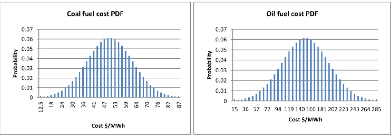
(41) 31. restrictions and demand services and the impact of these aspects in the composition of the generation portfolios. Secondly, a large-scale model, considering 1000 Monte Carlo scenarios of fuel prices and hydrological scenario and the 8760 hours of the objective year is solved using a decomposition algorithm. The main objective of this exercise is to show that the model can be used for solving a realistic planning problem. 4.1. Small-Scale Study This section describes the results obtained from a small-scale study of a generic system. The efficient, technically feasible frontier of generation portfolios is determined and compared to the efficient frontier of unfeasible portfolios, computed using similar operation constraints as done in Delarue, et al. (2011). Also, the way that demand services may dissipate operational costs triggered by the efficient inclusion of renewable generation is studied. 4.1.1. Simulation Set-up In this small version of the model, coal, diesel oil, hydroelectric reservoir, wind and solar PV technologies are included. These technologies will be referred to as Coal, Oil, Dam, Wind and Solar ahead in this document. Also, a second instance of each of the conventional technologies (Coal, Oil and Dam) is considered, so the model may distinguish between conventional technologies that do or do not participate in primary frequency control. These second instances will be referred to as Coalg, Oilg and Damg (“g” stands for governor). These governor equipped technologies are characterized by a 1% higher investment cost (but equal fuel cost) than their non-PFR participants pairs, so the model may decide to install them only if they are needed for PFR purposes. Also, only Oil and Oilg are considered fast-start technologies. Annualized investment costs used are 200 $/kW-year for Coal, Dam and Wind technologies, 50 $/kW-year for Oil technology and 250 $/kW-year for Solar..

(42) 32. Coal and Oil technologies’ fuel costs have an expected value of 50 and 150 $/MWh respectively, and a standard deviation of 12.5 and 45 $/MWh. Also, they are assumed to be perfectly correlated and to have a Gaussian probability function. 40 samples of these distributions are employed for the construction of scenarios and are shown in figure 4.1.. Oil fuel cost PDF. 0.07. 0.07. 0.06. 0.06. 0.05. 0.05. Probability. Probability. Coal fuel cost PDF. 0.04 0.03 0.02 0.01. 0.04 0.03 0.02 0.01. 87. 82. 76. 70. 64. 59. 53. 47. 41. 36. 30. 24. 18. 12.5. 0. 0 15 36 57 77 98 119 140 160 181 202 223 243 264 285 Cost $/MWh. Cost $/MWh. Figure 4.1: Fuel costs PDFs for the small-scale study A 399.67 $/MWh value of lost load is used, according to the short-term failure cost reported by the Chilean regulator10. 3 hydrological scenarios are considered, all of them modeled employing the water inflow parameter (. ) described in section 3.2. All scenarios are characterized. by a constant hourly water inflow, equivalent to a capacity factor of 20%, 40% and 60% respectively. These 3 hydrological scenarios and the 40 samples of both Coal and Oil, perfectly correlated fuel costs make up 120 total scenarios for the small-scale study model. Load, Wind and Solar profiles used are shown in figure 4.2. Average capacity factors of profiles are 28% for Wind and 30% for Solar. 10. Comisión Nacional de Energía (2014)..

(43) 33. One day demand profile Total energy in simulated year: 94.3 TWh. Renewables' generation profiles. 14000. Capacity Factor. 12000. MW. 10000 8000 6000 4000 2000 0 1. 3. 5. 7. 9. 11 13 15 17 19 21 23. 1 0.9 0.8 0.7 0.6 0.5 0.4 0.3 0.2 0.1 0 1. Hours. 3. 5. 7. 9. 11 13 15 17 19 21 23. Wind Profile Solar Profile. Peak: 12.5 GW. Figure 4.2: Demand and generation profiles for the small-scale study As this study’s focus is to measure the benefits from demand services, demand shifting cost parameters are set nearly to zero, 0.0001 $/MW for decreasing any hour’s load and 0.0002 $/MW for increasing it (. and. parameters respectively). This. way, the model decides only to increase or decrease demand, but not both (this saves up results-processing time) and will shift demand whenever optimal. The consideration of cost of demand services is out of the scope of this work, therefore providing an optimistic assessment. Reservoir seepage and evaporation losses are set to 0.5% of stored water in 1 day (this is converted to hourly losses for fitting the model parameters). Also, maximum capacity of the reservoir is set high enough so it does not limit the performance of the Dam technology. Minimum and maximum units’ outputs are assumed to be 50 and 400 MW. Also, contingency magnitude for security constrains is considered equal to a single generator outage (400 MW), the minimum under-contingency frequency allowed is set to 49.2.

(44) 34. Hz11, the nominal frequency value to 50 Hz and governors’ dead-band to. 25 mHz12.. Inertia parameter of all units ( ), including the hypothetically failed one, are set to 5 s. The typical hourly ramp rate parameter ( ) used is 100 MW/h for Coal and 350 MW/h for all other conventional technologies (which is equivalent to an unrestricted ramping rate). Emergency ramping rates ( ), on the other hand, are taken from Chavez & Baldick (2012). Thermal technologies’ ramp rates resulted to be all near to the 10% of their maximum output, in contrast with hydropower technologies that had ramping rates of 2% of their maximum output (in the seconds time-scale, the dynamics governing unit response are different from the hour-to-hour change of output. In this case, thermal units can respond faster than the hydroelectric ones. Kundur, 1994). As was explained in previous sections, in order to save computational resources, technologies were divided into two groups: Fast and slow ramping. After averaging parameters from Chavez & Baldick (2012), emergency ramping rates for Oilg and Coalg technologies (the fast ramping technologies) are set to 38 MW/s and Damg technology’s ramping rate (slow ramping technology) is set to 8 MW/s. Regarding operating reserves, all fast start idle capacity is considered to be part of this reserve ( (. ), and also, 45% of NCRE generation must be held as headroom. 45%). Additionally, it is considered that this reserve must be deployed in 1/3. of an hour or less (. ).. Finally, as explained earlier, all portfolios will be computed using a -CVaR risk measure, with an. 11. value of 95% as done in Street, et al. (2009).. Chilean regulator states that under frequency load shedding must take place when system’s frequency is under the 49.2 Hz threshold. NT/CNE 2009. 12 Maximum allowed governors’ dead-band in Chile. NT/CNE 2009..

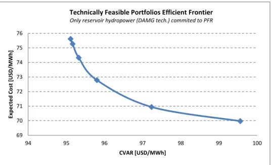
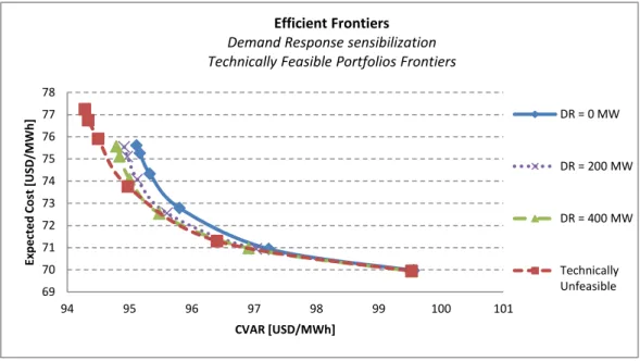
(45) 35. 4.1.2. Efficient Frontier of Portfolios In this section, the efficient frontier for the small-scale model is presented. As was explained in section 3.4.3, in order to solve the model, upper and lower bounds of the optimal solutions were computed. Here, the best upper bound of the optimal is shown (figure 4.3), which is when reservoir hydropower is the only technology committed to Primary Frequency Response. The optimality gap between the lower bound of the solution (which is obtained by excluding equation (3.3.6) from the model and linearizing constraint (3.3.5) through tangent planes) and the upper bound shown in this section, did not exceed 0.6%, hence, feasible sub-optimal portfolios found are highly close to the real optimal frontier. This optimality gap is reduced when demand services are included in the optimization due to the fact that PFR restrictions lose importance when the demand is made more flexible. Therefore, all feasible frontiers shown ahead in this section, present optimality gaps of less than 0.6% in all their portfolios.. Technically Feasible Portfolios Efficient Frontier Only reservoir hydropower (DAMG tech.) commited to PFR. Expected Cost [USD/MWh]. 76 75 74 73 72 71 70 69 94. 95. 96. 97. 98. 99. CVAR [USD/MWh]. Figure 4.3: Technically Feasible Portfolios Efficient Frontier. 100.

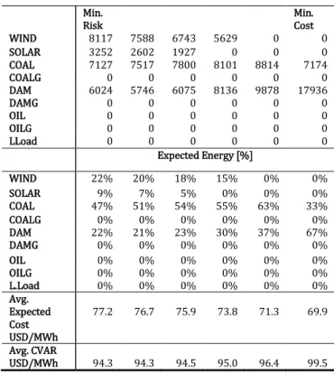
(46) 36. Table 4.1 shows the composition of portfolios in the efficient frontier of figure 4.3. Here, it can be seen that the minimum (expected) cost portfolio contains only hydro-electric capacity and Coal. In this portfolio, a large capacity of hydro-electrical power is installed mainly to maximize the availability of water, which is the best alternative to reduce expected costs. The fact that this could make dry scenarios unnecessarily costly is not relevant when planning with an unrestricted risk criterion. On the other hand, the minimum risk portfolio is formed by a smaller capacity of hydropower, Coal, and both Solar and Wind non-conventional renewables. This result is relevant, in the sense that renewables that under a minimum cost planning framework are not triggered, when the risk variable is included in the optimization, these technologies may appear as economically optimal, even when security of supplies constraints are incorporated. Table 4.1: Composition of portfolios shown in figure 4.3 Portfolios Technology. Installed Capacity [MW] Min. Risk. Min. Cost. WIND SOLAR COAL COALG DAM DAMG OIL OILG LLoad. 5060 2248 8018 0 3925 2534 0 0 0. 5049 1890 8022 0 4353 2533 0 0 0. WIND SOLAR COAL COALG DAM DAMG OIL OILG L.Load. 14% 6% 56% 0% 15% 9% 0% 0% 0%. 13% 5% 56% 0% 17% 8% 0% 0% 0%. 75.6. 75.3. 74.3. 95.1. 95.2. 95.3. Avg. Exp. Cost USD/MWh Avg. CVAR USD/MWh. 4590 2917 1024 0 8171 8537 0 0 5174 6390 2506 2439 0 0 0 0 0 0 Expected Energy [%] 12% 8% 3% 0% 56% 59% 0% 0% 21% 26% 8% 7% 0% 0% 0% 0% 0% 0%. 0 0 8342 0 9664 2475 0 0 0. 0 0 7174 0 16476 1460 0 0 0. 0% 0% 55% 0% 40% 5% 0% 0% 0%. 0% 0% 33% 0% 64% 3% 0% 0% 0%. 72.8. 70.9. 70.0. 95.8. 97.2. 99.6.

(47) 37. Despite the fact that non-conventional renewables are both trigged due to the incorporation of the risk variable, Wind and Solar technologies appear for different reasons. It can be seen in the previous section that Wind technology is cheaper (in $/MWh) than Solar (it has worse capacity factor but the lower investment cost is low enough to make it a cheaper option). Once portfolios’ risk is constrained enough, Wind technology is triggered because in the more expensive scenarios, (high fuel costs and bad hydrological conditions) in relative terms, it becomes a cheap technology. Given these parameters, one should expect that only Wind is triggered. However, the presence of Solar technology can be explained because of its high correlation with the demand profile. When hydropower capacity is reduced, demand peaks become more relevant for fixing the mix. Moreover, as this is only a 1 day simulation, the model is “looking” at a Solar profile that is highly correlated to the load the 365 days of the year, making it an attractive technology when there is low hydropower installed. This was confirmed when a different demand profile (relatively uncorrelated with the Solar profile) was used for simulations. In this case, no Solar capacity was present in the minimum risk portfolio but Wind was still installed. Regarding risk effect on conventional technologies, it is important to note that hydropower capacity is diminished as risk is constrained. This result is in line with the notion that in hydrothermal systems, the first risk factor in costs is the availability of the water resource. On the other hand, Coal capacity is increased as risk is reduced, but when renewable energy is triggered, there is a tendency to lower this capacity. When CVaR is not highly constrained, hydro-electrical capacity is replaced by Coal, as this is a less risky and overall cheap technology. Nonetheless, in high fossil fuels prices scenarios, Wind technology becomes relatively cheaper as Coal fuel costs increase. Hence, when CVaR is constrained sufficiently, Coal is made less attractive due to the fact that.

(48) 38. expensive scenarios become more relevant to define the mix. The consequence of this is that Coal capacity is replaced by Wind. Figure 4.4 illustrates the effect of renewables on portfolio risk. In this graph, a minimum cost portfolio is computed by fixing reservoir hydropower capacity to different levels, CVAR (. ) is then plotted against this capacity. The red curve. shows results by constraining renewable capacity to 0 MW. On the other hand, the blue curve shows the CVAR of portfolios that include the same amount of renewables installed capacity as the minimum risk portfolio of table 4.1. Regarding the non-renewables curve, it was found that as hydropower capacity shrinks, Coal capacity grows and portfolio risk is reduced until a certain level. Once hydropower capacity is small enough, the increase in Coal capacity makes portfolio risk rise again. This exercise is useful to understand that there is not an optimal, single conventional technology when risk is added to the planning framework. Moreover, the curve computed with NCRE in portfolios, show that these technologies may add value to the generation portfolios, as they contribute to achieve lower risk levels if they are added to the mix. In this case, an infinitely risk adverse planner would choose any portfolio containing renewables instead of the pure-conventional ones..

(49) 39. CVAR vs. Hydropower capacity 9000. CVAR [MMUSD]. 8950 8900. CVAR vs. Hydro capacity. 8850 8800 8750. CVAR vs. Hydro capacity With NCRE. 8700 8650 8600 8550 8500 0. 5000. 10000. 15000. 20000. Hydropower Installed Capacity [MW]. Figure 4.4: NCRE effect on CVAR of portfolios. 4.1.3. Importance of Security of Supply Constraints In Delarue, et al. (2011), the authors determine an efficient frontier of generation portfolios using similar restrictions to (3.2.1)-(3.2.23). In that work, the importance of ramping restrictions to account for the limited operational flexibility of a thermal system, which may include variable renewable generation for hedging cost risk, is demonstrated. In this section, as an extension of the cited work, the relevance of security of supply constraints is shown by directly comparing results from a model that includes only ramping constraints and a model that includes both ramping and security of supply restrictions. The efficient frontier obtained by using the model defined only by (3.2.1)(3.2.23) (maintaining the necessary simplifications and linearization explained in section 3.4) will be denominated the “Technically unfeasible frontier” given the fact that security of supply is not enforced in these portfolios. The technically feasible one corresponds to the frontier presented in section 4.1.2..

(50) 40. Figure 4.5 shows both. It can be seen that the technically unfeasible frontier’s portfolios are all in an equal or more efficient region of the risk-cost plane. However, a difference between the portfolios is only notorious for the less risky ones, mainly because when non-conventional renewables are triggered and/or the amount of hydroelectrical capacity is reduced, security of supply restrictions limit the efficiency of feasible portfolios. Efficient Frontiers 78. Expected Cost [USD/MWh]. 77 76 75 74 Technically Unfeasible. 73 72. Technically Feasible. 71 70 69 94. 95. 96. 97. 98. 99. 100. 101. CVAR [USD/MWh]. Figure 4.5: Feasible and unfeasible efficient frontiers In table 4.2 it can be seen that the same tendencies described in section 4.1.2 appear in the unfeasible frontier; as risk is reduced in portfolios, installed capacity of hydropower is also diminished, variable renewables are triggered and Coal capacity increases and then decreases. However, it is important to note that Wind capacity in the minimum cost portfolio is nearly 50% higher than in the feasible frontier. Table 4.2: Technically unfeasible frontier portfolios' composition Portfolios Technology. Installed Capacity [MW].

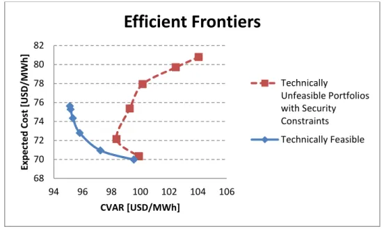
(51) 41. WIND SOLAR COAL COALG DAM DAMG OIL OILG LLoad WIND SOLAR COAL COALG DAM DAMG OIL OILG L.Load Avg. Expected Cost USD/MWh Avg. CVAR USD/MWh. Min. Risk 8117 3252 7127 0 6024 0 0 0 0. Min. Cost 7588 2602 7517 0 5746 0 0 0 0. 22% 9% 47% 0% 22% 0% 0% 0% 0%. 20% 7% 51% 0% 21% 0% 0% 0% 0%. 18% 5% 54% 0% 23% 0% 0% 0% 0%. 15% 0% 55% 0% 30% 0% 0% 0% 0%. 0% 0% 63% 0% 37% 0% 0% 0% 0%. 0% 0% 33% 0% 67% 0% 0% 0% 0%. 77.2. 76.7. 75.9. 73.8. 71.3. 69.9. 94.3. 94.3. 94.5. 95.0. 96.4. 99.5. 6743 5629 0 1927 0 0 7800 8101 8814 0 0 0 6075 8136 9878 0 0 0 0 0 0 0 0 0 0 0 0 Expected Energy [%]. 0 0 7174 0 17936 0 0 0 0. Figure 4.5 must be interpreted carefully. As the unfeasible frontier is computed without security of supply constraints, costs presented in this graph are a sub-estimation of the real costs of operating the installed capacity of each portfolio. The “real” costs and risks of unfeasible portfolios must be computed by operating the installed capacity of portfolios using all security of supply constraints. Figure 4.6 shows costs and risks of the unfeasible portfolios when operated in a secure way. It can be seen that the unfeasible portfolios hid a considerable amount of costs which makes these portfolios much more inefficient than the ones shown in figure 4.5. This result illustrates the necessity of considering a detailed modeling of operation restrictions in the planning framework, which is uncommon in long-term studies. Moreover, in figure 4.6, minimum cost portfolios are highly similar, nonetheless, the difference between the frontiers increases drastically as one moves towards the supposedly less risky portfolios. Hence, it can be said that the relevance of.