On the Prevalence of Supermassive Black Holes over Cosmic Time
10
0
0
Texto completo
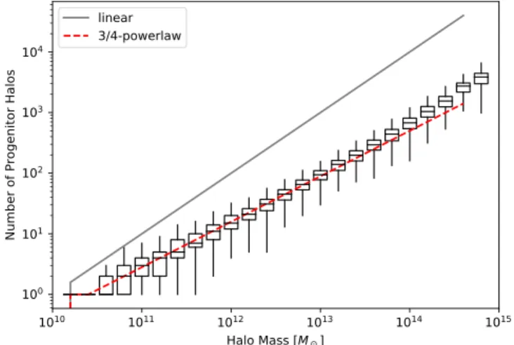
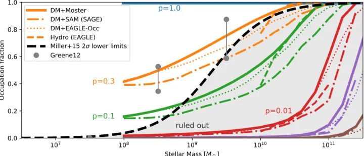
(2) The Astrophysical Journal, 874:117 (10pp), 2019 April 1. Buchner et al.. evolution of the halo and the seeding probability correlate only weakly, this formalism allows for an estimate of the efficiency of the seeding process. We explore the implications of such seeding recipes and viable parameter ranges for Mc and p. Connecting (potentially early) black hole seeding with observations in the local universe requires simulations that follow the mass evolution of the universe. High mass resolution is necessary to follow sites of emerging proto-galaxies. Additionally, because seeds may be rare, large cosmological volumes need to be probed. To this end, we use the MultiDark cosmological dark matter N-body simulations (Prada et al. 2012; Klypin et al. 2016). These assume a Planck cosmology (h=0.6777, ΩΛ=0.693, Ωm=0.307, Planck Collaboration et al. 2014), which we use throughout.5 The simulation evolves an initial dark matter density distribution over cosmic time under gravity. This encompasses the gravity-dominated collapse into sheets, filaments, and finally halos, wherein galaxies should reside, as well as the mergers of structures. To study the evolution of halos, merger trees6 summarize the merging of (sub)halos as well as the dark matter halo mass at each simulation snapshot. In particular we focus on the highestresolution, Small MultiDark simulation (SMDPL) with a box size of 400 Mpc h−1, populated with 38403 dark matter particles of mass 108 Me h−1, which resolves well halos of masses down to 1010 Me. When smaller halo resolution is needed, we use the 40 Mpc h−1 “Following ORbits of Satellites” (FORS; González & Padilla 2016) simulation, whose small particle masses (≈4×10⁶ Me h−1) resolve halos down to 108 Me well. The FORS cosmology is very similar to the abovementioned values. This work adopts virial masses in Meh−1 throughout7 and physical units for all other quantities. Throughout, we refer to the created black holes as seeds or (S)MBHs. However, because we only count the halo occupation, our model does not need to assign any specific mass to them. Our calculations are thus independent of seed mass and mass evolution. Consequently, we refrain from exploring correlations of galaxy properties with black hole mass. Byproducts of the seeding process that do not become MBHs are not considered here, but may additionally be present in the universe.. Figure 1. Number of 1010 Me halos that built a z=0 halo. At each halo mass bin, we count the number of progenitors that merged into each halo. The rectangles with horizontal lines represent the 25%–75% quantile range and median of each mass bin. The vertical line shows the range of the distribution. The red dashed line indicates a 3/4 power-law relation.. power-law relation with subunity normalization: Nz = 0 =. 1 (Mz = 0 Mc)3 2. 4. (1 ). This is plotted as a red dashed curve in Figure 1, and is an appropriate approximation as we will show below. Around this mean number of constituents, Figure 1 shows modest scatter of approximately 0.2 dex. We verified that this relation also holds for other values of Mc (108.5–11 Me). We then compute the black hole occupation fraction. If a halo is made from N building blocks, each with equal chance p to contain a seed black hole, it contains a black hole with probability: P (BH∣N ) = 1 - (1 - p ) N .. (2 ). This is derived by considering the probability that none of the N halos have an MBH, and taking the complement. A subtle point here is that we do not need to keep track of the number of black holes inside a halo and whether/when they merge or get ejected from the system. Equation (2) only assumes that if multiple halos with black holes merge, at least one of these black holes remains in the merged halo. The average of P (BH∣N ) over a halo population yields the expected occupation fraction. Figure 2 plots the occupation fraction as a function of halo mass and seeding fraction p, for the case of Mc=1010 Me. We now constrain p using observations. We focus on a recent measurement of the fraction of local galaxies containing a massive black hole as a function of mass by Miller et al. (2015, M15). They surveyed local early-type galaxies for central X-ray point sources, a telltale sign of accretion onto SMBHs, and carefully corrected for flux limits. Correcting for the X-ray inactive fraction of black holes is systematically uncertain. The correction anchors on the X-ray active fraction at the higher masses, where the occupation fraction is thought to be ∼100% (Greene 2012). M15 used an advanced methodology to incorporate that the X-ray luminosity distribution changes with host mass. They detect sources down to and below host galaxy stellar masses of 109 Me and their inferred lower limits on the black hole occupation fraction are shown in the bottom panel of Figure 3 as a thick black dashed. 3. SMBHs in Local Galaxies Owing to the hierarchical growth of structures, a high number of halos go into building massive galaxies. When halos merge, occupant black holes are generally passed on to the merger product (this assumption is discussed below). This implies that the fraction of halos that need to be seeded could be very low (Menou et al. 2001). As a starting point, we simply count for z=0 halos, from how many 1010 Me halos they were built. Specifically, we count in each merger tree the leaves with M>Mc. This is shown in Figure 1. If galaxies were only built by mergers of existing halos, we would expect a linear relation, Nz=0=Mz=0/Mc (gray line). However, growth through accretion of noncollapsed structures (e.g., filaments) is also important. A better empirical description is a sublinear 5. We explicitly multiply out h, e.g., in distances, but for comparison with the literature we keep halo masses in units of h−1. 6 Constructed with ROCKSTAR and ConsistentTrees (Behroozi et al. 2013a, 2013b). 7 To convert into physical units, our reported masses need to be multiplied by h and divided by ∼0.75 to account for the impact of baryons (see, e.g., Sawala et al. 2013).. 2.
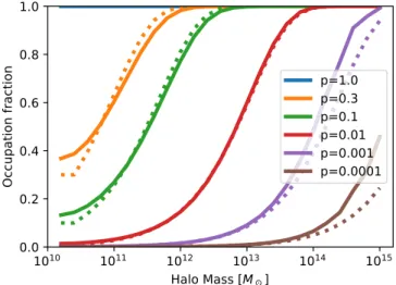
(3) The Astrophysical Journal, 874:117 (10pp), 2019 April 1. Buchner et al.. the constraint: p (Mc 1011M)3 4 .. (3 ). In the following, we consider only models satisfying this constraint. 4. The SMBH Population over Cosmic Time To explore how the SMBH population evolves over cosmic time, we populate the halo tree according to our recipe. When a halo for the first time reaches a mass Mc, with chance p it is marked as occupied by a black hole. The occupation is inherited by the merger tree descendant. As a consequence, in our seeding framework black holes are not only “born” in the high-redshift universe. To show this, the left panel of Figure 5 presents birth rates over cosmic time. Seeding is most frequent at early times (z>4). Depending on the model parameters, the median seeding time lies in the second, third, or forth billion years. At z<6, the model curve shapes are almost independent of the input parameters. Regarding the normalization, we note that a 100% seeding above mass Mc creates a black hole population at a similar rate as 10% seeding at mass 10%×Mc (left panel of Figure 5). As halos containing black holes merge, interactions of multiple SMBHs are possible. The middle panel of Figure 5 shows mergers of halos hosting black holes. The normalization again scales as just described for the birth rate. Changes in the critical mass shift the peak slightly. We explore the possible merging of the black holes themselves in the next section. The right panel of Figure 5 presents the total number of massive black holes over cosmic time. For p=1, this is just the number of halos above the mass threshold. Overall, we find a present-day SMBH space density of >0.01 Mpc−3 (with models not ruled out in Figure 4). In the local universe, the fraction of occupied halos is mass-dependent in the way presented in Figure 3. The comparison between the number of SMBHs to the observed number of AGN provides the fraction of actively accreting black holes in excess of that luminosity threshold. Modern surveys detect hard X-ray emission even in heavily obscured AGN, and recover the intrinsic accretion luminosity using X-ray spectra (e.g., Buchner et al. 2015). In Figure 5 we include the space density of AGN at L(2–10 keV)> 3×1042 erg s−1 and >1044 erg s−1, which correspond approximately to accretion rates of 5×10⁶ and 5×10⁸ Me Gyr−1 (Marconi et al. 2004), respectively, assuming 10% radiative efficiency. The AGN density inferred from observations is 1–3 orders of magnitude below the total SMBH population in Figure 5. The comparison indicates that the vast majority of the SMBH population is dormant or accretes at low levels.. Figure 2. Black hole occupation in the local universe as a function of halo mass. The solid curves are from dark matter simulations. The dotted curves are computed from the analytic Equations (1)and (2). This figure assumes Mc= 1010 Me.. line. Greene (2012) previously reviewed observational constraints and also considered the late-type spiral sample of Desroches & Ho (2009), obtaining slightly elevated lower limits (gray connected points in Figure 3). To compare our simulation to these observational constraints, we convert from halo masses to stellar masses. We test several methods: First, we assign stellar masses from the Moster et al. (2010) conditional stellar mass function P (M∣Mh )8 derived from matching the local stellar mass function and galaxy clustering to simulated dark matter halos. Importantly, this empirical method does not assume any galaxy evolution physics and is observational. Second, we try assigning stellar masses according to the distribution produced by the SAGE semianalytic model for the MDPL2 simulation (Croton et al. 2016) and that produced by the EAGLE hydroradiative simulation. The latter (Schaye et al. 2015, version Recal-L025N0752) reproduces the galaxy mass function and sizes very well, particularly in this mass regime. However, populating halos based only on a Må–Mh distribution neglects that the number of progenitors N could influence Må at a given Mh, inducing a correlation between occupation probability and Må. To test this, we also derive the number of progenitorsN and Må from the merger trees of EAGLE. The groups of curves in Figure 3 demonstrate that for a given p the results from these four methods are consistent. Thus, the choice of the Mh − Må conversion method does not materially affect our conclusions. Figure 3 shows the occupation fraction predictions for Mc=1010 Me. The comparison with the observational lower limit implies p30%, with lower seed probabilities ruled out. For higher masses, even higher seed probabilities are necessary, e.g., Mc=1011 Me matches observations only with full occupation (p=100%). We explore the allowed seeding fractions p by extrapolating Equations (1)and (2) into lower mass regimes. We compute curves like in Figure 3 with the mean Må/Mh ratio of Moster et al. (2010) and accept those that pass the M15 limits. Figure 4 shows the allowed parameter space. Because the number of halo building blocks has a 3/4 power-law exponent (see Figure 1 and Equation (1)), we find. 5. Gravitational Waves from SMBH Mergers The merging of halos in principle brings their SMBHs together as well. The merging of SMBHs produces gravitational waves, detectable with the proposed LISA (Amaro-Seoane et al. 2017). Salcido et al. (2016) predicted in detail waveforms of SMBH mergers from the EAGLE cosmological simulation. Because of the sensitivity down to 104 Me (Amaro-Seoane et al. 2017), Salcido et al. (2016) find that essentially all mergers are within the sensitivity of LISA, with their first mergers of the low-mass SMBH seeds dominating. Therefore, one can neglect mass and sensitivity considerations and focus on the occurance of SMBH merger events. We predict the number and redshifts of observable GW events from our scenarios. In this computation, the rest-frame. 8. We only consider the central galaxies because we work with a subhalo catalog and satellites are unimportant in the mass range of interest.. 3.
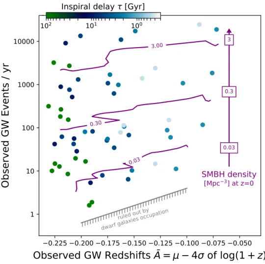
(4) The Astrophysical Journal, 874:117 (10pp), 2019 April 1. Buchner et al.. Figure 3. Black hole occupation in the local universe as a function of stellar mass. Differently colored model curves correspond to different seeding probabilities p. Observational lower limits are shown as a dashed black curve (Miller et al. 2015, 2σ lower limits) and gray connected points (Greene 2012). These imply p30% for the chosen mass limit (Mc=1010 Me). Figure 4 explores other mass limits.. time. These are shown in the inset of Figure 6. These delay functions have the effect of changing the observed merger redshift distribution in a characteristic fashion. For example, the dashed curve in the main panel of Figure 6 is assuming no delay (see also Salcido et al. 2016) between halo merger and black hole merger, while each solid curve applies a different delay function. These generally move the peak to lower redshifts, narrow the distribution, and can suppress the rate of black hole mergers substantially. Overall, all of the distributions appear approximately Gaussian in the scale factor, log a = -log (1 + z ). We define two LISA observables: the number of GW events observable per year, N, and, Ā, which describes the location and shape of the distribution and is defined as: A¯ ≔ m - 4s.. (4 ). The Ā statistic combines the mean μ and standard deviation σ of the log (1 + z ) distribution (see, for example, Figure 6). Through experimentation, we found that an Ā centered on μ but skewed 4σ to the left of the distribution captures well both the shift and narrowing of the redshift distribution caused by merger delays. It can be readily computed from detected gravitational wave events, assuming a cosmology. These two observables diagnose the underlying SMBH population and differentiate delay functions. Figure 7 presents our LISA diagnostic diagram, populated by all combinations of the seeding prescriptions and delay functions. The number of events predicted (y-axis) generally reflects the overall space density of SMBHs (purple contour curves and arrow), and is thus primarily driven by the chosen seeding prescription. It is notable that a wide range of predictions are possible, from few to thousands of events per year. However, even in the most unfavorable scenario with slow inspirals and a high mass threshold (1011 Me), a few detections per year are predicted. The color-coding of the LISA model points in Figure 7 indicates the median delay time corresponding to a delay function in the inset of Figure 6. Because the colors approximately change along the x-axis, the Ā statistic (x-axis) is a proxy for the delay function, and can distinguish slow from quick inspirals (green to light blue. Figure 4. Allowed parameter region (white area) given the M15 limits (see Figure 3). The colored dots are the parameters shown in Figure 3 as thick lines, with the same colors. If seeding is only allowed at z>7, the allowed region shrinks, as indicated by the blue dotted line. Circled numbers allow approximate comparison to some physical seeding models (Volonteri et al. 2003, 2008; Agarwal et al. 2014) and large-scale cosmological simulations (Crain et al. 2015; Schaye et al. 2015; Weinberger et al. 2018).. black hole mergers at a given redshift r(z) within a redshift interval dz in a comoving volume dVc are converted into observable rates dz dV 1 ´ c ´ 1 + z to account for the across the entire sky using dt dz corresponding rest-frame time, comoving volume on the sky and time dilation (e.g., Sesana et al. 2004; Salcido et al. 2016). However, the time delay between halo merger and black hole merger is uncertain. Kelley et al. (2017) explored in detail the physical processes as SMBH binaries overcome nine orders of magnitude in separation from kilo- to microparsecs. They also present several physically reasonable delay functions, quantifying the fraction of SMBH binaries that have merged after a given 4.
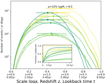
(5) The Astrophysical Journal, 874:117 (10pp), 2019 April 1. Buchner et al.. Figure 5. Left panel: the birth rate of black holes over cosmic time. Curves show different seeding fractions p and mass thresholds M0. Center panel: merger rate of halos occupied by black holes. The kink at z∼1 is due to the simulation’s cosmic variance, i.e., a large overdensity merging at that redshift. Right panel: the total number of halos with black holes. We compare with space densities of AGN with luminosities LX > 3 ´ 10 42 erg s-1 (AGN) and LX > 10 44 erg s-1 (QSOs) measured by X-ray surveys sensitive to unobscured and obscured accretion (Buchner et al. 2015). Comparing the model curves and observations, we see that only a very small fraction (1:10 to 1:10,000) of black holes accrete at these luminosities.. (∼1 instead of ∼0.5). Nevertheless, also in those models, merger delays will shift the GW events to lower redshifts, and thus the LISA diagnostic diagram can diagnose the shift within a particular model. As discussed in Salcido et al. (2016) and Barausse (2012), the number of GW events and their redshift distribution are powerful diagnostics to compare seeding models. The LISA diagnostic diagram, based on (N , A¯ ) or just (N, μ), provides a useful visual summary of model predictions. 6. SMBHs Active As Quasars at z∼6 The earliest census of the SMBH population is available from very high-redshift quasar surveys. The Sloan Digital Sky Survey revealed several dozens of high-redshift optical quasars at z∼6–8 (e.g., Fan et al. 2001; Jiang et al. 2016). Because quasars are interpreted as accreting SMBHs, the quasar number density measurement places a lower limit10 on the black hole volume density. An assumption made by some previous works is that these quasars live in the most massive halos at that time (e.g., Volonteri & Rees 2006; Wyithe & Padmanabhan 2006; Li et al. 2007; Romano-Díaz et al. 2011). This makes it easier for modelers to explain high black hole masses. In this and the next section we explore the consequences of this halo density matching assumption and relax it. Figure 8 shows the observational lower limit as a dotted horizontal line for quasars (Willott et al. 2010b; Jiang et al. 2016) and AGN (Onoue et al. 2017). Well above this, the top-most curve shows the cumulative halo mass function, i.e., the number of halos above a given mass. If quasars populated only the most massive halos, e.g., M>1012.5 Me, the space density would match observations. If instead quasars are permitted to inhabit lower masses, e.g., Mh∼1011 Me, only a very small fraction ( f≈ 10−6, bottom panel) of halos need be quasars. According to our. Figure 6. Distribution of predicted gravitational wave events in log (1 + z ). The 10% seeding of M0 = 108 M halos is shown here as the yellow dashed line. Different delay distributions (inset, from Kelley et al. 2017) shift the distribution to later times, and can reduce the number of events. The error bars show the meanμ and standard deviation σ of the log (1 + z ) distributions, which are combined in Figure 7 as A¯ = m - 4s . The colors indicate the location of the mean. Altering the seeding prescription mostly changes the normalization (see middle panel of Figure 5).. points, from left to right). To quantify Ā with an uncertainty of ±0.05 requires approximately 200 GW detections. We verify that we reproduce the same results as Salcido et al. (2016) under their assumptions (Mc=1010 Me, p=1, no or short delays). In other words, their GW event rates are special cases of our framework. As noted there, however, Sesana et al. (2007) obtained substantially different results, as in their model’s seeding peaks at z∼10 and ends by z∼6. In that case, A¯ > 0 9, because the average log (1 + z ) is higher. 10. It is a lower limit because this selection misses obscured, faint, and dormant black holes, and possibly, by virtue of the Eddington limit, also those with the lowest masses. As shown before, the fraction of dormant SMBH can be very high at least in the local universe, and so is the fraction of obscured AGN (e.g., 75% in Buchner et al. 2015).. 9 Specifically, (N , A¯ ) for their models are VHM: (10.67, 0.143), KBD: (79.75, 0.26), BVRhf: (0.97, 0.076), and BVRlf: (4.93,0.015).. 5.
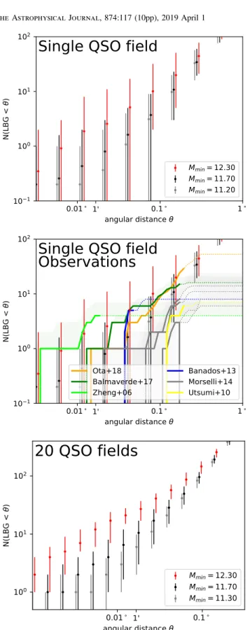
(6) The Astrophysical Journal, 874:117 (10pp), 2019 April 1. Buchner et al.. Figure 7. Gravitational wave diagnostic diagram. The plot axes are observables: the number of GW events per year (y-axis) and a skew statistic of their redshift distribution (x-axis). Points correspond to various seeding models and inspiral delay functions (color-coded by median delay, from Figure 6). Purple contour curves indicate the number of black holes predicted by each model, which strongly influences the GW event rate (y-axis), with limited effect by the delay time. The observable statistic on the x-axis approximately corresponds to the inspiral delay. Models below 1 yr−1 are excluded by current occupation constraints (see Figure 2).. and UDS fields of Hatfield et al. (2018), we use the simple prescription that LBGs occupy halos of M>1011.2 Me, and verify that this matches the number detected in those (non-QSO) fields. Selecting a cylinder as high as the redshift selection (∼500 Mpc) and projecting it, we take into account chance alignments. For each quasar we compute the number of LBGs enclosed within an angular separation of θ. This is shown in the top panel of Figure 9. The mean number is generally higher in the high-mass case (red), but there is substantial overlap in the 95% confidence intervals. This indicates that a single quasar field is not powerful enough to discriminate halo mass occupations, and wide variations of numbers are expected. This is indeed what is observed: Some studies claim overdensities (e.g., Zheng et al. 2006), while others find densities comparable to control fields (e.g., Bañados et al. 2013; Morselli et al. 2014; Mazzucchelli et al. 2017; Ota et al. 2018). In the middle panel of Figure 9 we compiled some studies11 and present as thick curves the enclosed number of LBGs as a function of angular distance. Overall, the data are consistent with all three model ranges at all radii. The Zheng et al. (2006) data set12. seeding prescription, we expect all of these halos to have SMBHs, but their triggering as quasars requires closer investigation. 6.1. Environments of z∼6 Quasars If quasars at z∼6 indeed live in very massive halos, galaxy overdensities should be observable around them. Identifying overdensities has, however, produced contradictory results in the literature. In this section, we use mock observations to understand the difficulties. From the simulations, we can predict the number of galaxies near quasars. For this, we consider three cases for the minimal quasar halo masses in the 3×10¹¹–3×10¹² Me range (squares in the lower panel of Figure 8), and draw 1000 halos randomly above that threshold. For a mock observation, we then search for surrounding galaxy halos, taking into account the angular separation and redshift selection window. We assign galaxies to halos to mimic observations. Lyman break galaxies (LBGs) can be found at these redshifts through filter drop-outs (e.g., Stanway et al. 2003; Zheng et al. 2006; Bouwens et al. 2011; Ota et al. 2018). This selects a relatively broad redshift range (we adopt here z=5.5–7; e.g., Ota et al. 2018) to a typical detection limit of 26th magnitude AB (e.g., Utsumi et al. 2010; Morselli et al. 2014; Ota et al. 2018). Following the LBG clustering analysis in the UltraVISTA. 11. The luminosities of the targets are consistent with the quasar definition used in Figure 8. The LBG magnitude detection limits in these studies are comparable. We have considered their C-complex as a single source and chose those objects only 1σ above their color-cut as less secure candidates.. 12. 6.
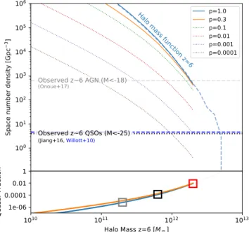
(7) The Astrophysical Journal, 874:117 (10pp), 2019 April 1. Buchner et al. 13. This may indicate that our LAE detect any sources. prescription is too abundant. The bottom panel shows predictions when 10 quasar fields have been observed. In that case, the predictions marginally separate. The LAE and LBG populations are both promising approaches to constrain the halo mass of quasars, and thereby the fraction of black holes active as quasars (Figure 8). However, because dark matter halo neighborhoods are diverse, observations of many quasar fields are needed to make definitive statements.14. 7. Discussion and Conclusion We made an analysis of SMBH seeding that is independent of the seed mass, growth mechanism, and feedback processes, to estimate the number of massive black holes across cosmic time. Our assumption, following Menou et al. (2001), is simply that by the time a dark matter halo reaches a critical mass Mc, some process has seeded it with a black hole with efficiency p. Details of the seeding process involved are not needed in our analysis. The high black holeoccupation fraction observed in local low-mass galaxies constrains these parameters. The seeding fraction p has to exceed p (Mc/1011 Me)3/4 (see Figure 4). This simultaneously constrains the underlying population, for example, the local SMBH space density is above >0.01/Mpc3 in all our models. In our framework, black hole seeding happens continuously throughout cosmic time, but is generally most frequent at z>4. If we require seeding to only occur before the epoch of reionization (z>7), generally lower mass thresholds are required to increase the population (dotted line in Figure 4). However, the merger distributions shift only slightly to higher redshifts. Indeed, when seeding only a small fraction of halos (e.g., p=1%), a redshift cutoff has virtually no effect on the shape of the host merger history. Our framework can approximate the behavior of physically motivated seeding mechanisms. Some examples are shown in Figure 4 for comparison. The light seed scenario of Volonteri et al. (2003) considers the end-products of Population III stars. This mechanism effectively populates all Mc107 Me halos at z∼20 with SMBH seeds, and as such is taken as a special case of our formalism. Heavy seed scenarios operate at higher masses Mc3×107 Me halos at z∼10, but are less efficient (p=3–30, e.g., Volonteri et al. 2008; Agarwal et al. 2012). These require UV radiation from neighboring galaxies, which usually merge after the host halo creates the seed (by z 6, e.g., Agarwal et al. 2014). Their effective behavior may thus perhaps be better approximated with a higher mass threshold with lower efficiencies down to lower redshift. In practice, however, the differences in the model predictions at lower redshift (>1 Gyr after seeding) are negligible. If we apply a z>15 constraint to our seeding prescription this yields very stringent constraints on the parameter space, ruling out Mc109 Me, and giving p20% for Mc=108 Me, the smallest halo masses our simulations can reliably probe. These efficiency constraints are also consistent with Greene (2012), which showed that the aforementioned models are near current observational constraints. In any case, however, all surviving. Figure 8. Top panel: cumulative halo mass function of black hole hosts at z=6. The total cumulative halo mass function (blue curve) provides an upper envelope of the number of hosts available above a given mass (x-axis). At very high masses this is taken from a larger simulation box (dashed). The colored curves represent our results from seeding halos and assuming that quasars occur in halos above a minimum halo mass (x-axis). Surveys of bright quasars find observed space densities of ∼4 Gpc−3 (dashed blue line: Willott et al. 2010b, dotted black line: Jiang et al. 2016). Focusing on p 30%, the ratio between the black hole space density model curve and the observed quasar space density is shown in the bottom panel. The rectangles show the three cases investigated. Red: quasars populate only high-mass halos, black: intermediate, gray: quasars live in >3 ´ 1011 M halos.. could be an exception just where their field of view ends, as well as one of the Morselli et al. (2014) fields at the low end. Clearly, more observations are needed to reduce the variations. The bottom panel of Figure 9 shows model predictions for 20 quasar fields. At this point the most massive scenario can be unambiguously distinguished. Some of the prediction variance is likely due to the broad redshift range of the LBG selection (Δz≈1.5 corresponding to ∼500 Mpc). To focus on the environment near the quasar, studies have advocated the use of Lyman-alpha emitters (LAEs) to complement LBGs studies. To detect the Lyα line near the target quasar redshift requires narrow (and sometimes custom-made) filters, but has the benefit of probing a narrow redshift range (Δz∼0.1). We again adopt a simple prescription, following Kovač et al. (2007) and Sobacchi & Mesinger (2015), and assign LAEs to halos above a halo mass limit of M>1010.6 Me. We verify that the numbers in non-QSO fields, SXDS (Ouchi et al. 2010) and SDF (Ota et al. 2018), are reproduced. These can also be reproduced by choosing a lower mass cut and a duty cycle, but we find this does not change our conclusions significantly. We again compute the enclosed number of neighbors to the quasar at various angular separations. The top panel of Figure 10 shows the predictions, which are indistinguishable for a single quasar field. Observations (middle panel; Bañados et al. 2013; Goto et al. 2017; Mazzucchelli et al. 2017; Ota et al. 2018) fall within the predicted ranges, which are extremely wide, in part due to Poisson statistics. The only measurement falling outside one of the predicted ranges is that of Goto et al. (2017), which did not. 13. This is the same field as the Utsumi et al. (2010) LBG measurement. A related analysis based on hydro-dynamic cosmological simulations was made in Habouzit et al. (2018).. 14. 7.
(8) The Astrophysical Journal, 874:117 (10pp), 2019 April 1. Buchner et al.. Figure 10. LAEs near quasars at z∼6. The number of LAEs enclosed in a given angular distance (e.g., 1arcmin) is plotted. Top panel: for three cases of minimum halo masses of quasar hosts, the frequency of LAEs is predicted. Error bars cover 95% of randomly drawn hosts. The predictions are highly degenerate. Middle panel: observations. Solid curves show the number of observed LAEs and continue as dotted when the edge of the field is reached. The Goto et al. (2017) field (green downward-pointing triangles) did not show any sources. Bottom panel: if 10 quasar fields are observed, the model predictions start to be distinguishable.. Figure 9. LBGs near quasars at z∼6. The number of LBGs enclosed in a given angular distance (e.g., 1 arcmin) is plotted. Top panel: for three cases of minimum halo masses of quasar hosts, the frequency of LBGs is predicted. Error bars cover 95% of randomly drawn hosts. Middle panel: observations. Solid curves show the number of observed LBGs and continue as dotted when the edge of the field is reached. When less secure candidates are included, the numbers may be higher (shading). Bottom panel: if 20 quasar fields are observed, the highest-mass model prediction can be clearly distinguished.. 8.
(9) The Astrophysical Journal, 874:117 (10pp), 2019 April 1. Buchner et al.. resolution θ the black hole sphere of influence is detectable only to distances D » 2.3 Mpc ´ (q 0. 1) ´ MBH 106M (e.g., Do et al. 2014).15 Thus many local galaxies are beyond the resolution limit of current instruments (Ferrarese & Ford 2005), but can hopefully be probed with upcoming Extremely Large Telescopes (Do et al. 2014). Thanks to its sensitivity to black hole mergers of various sizes, LISA will provide the most powerful constraints on the abundance of SMBHs. Figure 7 shows that the number of LISA detections per year correlates with the local black hole number density, which relates to a Mc×p combination (right panel of Figure 5).. 11. models have populated all M>10 Me halos with SMBH seeds at z∼6. The quasar population at z∼6 can also be connected to our prescription. Willott et al. (2010a) argued that the observed z∼6–7 quasars are the MBH>107 Me population accreting at the Eddington limit, while the remaining black holes are pristine seeds without substantial accretion. Under this interpretation we consider f the success fraction of turning a seed into a quasar at that redshift. Indeed, the above constraints indicate that at z∼6, there is an abundance of black holes. Fewer than ∼10−6 of the seeds are quasars at that time. If seeds become SMBH and potential quasars only above a certain halo masses, the active fraction can still be as low as f∼10−5, indicating that we may only see very “lucky” seeds. Thus, our constraints show that physical seeding mechanisms and the activation of quasars can be highly inefficient. For example, when studying a comoving cosmological volume of 20 Mpc side length, the theorist needs to create ∼80 seeds by z≈6, but only one in a million of those need to become a quasar with an SMBH. It is thus encouraging to consider seeding and feeding mechanisms requiring rare conditions, such as special configurations of halos or multiple, complex mergers (see, e.g., Agarwal et al. 2012; Inayoshi et al. 2018; Mayer & Bonoli 2019), rather than focusing on massive halos. Several works have studied overdensities to measure the halo mass of quasars with mixed results. We demonstrate that the diversity of single-QSO field observations is expected. This is because even at a given mass, halos have diverse neighborhoods, with the number of surrounding halos varying by an order of magnitude. Previously, Overzier et al. (2009) came to a similar conclusion considering a mock field observation of i-band dropout galaxies. Observations of several quasar fields are necessary to make definitive statements about the host halo mass of quasars. LBGs and LAEs are both suitable probes. However, given that detection of LAEs requires filters specific to the targeted quasar redshift, observations of LBGs may be more economical. In the clustering predictions we have made highly simplified assumptions, especially in how LAEs and LBGs populate and cluster around halos at high redshift. This is still an open research question also in nonquasar fields. A promising future probe of the seeding scenarios is the space-based LISA gravitational wave experiment (eLISA Consortium et al. 2013), because of its broad mass and redshift sensitivity. We have presented a new diagnostic diagram for LISA GW events. The number of observed events and their redshift distribution can probe simultaneously both the space density of the SMBH population and the typical delay between halo and black hole mergers. We populate the diagram with various seeding scenarios, taking into account possible delays between halo mergers and black hole coalescence, and find that the local SMBH occupation constraints already imply a lower limit of at least one GW event per year detected by LISA. Current SMBH constraints are lower limits on their occurance, as inactive SMBH can often go undetected. To strongly constrain the parameter space, e.g., to near the dashed line in Figure 4, it would be necessary to establish that 50% of the Må∼109 Me galaxies lack an SMBH (under some mass definition of SMBH seeds). This is challenging because with an imaging. J.B. thanks Roberto E. Gonzalez and Nelson D. Padilla for feedback on the manuscript. We acknowledge support from the CONICYT-Chile grants Basal-CATA PFB-06/2007 and Basal AFB-170002 (J.B., F.E.B., E.T.), FONDECYT Regular 1141218 (F.E.B.) and 1160999 (E.T.), FONDECYT Postdoctorados 3160439 (J.B.), CONICYT PIA Anillo ACT172033 (E.T.), and the Ministry of Economy, Development, and Tourism’s Millennium Science Initiative through grant IC120009, awarded to The Millennium Institute of Astrophysics, MAS (J.B., F.E.B.). L.F.S. and K.S. acknowledge support from SNSF Grants PP00P2_138979 and PP00P2_166159. A discussion of some aspects of this work was carried out at the Aspen Center for Physics, which is supported by National Science Foundation grant PHY-1607611. The authors gratefully acknowledge the Gauss Centre for Supercomputing e.V. (www.gauss-center.eu) and the Partnership for Advanced Supercomputing in Europe (PRACE,www. prace-ri.eu) for funding the MultiDark simulation project by providing computing time on the GCS Supercomputer SuperMUC at Leibniz Supercomputing Centre (LRZ,www.lrz.de). The MultiDark simulations were performed on the Pleiades supercomputer at the NASA Ames supercomputer center. The SMDPL simulations have been performed on SuperMUC at LRZ in Munich within the pr87yi project. The MultiDark Database used in this paper and the web application providing online access to it were constructed as part of the activities of the German Astrophysical Virtual Observatory as result of a collaboration between the Leibniz-Institute for Astrophysics Potsdam (AIP) and the Spanish MultiDark Consolider Project CSD2009-00064. The Geryon cluster at the Centro de AstroIngenieria UC was extensively used for the FORS simulation. The Anillo ACT-86, FONDEQUIP AIC-57, and QUIMAL 130008 11 provided funding for several improvements to the Geryon cluster. ORCID iDs Johannes Buchner https://orcid.org/0000-0003-0426-6634 Ezequiel Treister https://orcid.org/0000-0001-7568-6412 Franz E. Bauer https://orcid.org/0000-0002-8686-8737 Kevin Schawinski https://orcid.org/0000-0001-5464-0888 References Agarwal, B., Dalla Vecchia, C., Johnson, J. L., Khochfar, S., & Paardekooper, J.-P. 2014, MNRAS, 443, 648 Agarwal, B., Khochfar, S., Johnson, J. L., et al. 2012, MNRAS, 425, 2854 Amaro-Seoane, P., Audley, H., Babak, S., et al. 2017, arXiv:1702.00786 15 This contains MBH∝σ4; however, the relation is uncertain at low masses (see, e.g., Kormendy & Ho 2013; Graham 2016).. 9.
(10) The Astrophysical Journal, 874:117 (10pp), 2019 April 1. Buchner et al.. Bañados, E., Venemans, B., Walter, F., et al. 2013, ApJ, 773, 178 Barausse, E. 2012, MNRAS, 423, 2533 Behroozi, P. S., Wechsler, R. H., & Wu, H.-Y. 2013a, ApJ, 762, 109 Behroozi, P. S., Wechsler, R. H., Wu, H.-Y., et al. 2013b, ApJ, 763, 18 Bouwens, R. J., Illingworth, G. D., Oesch, P. A., et al. 2011, ApJ, 737, 90 Buchner, J., Georgakakis, A., Nandra, K., et al. 2015, ApJ, 802, 89 Crain, R. A., Schaye, J., Bower, R. G., et al. 2015, MNRAS, 450, 1937 Croton, D. J., Springel, V., White, S. D. M., et al. 2006, MNRAS, 365, 11 Croton, D. J., Stevens, A. R. H., Tonini, C., et al. 2016, ApJS, 222, 22 Desroches, L.-B., & Ho, L. C. 2009, ApJ, 690, 267 Do, T., Wright, S. A., Barth, A. J., et al. 2014, AJ, 147, 93 eLISA Consortium, Amaro Seoane, P., Aoudia, S., et al. 2013, (arXiv:1305.5720) Fan, X., Narayanan, V. K., Lupton, R. H., et al. 2001, AJ, 122, 2833 Ferrarese, L., & Ford, H. 2005, SSRv, 116, 523 González, R. E., & Padilla, N. D. 2016, ApJ, 829, 58 Goto, T., Utsumi, Y., Kikuta, S., et al. 2017, MNRAS, 470, L117 Graham, A. W. 2016, in Galactic Bulges, Astrophysics and Space Science Library Vol. 418, ed. E. Laurikainen, R. Peletier, & D. Gadotti (Cham: Springer International Publishing), 263 Greene, J. E. 2012, NatCo, 3, 1304 Habouzit, M., Volonteri, M., Somerville, R. A., et al. 2018, MNRAS, submitted (arXiv:1810.11535) Hatfield, P. W., Bowler, R. A. A., Jarvis, M. J., & Hale, C. L. 2018, MNRAS, 477, 3760 Inayoshi, K., Li, M., & Haiman, Z. 2018, MNRAS, 479, 4017 Jiang, L., McGreer, I. D., Fan, X., et al. 2016, ApJ, 833, 222 Kelley, L. Z., Blecha, L., & Hernquist, L. 2017, MNRAS, 464, 3131 Klypin, A., Yepes, G., Gottlöber, S., Prada, F., & Heß, S. 2016, MNRAS, 457, 4340 Kormendy, J., & Ho, L. C. 2013, ARA&A, 51, 511 Kovač, K., Somerville, R. S., Rhoads, J. E., Malhotra, S., & Wang, J. 2007, ApJ, 668, 15 Latif, M. A., & Ferrara, A. 2016, PASA, 33, e051 Li, Y., Hernquist, L., Robertson, B., et al. 2007, ApJ, 665, 187 Marconi, A., Risaliti, G., Gilli, R., et al. 2004, MNRAS, 351, 169 Mayer, L., & Bonoli, S. 2019, RPPh, 82, 016901 Mazzucchelli, C., Bañados, E., Decarli, R., et al. 2017, ApJ, 834, 83. Menou, K., Haiman, Z., & Narayanan, V. K. 2001, ApJ, 558, 535 Miller, B. P., Gallo, E., Greene, J. E., et al. 2015, ApJ, 799, 98 Morselli, L., Mignoli, M., Gilli, R., et al. 2014, A&A, 568, A1 Moster, B. P., Somerville, R. S., Maulbetsch, C., et al. 2010, ApJ, 710, 903 Naab, T., & Ostriker, J. P. 2017, ARA&A, 55, 59 Onoue, M., Kashikawa, N., Willott, C. J., et al. 2017, ApJL, 847, L15 Ota, K., Venemans, B. P., Taniguchi, Y., et al. 2018, ApJ, 856, 109 Ouchi, M., Shimasaku, K., Furusawa, H., et al. 2010, ApJ, 723, 869 Overzier, R. A., Guo, Q., Kauffmann, G., et al. 2009, MNRAS, 394, 577 Planck Collaboration, Ade, P. A. R., Aghanim, N., et al. 2014, A&A, 571, A16 Prada, F., Klypin, A. A., Cuesta, A. J., Betancort-Rijo, J. E., & Primack, J. 2012, MNRAS, 423, 3018 Rees, M. J. 1984, ARA&A, 22, 471 Reines, A. E., & Comastri, A. 2016, PASA, 33, e054 Romano-Díaz, E., Choi, J.-H., Shlosman, I., & Trenti, M. 2011, ApJL, 738, L19 Salcido, J., Bower, R. G., Theuns, T., et al. 2016, MNRAS, 463, 870 Sawala, T., Frenk, C. S., Crain, R. A., et al. 2013, MNRAS, 431, 1366 Schaye, J., Crain, R. A., Bower, R. G., et al. 2015, MNRAS, 446, 521 Sesana, A., Haardt, F., Madau, P., & Volonteri, M. 2004, ApJ, 611, 623 Sesana, A., Volonteri, M., & Haardt, F. 2007, MNRAS, 377, 1711 Sobacchi, E., & Mesinger, A. 2015, MNRAS, 453, 1843 Soltan, A. 1982, MNRAS, 200, 115 Somerville, R. S., & Davé, R. 2015, ARA&A, 53, 51 Stanway, E. R., Bunker, A. J., & McMahon, R. G. 2003, MNRAS, 342, 439 Utsumi, Y., Goto, T., Kashikawa, N., et al. 2010, ApJ, 721, 1680 Volonteri, M. 2010, A&ARv, 18, 279 Volonteri, M., Haardt, F., & Madau, P. 2003, ApJ, 582, 559 Volonteri, M., Lodato, G., & Natarajan, P. 2008, MNRAS, 383, 1079 Volonteri, M., & Rees, M. J. 2006, ApJ, 650, 669 Weinberger, R., Springel, V., Pakmor, R., et al. 2018, MNRAS, 479, 4056 Willott, C. J., Albert, L., Arzoumanian, D., et al. 2010a, AJ, 140, 546 Willott, C. J., Delorme, P., Reylé, C., et al. 2010b, AJ, 139, 906 Wyithe, J. S. B., & Padmanabhan, T. 2006, MNRAS, 366, 1029 Yu, Q., & Tremaine, S. 2002, MNRAS, 335, 965 Zheng, W., Overzier, R. A., Bouwens, R. J., et al. 2006, ApJ, 640, 574. 10.
(11)
Figure
+4
Documento similar
In this respect, a comparison with The Shadow of the Glen is very useful, since the text finished by Synge in 1904 can be considered a complex development of the opposition
The Dwellers in the Garden of Allah 109... The Dwellers in the Garden of Allah
that when looking at the formal and informal linguistic environments in language acquisition and learning it is necessary to consider the role of the type of
Since such powers frequently exist outside the institutional framework, and/or exercise their influence through channels exempt (or simply out of reach) from any political
In this article we compute explicitly the first-order α 0 (fourth order in derivatives) corrections to the charge-to-mass ratio of the extremal Reissner-Nordstr¨ om black hole
Of special concern for this work are outbreaks formed by the benthic dinoflagellate Ostreopsis (Schmidt), including several species producers of palytoxin (PLTX)-like compounds,
In the previous sections we have shown how astronomical alignments and solar hierophanies – with a common interest in the solstices − were substantiated in the
While Russian nostalgia for the late-socialism of the Brezhnev era began only after the clear-cut rupture of 1991, nostalgia for the 1970s seems to have emerged in Algeria
