The 31 Deg2 Release of the Stripe 82 X Ray Survey: The Point Source Catalog

Texto completo

(1)The Astrophysical Journal, 817:172 (21pp), 2016 February 1. doi:10.3847/0004-637X/817/2/172. © 2016. The American Astronomical Society. All rights reserved.. THE 31 DEG2 RELEASE OF THE STRIPE 82 X-RAY SURVEY: THE POINT SOURCE CATALOG Stephanie M. LaMassa1,2,3, C. Megan Urry1,2, Nico Cappelluti4, Hans Böhringer5, Andrea Comastri4, Eilat Glikman6, Gordon Richards7, Tonima Ananna1,2, Marcella Brusa4,8, Carie Cardamone9, Gayoung Chon5, Francesca Civano1,10, Duncan Farrah11, Marat Gilfanov12,13, Paul Green10, S. Komossa14, Paulina Lira15, Martin Makler16, Stefano Marchesi1,4,10, Robert Pecoraro1,2, Piero Ranalli4,17, Mara Salvato5, Kevin Schawinski18, Daniel Stern19, Ezequiel Treister20, and Marco Viero21,22 1. Yale Center for Astronomy & Astrophysics, Physics Department, P.O. Box 208120, New Haven, CT 06520, USA 2 Department of Physics, Yale University, P.O. Box 208121, New Haven, CT 06520, USA 3 Now at NASA Goddard Space Flight Center, Greenbelt, MD 20771, USA 4 INAF-Osservatorio Astronomico di Bologna, via Ranzani 1, I-40127 Bologna, Italy 5 Max-Planck-Institut für extraterrestrische Physik, D-85748 Garching, Germany 6 Department of Physics, Middlebury College, Middlebury, VT 05753, USA 7 Department of Physics, Drexel University, 3141 Chestnut Street, Philadelphia, PA 19104, USA 8 DIFADipartimento di Fisica e Astronomia, Universita’ di Bologna, viale Berti Pichat 6/2, I-40127 Bologna, Italy 9 Department of Math & Science, Wheelock College, 200 Riverway, Boston, MA 02215, USA 10 Smithsonian Astrophysical Observatory, 60 Garden Street, Cambridge, MA 02138, USA 11 Department of Physics MC 0435, Virginia Polytechnic Institute and State University, 850 West Campus Drive, Blacksburg, VA 24061, USA 12 Max-Planck Institut für Astrophysik, Karl-Schwarzschild-Str. 1, Postfach 1317, D-85741 Garching, Germany 13 Space Research Institute of Russian Academy of Sciences, Profsoyuznaya 84/32, 117997 Moscow, Russia 14 Max-Planck-Institut für Radioastronomie, Auf dem Hügel 69, D-53121 Bonn, Germany 15 Departamento de Astronomia, Universidad de Chile, Camino del Observatorio 1515, Santiago, Chile 16 ́ Centro Brasileiro de Pesquisas Fisicas, Rua Dr Xavier Sigaud 150, Rio de Janeiro, RJ 22290-180, Brazil 17 Institute for Astronomy, Astrophysics, Space Applications and Remote Sensing (IAASARS), National Observatory of Athens, 15236 Penteli, Greece 18 Institute for Astronomy, Department of Physics, ETH Zurich, Wolfgang-Pauli Strasse 27, CH-8093 Zurich, Switzerland 19 Jet Propulsion Laboratory, California Institute of Technology, Pasadena, CA 91109, USA 20 Department of Astronomy, University of Concepcion, Concepcion, Chile 21 Kavli Institute for Particle Astrophysics and Cosmology, Stanford University, 382 Via Pueblo Mall, Stanford, CA 94305, USA 22 California Institute of Technology, 1200 E. California Boulevard, Pasadena, CA 91125, USA Received 2015 September 29; accepted 2015 November 28; published 2016 February 1. ABSTRACT We release the next installment of the Stripe 82 X-ray survey point-source catalog, which currently covers 31.3 deg2 of the Sloan Digital Sky Survey (SDSS) Stripe 82 Legacy field. In total, 6181 unique X-ray sources are significantly detected with XMM-Newton (>5σ) and Chandra (>4.5σ). This catalog release includes data from XMM-Newton cycle AO 13, which approximately doubled the Stripe 82X survey area. The flux limits of the Stripe 82X survey are 8.7×10−16 erg s−1 cm−2, 4.7×10−15 erg s−1 cm−2, and 2.1×10−15 erg s−1 cm−2 in the soft (0.5–2 keV), hard (2–10 keV), and full bands (0.5–10 keV), respectively, with approximate half-area survey flux limits of 5.4×10−15 erg s−1 cm−2, 2.9×10−14 erg s−1 cm−2, and 1.7×10−14 erg s−1 cm−2. We matched the X-ray source lists to available multi-wavelength catalogs, including updated matches to the previous release of the Stripe 82X survey; 88% of the sample is matched to a multi-wavelength counterpart. Due to the wide area of Stripe 82X and rich ancillary multi-wavelength data, including coadded SDSS photometry, mid-infrared WISE coverage, near-infrared coverage from UKIDSS and VISTA Hemisphere Survey, ultraviolet coverage from GALEX, radio coverage from FIRST, and far-infrared coverage from Herschel, as well as existing ∼30% optical spectroscopic completeness, we are beginning to uncover rare objects, such as obscured high-luminosity active galactic nuclei at high-redshift. The Stripe 82X point source catalog is a valuable data set for constraining how this population grows and evolves, as well as for studying how they interact with the galaxies in which they live. Key words: catalogs – galaxies: active – quasars: general – surveys – X-rays: general Supporting material: FITS files 1. INTRODUCTION. mid-infrared emission from AGN heated circumnuclear dust (Spinoglio & Malkan 1989; Lacy et al. 2004; Stern et al. 2005; Donley et al. 2012; Stern et al. 2012; Assef et al. 2013), and fine-structure emission lines (Farrah et al. 2007; Weaver et al. 2010; Meléndez et al. 2014), and radio emission from jets launched by the accretion disk (Kellermann et al. 1989; Hooper et al. 1995). These different selection criteria favor different parts of the AGN population, and by combining these methods, a comprehensive view of black hole growth is revealed. Multi-wavelength surveys are then the key for unlocking the secrets of AGN evolution and how they relate to the galaxies they inhabit. Complementary survey strategies select different. Active galactic nuclei (AGNs) signal the growth of supermassive black holes at galactic centers. Studying AGNs over a range of redshift allows us to discover how supermassive black holes evolve over cosmic time to the present day. As AGNs emit energy over a range of wavelengths, they can be identified by various signatures, including optical and ultraviolet light from the accretion disk feeding the black hole (Koratkar & Blaes 1999), optical emission from gas ionized by accretion disk photons (Baldwin et al. 1981; Veilleux & Osterbrock 1987; Vanden Berk et al. 2001), X-ray emission from the AGN corona (Haardt & Maraschi 1991; Brandt & Alexander 2015), 1.

(2) The Astrophysical Journal, 817:172 (21pp), 2016 February 1. LaMassa et al.. populations in the redshift-luminosity plane. Deep, pencilbeam surveys uncover the faintest objects in the universe while wide-area surveys are required to discover a representative sampling of rare objects that have a low space density. Such rare sources include high-luminosity AGNs at high-redshift (e.g., Lx>1045 erg s−1 at z>2), which, according to current theories, are the phases when most of the mass locked up in current black holes was accreted (e.g., Hopkins & Hernquist 2009; Treister et al. 2012). Wide-area surveys have existed for years at optical, infrared, and radio wavelengths, but have only recently been underway in X-rays at energies above 2 keV and at depths capable of pushing to cosmological distances. While the deep, small area Chandra Deep Field South Survey (0.13 deg2; Giacconi et al. 2001; Xue et al. 2011) has uncovered the faintest AGNs and has entered the flux regime where the number density of non-active galaxies surpasses that of active systems (Lehmer et al. 2012), and medium-area surveys like XMM-Newton and Chandra-COSMOS (2.2 deg2; Cappelluti et al. 2007; Hasinger et al. 2007; Elvis et al. 2009; Brusa et al. 2010; Civano et al. 2012, 2015; Marchesi et al. 2015) have identified nearly 2,000 moderate-luminosity AGNs (1043 erg s−1<Lx< 1044 erg s−1), the Lx>1045 erg s−1 population has been a missing tier in our hard X-ray census of supermassive black hole growth. This population began to be revealed with larger area (∼10 deg2) surveys, such as XBoötes (9 deg2; Kenter et al. 2005; Murray et al. 2005) and the Chandra Multi-wavelength Project (ChaMP, 10 deg2; Kim et al. 2007), as well as the more recent XMM-Newton survey in the Herschel ATLAS field (7.1 deg2; Ranalli et al. 2015). The advent of the widest-area surveys (>15 deg2), including the “Stripe 82X” survey (LaMassa et al. 2013a, 2013b), which, as we discuss below, now reaches ∼31.3 deg2, as well as the 50 deg2XMM-XXL (PI: Pierre) and the ∼877 deg2XMM-Serendipitous (Rosen et al. 2015) surveys, provides a chance to study the evolution of the most luminous AGN in unprecedented detail. However, though the XMM-Serendipitous survey covers an order of magnitude more area than the dedicated large-area XMMNewton surveys, an important component is missing: supporting multi-wavelength data which allows the X-ray photons to be identified with discrete sources and the properties of these objects to be characterized. A field which contains such supporting information, such as the Sloan Digital Sky Survey (SDSS; York et al. 2000) Stripe 82 region, is therefore an ideal location to execute an X-ray survey with maximal efficiency for returning comprehensive results. Stripe 82 is a 300 deg2 equatorial region imaged between 80 and 120 times as part of a supernova survey with SDSS (Frieman et al. 2008). The coadded photometry reaches 1.2–2.2 magnitudes deeper than any single SDSS scan (r∼24.6 versus r∼22.2; Annis et al. 2014; Jiang et al. 2014), and the full field has existing optical spectroscopy from SDSS and SDSS BOSS (Data Releases 9 and 10; Ahn et al. 2012, 2014), 2 SLAQ (Croom et al. 2009), and WiggleZ (Drinkwater et al. 2010), with partial coverage from DEEP2 (Newman et al. 2013), PRIMUS (Coil et al. 2011), 6dF (Jones et al. 2004, 2009), the VIMOS VLT Deep Survey (VVDS Garilli et al. 2008), a deep spectroscopic survey of faint quasars from Jiang et al. (2006), and a pre-BOSS pilot survey using Hectospec on MMT (Ross et al. 2012). Existing multi-wavelength data in Stripe 82 include near-infrared observations from UKIDSS (Hewett et al. 2006; Casali et al. 2007; Lawrence et al. 2007) and the. Figure 1. Distribution of archival Chandra observations (black diamonds), archival XMM-Newton observations (blue squares), XMM-Newton AO10 observations (blue diamonds), and XMM-Newton AO13 observations (red circles) for the full Stripe 82 region (top) and the XMM-Newton AO13 area (bottom). The symbol size is to scale with the field of view for the AO13 pointings in the bottom panel only.. VISTA Hemisphere Survey (VHS; McMahon et al. 2013); farinfrared coverage from Herschel over 79 deg2 (Viero et al. 2014); ultraviolet coverage with GALEX (Morrissey et al. 2007); radio observations at 1.4 GHz with Faint Images of the Radio Sky at Twenty centimeters (FIRST) (Becker et al. 1995; White et al. 1997; Becker et al. 2012; Helfand et al. 2015), with deeper VLA coverage over 80 deg2 (Hodge et al. 2011); and millimeter observations with the Atacama Cosmology Telescope (ACT; Fowler et al. 2007; Swetz et al. 2011). Additionally, there is Spitzer coverage in the field from the Spitzer-HETDEX Exploratory Large Area survey over 28 deg2 (SHELA; PI: C. Papovich) and the Spitzer IRAC Equatorial Survey over 110 deg2 (SpIES; PI: G. Richards; J. Timlin et al. 2015, in preparation), deeper near-infrared J and K band coverage, to limits of 22 mag (AB), from the VISTACFHT Stripe 82 Survey over 140 deg2 (VICS82, PIs: Geach, Lin, Makler; J. Geach et al. 2015, in preparation), and midinfrared coverage from the all-sky WISE mission (Wright et al. 2010). To take advantage of this rich multi-wavelength coverage, we designed the wide-area Stripe 82X survey (LaMassa et al. 2013a, 2013b) to uncover a representative population of rare, high-luminosity AGNs at high redshift. Here we release the next installment of the Stripe 82X point-source catalog, which includes data awarded to our team in response to XMMNewton Announcement Opportunity 13 (“AO13”), representing ∼980 ks of observing time (PI: C. M. Urry; Proposal ID 074283). We also publish updated catalogs from our previous Stripe 82X data releases from archival Chandra and XMM-Newton observations in Stripe 82 (LaMassa et al. 2013a, 2013b) and a pilot XMM-Newton program granted to our team in AO10 (PI: C. M. Urry; LaMassa et al. 2013a). The positions of the X-ray pointings used in Stripe 82X are shown in Figure 1. In Section 2, we discuss the data analysis for XMM-Newton AO13, which we then combine with the previously released Chandra and XMM-Newton data in Section 3 to characterize the Stripe 82 X-ray survey to date, currently spanning ∼31.3 deg2 of non-overlapping area. In Section 4, we match the X-ray source lists to publicly available catalogs from SDSS, WISE, UKIDSS, VHS, GALEX, FIRST, and Herschel. Throughout, we adopt a cosmology of H0=70 km s−1 Mpc−1, ΩM=0.27, and Λ=0.73. 2.

(3) The Astrophysical Journal, 817:172 (21pp), 2016 February 1. LaMassa et al.. Table 1 XMM-Newton AO13 Observation Summary ObsID. Observation Date. Center R.A.. Center decl.. Discarded Pseudo-exposures. 0742830101 0747390101 0747400101 0747410101 0747420101. 2014 2014 2014 2015 2015. 00:57:23.99 01:05:23.99 01:13:24.00 01:21:24.00 01:29:23.99. −00:22:30.0 −00:22:30.0 −00:22:30.0 −00:22:30.0 −00:22:30.0. 0747430101 0747440101. 2014 Jul 2014 Aug. 01:37:23.99 01:45:23.99. −00:22:30.0 −00:22:30.0. K 22 (PN, M1, M2) K 6 (PN), 8 (PN), 13 (PN) 16 (PN, M1, M2), 18 (PN, M1, M2) 20 (PN, M1, M2), 21 (PN, M1, M2) 22 (PN, M1, M2) 22 (PN, M1, M2). Jul Jul Jul Jan Jan. Area (deg2) 2.33 2.22 2.33 2.32 1.95 2.22 2.22. While this method produced cleaned events files for most of the pseudo-exposures, it did a poor job in instances of intense flaring: a 3σ-clipping was inadequate since the count rate distributions have an extended tail within the 3σ tolerance level. For these pointings, we inspected the count rate distributions by eye to determine a cut-off value to remove the tail of this distribution, visually inspecting both sets of GTIfiltered events files to assess which filtering best removed the background to enhance signal from the sources. Finally, we note that some pseudo-exposures were badly hampered by flaring such that no GTI filtering could recover useful signal. In Table 1, we note which pseudo-exposures were subsequently discarded from our analysis, and whether this affected just the PN detector or all three detectors. We also indicate the effective area covered by each observation after removing flared pointings.. 2. XMM-Newton AO13 OBSERVATIONS AND DATA ANALYSIS Our XMM-Newton AO13 program was executed between 2014 July and 2015 January in a series of seven observations, as summarized in Table 1. Each observation consists of 22 individual pointings, or pseudo-exposures, which were carried out in “mosaic mode.” This observing mode efficiently surveys a large area with individual pointings that have relatively short exposure times. To reduce overhead, the EPIC offset tables are only uploaded (for the MOS detectors) and calculated (for the PN detector) for the first pointing in the series. In our AO13 program, each pseudo-exposure is separated by a half field of view (~15¢) to enable a greater depth to be achieved in the overlapping regions. The median exposure time for individual pointings before filtering is ∼5.2 ks for MOS1 and MOS2 and ∼4.7 ks for PN, while the coadded depth in the overlapping observations reaches ∼6–8 ks after filtering and correcting for vignetting (i.e., the energy-dependent decrease in effective area with off-axis distance). The observational data files (ODF) were generated using the Science Analysis System (SAS) tasks (HEASOFT v. 6.16) emproc and epproc to create the MOS1, MOS2, PN, and PN out-of-time (OoT) events files. The OoT events occur from photons that are detected during CCD readout and recorded at random positions along the readout column. This effect is most significant for the PN detector and affects ∼6.3% of the observing time. The PN images can be statistically corrected for this effect using the PN OoT files. The mosaicked observations were separated into individual pseudo-exposures using the SAS package emosaic_prep. Each pseudo-exposure was then filtered as described below.. 2.2. Generating Products for Source Detection We extracted images from the GTI-filtered events files, using all valid events (PATTERN 0 to 12) for MOS1 and MOS2 and single to double events (PATTERN 0 to 4) for PN. We excluded the energy range from 1.45 to 1.54 keV to avoid the Al Kα line (1.48 keV) from the detector background. The PN detector also has background emission lines from Cu at ∼7.4 and ∼8.0 keV, so we excluded the energy ranges from 7.2 to 7.6 keV and 7.8 to 8.2 keV when extracting PN images. To correct for the OoT events, the PN OoT images were scaled by 0.063 and subtracted from the PN images. We then extracted MOS and PN images in the standard soft (0.5–2 keV), hard (2–10 keV), and full (0.5–10 keV) energy ranges and coadded the images among the detectors. Exposure maps, which quantify the effective exposure time at each pixel in the detector, accounting for vignetting, were generated with the SAS task eexpmap for each detector and energy range. Since vignetting is a strong function of energy, we spectrally weighted the exposure maps such that the mean effective energy inputted into eexpmap is determined by assuming a power-law model where Γ=2.0 in the soft band and Γ=1.7 for the hard and full bands (see Cappelluti et al. 2007). This spectral model was also used to calculate energy conversion factors (ECFs) to convert from count rates to flux, as summarized in Table 2 (for a discussion of how different assumptions for Γ affect the derived ECF, see Loaring et al. 2005; Cappelluti et al. 2007; Ranalli et al. 2013). The exposure maps were coadded among the detectors, weighted by their ECFs. As described in detail by LaMassa et al. (2013a), we used the algorithm presented in Cappelluti et al. (2007) to create background maps. In brief, a simple source detection was run. 2.1. Flare Filtering Episodes of high levels of background radiation cause flaring in the XMM-Newton events files, hampering signal detection amidst the noise. To create good time intervals (GTIs), i.e., selecting events from observation periods where flaring is minimal, we started with a statistical approach. We created histograms of the count rate at high energies, 10–12 keV for the MOS detectors and 10–14 keV for the PN detector, in time bins of 100 s, extracted from single events (PATTERN==0). We created GTIs by excluding periods where the count rate was 3s above the mean and applied this filtering to the events file. From this events file, we searched for periods of low-energy (0.3–10 keV) flares, created GTIs from time bins where the count rate was below 3σ of the mean, and applied this GTI file to the original events file. 3.

(4) The Astrophysical Journal, 817:172 (21pp), 2016 February 1. LaMassa et al.. observation could be fit simultaneously. We therefore executed the source detection in batches, where adjacent columns in R. A. were fit simultaneously. To achieve the greatest coadded depth in the overlapping pointings, each column, other than the eastern and western edges of the mosaic, was included in two source detection runs. We note that the deepest overlap regions are fitted with this source-detection method. The source detection was also run separately for the different energy bands: soft (0.5–2 keV), hard (2–10 keV), and full (0.5–10 keV).. Table 2 Energy Conversion Factors (ECFs)a Band. PN. MOS. Soft (0.5–2 keV) Hard (2–10 keV) Full (0.5–10 keV). 7.45 1.22 3.26. 2.00 0.45 0.97. Note. ECFs in units of counts s−1/10−11 erg cm−2 s−1. These are based on a spectral model where NH=3×1020 cm−2 and Γ=2.0 in the soft band and Γ=1.7 in the hard and full bands. The PN ECF takes into account energy ranges that were masked out due to detector background line emission. a. 2.4. Source List Generation From the above procedure, we have six source lists per energy band per observation. Each list contains duplicate detections of some sources due to the overlapping regions covered in consecutive source detection runs. To produce a clean X-ray source list for each observation, we removed these duplicate detections. Following the algorithm used by the XMM-Newton Serendipitous Source Catalog (Watson et al. 2009) to flag duplicate observations, we consider objects from source lists covering overlapping areas to be the same if the distance between them is less than dcutoff, where (0.9×dnn1, 0.9×dnn2, 15″, dcutoff=min 3×( ra_dec_err12 + sys_err 2 + ra_dec_err 22 + sys_err 2 )), where d nn1 (d nn2 ) is the distance between the source and its nearest neighbor in the first (second) source list, ra_dec_err is the X-ray positional error reported by emldetect, and sys_err is a systematic positional error, taken to be 1″, to account for the sources not having an external astrometric correction applied. A maximum search radius of 15″ was chosen as the maximum cut-off distance based on simulations discussed in LaMassa et al. (2013a), where we found that this radius maximizes identification of output to input sources while minimizing spurious associations of distinct sources; due to the shallow nature of our observations, source confusion from a high density of unresolved sources is not a concern (see Section 3 for estimated source confusion rate). For duplicate detections of the same source, we retain the coordinates, flux, and count information for the object that has the highest detection probability, or det_ml. We perform this routine separately for each energy band, producing one clean source list per band. We then merge these X-ray source lists for each energy band of an observation using the search criterion defined above to find matches among lists generated in the separate energy bands. If no match is found, the source is considered undetected in that band and its flux, flux error, counts, and det_ml are set to null while we retain this information for the band(s) where it is detected. While we have discarded sources that are extended in all bands in which they are detected, because the identification of clusters among the extended sources is in progress and will be reported later, we have flagged the sources that are point-like in one band and are extended in another band. The “ext_flag” is non-zero for these objects and is defined as follows: 1—extended in the soft band, 2—extended in the full band, 3—extended in the hard band, 4 —extended in the soft and full bands, 5—extended in the soft and hard bands, 6—extended in the hard and full bands. To produce the final catalog, the coordinates are averaged among the coordinates from the individual energy band catalogs and their positional errors are added in quadrature; we note that the significance of the detection is not taken into account when averaging the coordinates, but the uncertainty in. on each detector image in each energy band using the SAS task eboxdetect with a low detection probability (likemin=4). The positions of these sources were masked out. The remaining emission results from unresolved cosmic X-ray sources and local particle and detector background. These components were modeled and fit as discussed in Cappelluti et al. (2007) and LaMassa et al. (2013a) to produce a background map for each detector and energy range. The resulting background maps were then coadded among the detectors. Before importing these products into the source detection software, we updated the header keywords “RA_NOM,” “DEC_NOM,” “EXP_ID,” and “INSTRUME” to common values among the pseudo-exposures for each observation: the SAS source detection software, when running on these files simultaneously, will fail if the pseudo-exposures do not have common WCS, exposure ID, and instrument values. However, the “RA_PNT” and “DEC_PNT” header keywords were manually updated to reflect the central coordinates of each pseudo-exposure so that the point spread function (PSF) is correctly calculated during source detection. Detector masks were created using the SAS program emask, which uses the exposure map as input to determine which pixels are active for source detection. 2.3. Source Detection We produced a preliminary list of sources by running the SAS task eboxdetect in “map” mode. This is a sliding-box algorithm that is run on the coadded images, background maps, exposure maps, and detector masks, where source counts are detected in a 5×5 pixel box with a low-probability threshold (likemin=4). This list is then used as an input into emldetect, which performs a maximum likelihood PSF fit to the eboxdetect sources. We used a minimum likelihood threshold (det_ml) of 6, where det_ml=−lnPrandom , where Prandom is the Poissonian probability that a detection is due to random fluctuations. We also included a fit to mildly extended sources, where emldetect convolves the PSF with a β model profile. We consider a source extended if the output ext_flag exceeds 0. Finally, the ECFs reported in Table 2 were summed among the detectors included in the coadded pseudo-exposures (i.e., if the PN image was discarded due to flaring, the ECF sum is from the MOS detectors, while the PN ECF is included in the sum when all detectors are useable), such that emldetect reports the flux in physical units, as well as the count rates, for each detected source. We ran the source detection algorithm separately for each observation. Due to the limited memory capabilities of the SAS source detection software, not all pseudo-exposures within an 4.

(5) The Astrophysical Journal, 817:172 (21pp), 2016 February 1. LaMassa et al.. the astrometric precision is included by adding the positional errors in quadrature. We then retain only objects where det_ml exceeds 15 (i.e., >5σ) in at least one energy band (see Loaring et al. 2005; Mateos et al. 2008, for a discussion of det_ml limits and their effects on Eddington bias in the derived Log N–Log S relation). We caution that care must be taken when determining the reliability of the reported fluxes, as the catalog includes the emldetect reported fluxes for every band where the source was detected (i.e., det _ml  6). Though the X-ray source can be considered a significant detection, as det_ml has to exceed 15 in at least one energy band for the source to be included in the catalog, the det_ml value for each band ought to be used to determine whether the reported flux is at an acceptable significance level. For reference, we use only fluxes in the subsequent analysis when det _ml  15 in that band. Finally, we assign each X-ray source a unique record number (“rec_no”), ranging from 2359 to 5220, since the previous XMM-Newton Stripe 82X catalog release terminated at “rec_no” 2358. We also include columns “in_chandra” and “in_xmm” to note whether a source was detected in the archival Chandra or XMM-Newton Stripe 82X catalogs, respectively, as well as the corresponding identification number of the matched source; for the one XMM-Newton source that has two possible Chandra counterparts within the search radius (rec_no 3473), due to Chandraʼs superior spatial resolution, we list both of the Chandra matches. Details about each column are summarized in the Appendix.. detection rate for the XMM-Newton AO13 data to be 1.0%, 0.67%, and 0.33% in the soft, hard, and full bands, respectively. Furthermore, we can estimate the confusion fraction, which is when input sources are unresolved in the source detection and observed as one object. As we did in LaMassa et al. (2013a), we followed the prescription in Cappelluti et al. (2007) to test for source confusion, using the criterion Sout/(Sin + 3sout ) >1.5, where Sout is the output flux, Sin is the input flux, and σout is the emldetect-reported flux error. According to this metric, the source confusion rate is 0.15%, 0.10%, and 0.16% percent in the soft, hard, and full bands, respectively. To determine survey sensitivity, we generate histograms of all input fluxes and output fluxes for the det _ml  15 sources, and divide the latter by the former. We truncate this ratio where it reaches unity. By multiplying this sensitivity curve, which is a function of flux, by the survey area, we derive the area-flux curves shown in red in Figure 2. For comparison, we also plot the area-flux curves for the other components of the Stripe 82X survey in Figure 2: archival Chandra (green), archival XMMNewton (dark blue), and XMM-Newton AO10 (cyan). The black curve shows the total Stripe 82X area-flux relation after removing overlapping observations between the Chandra and XMM-Newton surveys and between the XMM-Newton archival and AO13 surveys. To convert the observed 2–7 keV and 0.5–7 keV Chandra bands to the XMM-Newton-defined hard and full bands of 2–10 keV and 0.5–10 keV, we used the assumed power-law model of Γ=1.7 (see LaMassa et al. 2013a) to extrapolate the Chandra flux to the broader energy ranges (i.e., the hard and full fluxes were multiplied by factors of 1.36 and 1.21, respectively). In Table 3, we summarize the number of X-ray sources detected at a significant level for each Stripe 82X survey component. For the XMM-Newton surveys, a source is deemed significant if det_ml exceeds 15 in the specific energy band while for the Chandra survey, significance is determined by comparing the source flux at the pixel where it was detected with the 4.5σ sensitivity map value at that pixel (see LaMassa et al. 2013b, for details). The “Total” row in Table 3 removes duplicate observations of the same source in overlapping pointings among the survey components. In the current 31.3 deg2 Stripe 82X survey, 6181 distinct sources are significantly detected between XMM-Newton and Chandra. We present the Log N–Log S distribution, or number source density as a function of flux, of the current 31.3 deg2 Stripe 82X survey in Figure 3. To be consistent with the area-flux curves, we combined the X-ray source lists from the archival Chandra, archival and AO10 XMM-Newton, and AO13 XMMNewton catalogs, removing all sources from observations that were discarded from the area-flux relation due to overlapping area. Targeted objects from archival observations were also removed as discussed in LaMassa et al. (2013a, 2013b). We also note that while the Chandra Log N–Log S relation we published in LaMassa et al. (2013b) had the cluster fields removed a priori, we have made no such cut here since, as we mentioned in that work, we found that including or excluding such fields made no noticeable difference in the source density calculation. The Chandra hard and full band fluxes from the source list were converted from the 2–7 keV and 0.5–7 keV ranges to 2–10 keV and 0.5–10 keV bands as described above. For reference, we also plot the Log N–Log S for a range of survey areas and depths: the deep, pencil-beam E-CDFS in the. 3. STRIPE 82X SURVEY SENSITIVITY AND LOG N–LOG S Similar to our previous Stripe 82X release, we gauge survey sensitivity for our XMM-Newton AO13 program via Monte Carlo simulations. For each observation, we generated a list of fluxes that follow published Log N–Log S relations from XMMCOSMOS (Cappelluti et al. 2009) for the soft and hard bands and from ChaMP (Kim et al. 2007) for the full band. The minimum flux was set to 0.5 dex below the lowest detected flux in the source list for that observation and the maximum flux was set to 10−11 erg s−1 cm−2. An input source list is then generated by pulling random fluxes from this distribution which are then given random positions among the pseudoexposures making up the observation. We then use part of the simulator written for the XMM-Newton survey of CDFS (Ranalli et al. 2013) to convolve the input source list with the XMM-Newton PSF to create mock events files from which images were extracted. The observed background is then added to the simulated images. Since the exposure maps from the observations were used when generating the simulated events files and the observed background was added to the mock image, the simulations allow us to accurately gauge how well we can recover input sources given our observing conditions. Finally, we add Poissonian noise to the images and run these products through the source detection algorithm detailed above, using ancillary products (i.e., background maps, exposure maps, and detector masks) from the observations. We ran a suite of 20 simulations for each mosaicked observation. Since we have both the input source list and the list of detected objects, we can estimate the spurious detection rate for our sample. We assume that any source detected above our det_ml threshold of 15 that does not have an input source within 15″ is a spurious detection. We find our spurious 5.

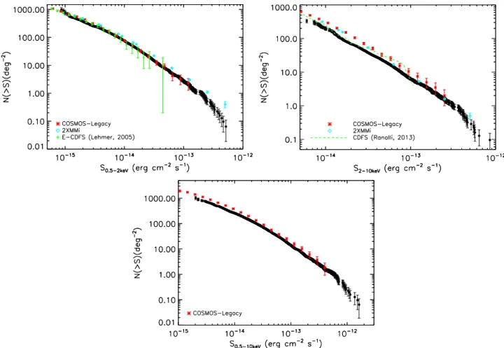
(6) The Astrophysical Journal, 817:172 (21pp), 2016 February 1. LaMassa et al. Table 3 X-ray Source Summarya Hardb. Fullc. Total. 969 1438 635 2440. 248 432 175 715. 1137 1411 668 2597. 1146 1607 751 2862. 5150. 1520. 5628. 6181. Survey. Soft. Archival Chandra (7.4 deg2) Archival XMM-Newton (6.0 deg2) XMM-Newton AO10 (4.6 deg2) XMM-Newton AO13 (15.6 deg2) Total (31.3 deg2)d. Notes. a The numbers correspond to the significant detections in each band. For Chandra, this is a 4.5σ level based on comparing the flux with the sensitivity map (see LaMassa et al. 2013b, for details) and for the XMM-Newton surveys, the det_ml has to exceed 15. b The hard band spans 2–10 keV for the XMM-Newton surveys but corresponds to 2–7 keV for the Chandra survey. c The broad band is 0.5–10 keV for the XMM-Newton surveys but ranges from 0.5–7 keV for the Chandra survey. d Duplicate observations of the same source and overlapping observations between surveys removed in total numbers.. 2015) in all three bands; and the wide-area 2XMMi Serendipitous Survey in the soft and hard bands (132 deg2; Mateos et al. 2008). The Stripe 82X Log N–Log S agrees with the reported trends from other surveys in the soft-band, the high-flux end in the hard and full bands, and with CDFS at the low-flux end (<2 ´ 10-14 erg s−1) in the hard band; discrepancies in these bands at lower fluxes (and between CDFS and COSMOS-Legacy and 2XMMi in the hard band at low fluxes) may be due to different methods for estimating survey sensitivity when generating area-flux curves and different assumed values for the power-law slope (Γ) when converting count rate to flux, and are not necessarily atypical when comparing number counts from different surveys. 4. MULTI-WAVELENGTH CATALOG MATCHING We searched for counterparts to the XMM-Newton AO13 sources in publicly available multi-wavelength databases: SDSS, WISE (Wright et al. 2010), UKIDSS (Hewett et al. 2006; Casali et al. 2007; Lawrence et al. 2007), VHS (McMahon et al. 2013), GALEX (Morrissey et al. 2007), FIRST, and the Herschel Survey of Stripe 82 (HerS; Viero et al. 2014). To determine whether a multi-wavelength association to an X-ray source represents the true astrophysical counterpart rather than a chance coincidence, we use the maximum likelihood estimator method (MLE; Sutherland & Saunders 1992) to match between the X-ray source lists and the ancillary catalogs. MLE takes into account the distance between an X-ray source and ancillary objects within the search radius, the astrometric errors of the X-ray and ancillary sources, and the magnitude distribution of ancillary sources in the background to determine whether a potential multi-wavelength counterpart is more likely to be a background source or a true match. This method has been implemented in many X-ray surveys to identify reliable counterparts (e.g., Brusa et al. 2007, 2010; Cardamone et al. 2008; Laird et al. 2009; Luo et al. 2010; Civano et al. 2012; LaMassa et al. 2013a; Marchesi et al. 2015). Ancillary objects within the search radius (rsearch ), which is set at 7″ for the XMM-Newton AO13 sources (see Brusa et al. 2010; LaMassa et al. 2013a), are assigned a likelihood ratio (LR), which is the probability that the correct counterpart. Figure 2. Area-flux curves for Stripe 82X in the soft (top), hard (middle), and full bands (bottom). While the colored curves show the full area for the individual data sets as indicated in the legends, the black curve illustrates the total area after removing observations from the archival Chandra and archival XMM-Newton surveys that overlap pointings from the XMM-Newton AO10 and/or AO13 surveys, and, in the case of the archival Chandra observations, archival XMM-Newton surveys; here, we have given preference to the widerarea coverage from XMM-Newton in overlapping pointings. Hence, deeper fluxes accessible by Chandra are consequently removed from the total Stripe 82X area-flux relation. The kink in the total area-flux curve in the hard and full bands comes from discontinuties induced by combining the individual areaflux curves from the archival pointings at lower flux limits.. soft band (0.3 deg2; Lehmer et al. 2005) and the XMM-Newton survey of CDFS in the hard band (∼0.25 deg2; Ranalli et al. 2013); the moderate-area, moderate-depth Chandra COSMOSLegacy Survey (2.2 deg2; Civano et al. 2015; Marchesi et al. 6.

(7) The Astrophysical Journal, 817:172 (21pp), 2016 February 1. LaMassa et al.. Figure 3. Cumulative Log N–Log S relationship for the Stripe 82X survey (black circles) in the soft (top left), hard (top right) , and full (bottom) bands. For reference, we also plot the source number density for other surveys, spanning the gamut from deep, pencil-beam surveys (i.e., the 0.3 deg2 ECDF-S and ∼0.25 deg2 CDFS; Lehmer et al. 2005; Ranalli et al. 2013, respectively), to a moderate-area, moderate depth survey (the 2.2 deg2 Chandra COSMOS-Legacy; Civano et al. 2015; Marchesi et al. 2015), and a wide-area survey (the 132 deg2 2XMMi Serendipitous Survey; Mateos et al. 2008).. is found within rsearch divided by the probability that a background ancillary source is there by chance: LR =. q (m ) f (r ) . n (m ). their positional errors underestimated by emldetect, such that counterparts were missed by the matching algorithm even though visual inspection of the X-ray sources and ancillary objects revealed bright multi-wavelength objects that are likely true matches (see also Brusa et al. 2010). Adding the 1″ systematic error recovered these associations. Accordingly, the archival XMM-Newton and AO10 catalogs published previously have been updated here. From LR, a reliability value is then calculated for every source:. (1 ). Here, q(m) is the expected normalized magnitude distribution of counterparts within rsearch which is estimated by subtracting the histogram of sources found within the search radius from the histogram of background objects, where each histogram is normalized by the relevant search areas; f(r) is the probability distribution of the astrometric errors23; and n(m) is the normalized magnitude distribution of sources in the background. The background sources are taken as the objects found in an annulus around each X-ray source with an inner radius of 10″ and an outer radius of 45″; thus, sources that are potential counterparts, i.e., within rsearch, are removed from the background estimation (Brusa et al. 2007). We note that the positional error for the X-ray sources includes a 1″ systematic error added in quadrature to the emldetect reported positional error to account for the lack of an external astrometric correction. This systematic astrometric error was not included in the previous release of the Stripe 82X catalog, and we subsequently found that bright X-ray sources tended to have. R=. LR , Si (LR)i + ( 1 - Q ). (2 ). where Q is the ratio of the number of X-ray sources that have ancillary objects within the search radius divided by the total number of X-ray sources; the LR sum is over every potential counterpart within the search radius of the X-ray source. This calculation is performed independently for every waveband to which we match the X-ray source list. We use R as a way to distinguish between true counterparts and chance associations. For X-ray sources that have more than one possible association within rsearch, we retain the potential counterpart with the highest reliability. To determine the critical reliability threshold above which we consider an association the true counterpart (Rcrit ), we followed the methodology in LaMassa et al. (2013a):. 23 f(r) is modeled as a two-dimensional Gaussian distribution where the X-ray and ancillary positional errors are added in quadrature.. 7.

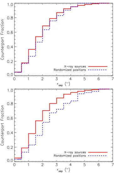
(8) The Astrophysical Journal, 817:172 (21pp), 2016 February 1. LaMassa et al.. we produced a catalog where we shifted the X-ray positions by random amounts and matched the multi-wavelength catalogs to these randomized positions. The resulting reliability distribution then gives us an estimate of the number of contaminating spurious associations above Rcrit. We pick our Rcrit threshold by examining the reliability histograms of the “true” matches, i.e., the original X-ray catalog, and the “spurious” matches, i.e., the catalog with randomized positions, in bins of 0.05 to determine where the fraction of spurious matches is ∼10%. That bin then becomes our threshold Rcrit value. As always, matching the X-ray source lists to ancillary catalogs is a balancing act between minimizing contamination from unassociated sources and maximizing counterpart identification. It is unavoidable that some true counterparts will be missed and that spurious associations will be promoted as real matches. In Sections 4.2–4.7 below, we note the number of spurious matches, i.e., the number of X-ray sources with randomized positions meeting the Rcrit threshold, to the number of total matches from the original X-ray catalog above Rcrit to provide an estimate of the counterpart contamination. We also show in Figures 4–10 the cumulative distribution of counterpart and spurious association fraction as a function of rsep, the distance between the X-ray and counterpart coordinates, for objects exceeding Rcrit. We remind the reader, however, that in addition to the separation between the sources, the astrometric error on both the X-ray and counterpart coordinates, the magnitude of the potential counterpart, and magnitude distribution of background sources all contribute to the calculated reliability value reported in the published catalogs. As the X-ray sources represent a menagerie of astronomical objects (stars, galaxies, obscured AGNs, and unobscured AGNs) they will have a range of spectral energy distributions and thus not have the same relative strength among all the wave-bands in each ancillary catalog. For example, heavily obscured AGNs are much brighter in the redder optical and infrared bands, and would have optical magnitudes in the bluer bands more consistent with background sources, or perhaps even be dropouts in these bands, while the converse is true for unobscured AGNs. We therefore match the X-ray source list separately to each band in the multi-wavelength catalogs, determine Rcrit independently for each passband, and then merge the individual lists where we report the maximum Rcrit values among the matches for that catalog. The only exception to this procedure for the MLE matching is WISE since the W1 band is the most sensitive filter; all WISE sources in Stripe 82 have detections in the W1 band so we do not miss any objects by matching to W1 only. A high level summary of the multiwavelength matches to the XMM-Newton AO 13 data is presented in the fifth column of Table 4.. Figure 4. Cumulative distribution of the fraction of X-ray sources with an rband counterpart above Rcrit as a function of distance between the X-ray and SDSS positions (rsep; red solid line) and between the randomized X-ray positions and SDSS sources (blue dashed line). The top panels are for the matches from single-epoch imaging (1852 X-ray/SDSS counterparts and 41 random matches) while the bottom panels show the matches to the coadded Jiang et al. (2014) catalog (1652 X-ray/coadded counterparts with 61 spurious associations). The number of spurious matches occurs at rsep distances similar to that as the un-shifted X-ray catalog, indicating that MLE helps to mitigate unassociated sources compared to nearest neighbor matching by using magnitude and astrometric precision information in the calculation.. catalog and not another, we promote that counterpart as a match in the latter catalog. To keep track of such promoted matches, we have included the following flags: “ch_cp_flag,” “xmm_archive_cp_flag,” and “xmm_ao13_cp_flag” to indicate which counterparts were promoted into that catalog based on MLE matching from the archival Chandra catalog, archival and AO10 XMM-Newton catalog, and AO13 XMM-Newton catalog, respectively. If these fields are empty, then the independent MLE matching to the individual catalogs gave consistent results. Otherwise, the following numbers indicate which multi-wavelength counterpart is the promoted match: 1 —SDSS counterpart found but photometry rejected for failing quality control checks; 2—SDSS; 3—redshift; 4—WISE counterpart found but rejected for failing quality control checks; 5—WISE; 6—UKIDSS; 7—VHS; 8—GALEX.24. 4.1. Cross-matches between X-Ray Catalogs For the X-ray sources that are repeated among the individual catalogs (archival Chandra, archival and AO10 XMM-Newton, and AO13 XMM-Newton catalogs), we checked their multiwavelength counterpart matches against each other. In most cases, these are consistent, but in some instances, a counterpart is not found for an X-ray source in one catalog yet is in another. This situation can arise due to differences in X-ray positions and positional errors between the individual sources lists, as well as the differences in the magnitude distribution of background sources. If a counterpart is found in one X-ray. 24. None of the UKIDSS or VHS matches were rejected for compromised photometry.. 8.

(9) The Astrophysical Journal, 817:172 (21pp), 2016 February 1. LaMassa et al.. Figure 5. Similar to Figure 4, but for the X-ray/WISE matches to the W1 band, where 2087 counterparts (seven spurious associations) are found (before discarding those failing quality control checks) above Rcrit.. Figure 8. Similar to Figure 4, but for the X-ray/GALEX matches to the NUV band, where 572 counterpartsand 12 matches to randomized positions lie above Rcrit.. Figure 9. Similar to Figure 4, but for the X-ray and FIRST nearest-neighbor matches, with 116 counterparts and eight randomized matches found within rsearch=7″. Here, many of the spurious associations are found at higher separation distances due to the low number density of radio and X-ray sources.. Figure 6. Similar to Figure 4, but for the X-ray/UKIDSS matches to the K band, where 1314 counterparts and 17 matches to randomized positions are found above Rcrit.. Figure 10. Similar to Figure 4, but for the X-ray and Herschel nearest-neighbor matches, with 121 counterparts and 8 spurious associations within rsearch=5″. Just as Figure 9 shows, the matching between the X-ray source list and FIRST, most of the spurious matches occurs at higher values of rsep.. Figure 7. Similar to Figure 4, but for the X-ray/VHS matches to the K band, where 1763 counterparts and 41 spurious associations are above Rcrit.. 9.

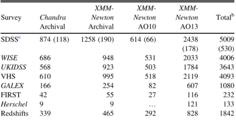
(10) The Astrophysical Journal, 817:172 (21pp), 2016 February 1. LaMassa et al.. meet these requirements are flagged in the “SDSS_rej” column as “yes” in the catalog, though we retain the SDSS coordinates and ObjID to note that these sources are optically detected even if the photometry is compromised. Finally, we check the remaining images by eye to remove optical artifacts, such as diffraction spikes and noise due to emission from nearby bright objects. We then matched the full X-ray catalog to the coadded SDSS source lists presented in Jiang et al. (2014), which are 1.9–2.2 mag deeper than the single-epoch SDSS imaging, with 5σ magnitude limits of 23.9, 25.1, 24.6, 24.1, and 22.8 (AB) in the u, g, r, i, and z bands. Here, we utilize the mag_auto fields returned by SExtractor (Bertin & Arnouts 1996) for the MLE algorithm. Jiang et al. (2014) performed the image coaddition by separating each of the 12 SDSS parallel scans that cover Stripe 82 into 401 individual regions, extracting aperture magnitudes separately for each of the five bands. They then provide 24,060 individual catalogs, where each band, region, and scan line are independent catalogs, which can include duplicate observations of the same source among these catalogs that cover adjacent area. Thus, we first produced “cleaned” SDSS coadded catalogs by only retaining objects within 45″ of the XMM-Newton AO13 sources, since these are the data we need to estimate the background and find counterparts. We then search for duplicate observations within each band by searching for matches within 0 5, retaining the coordinates and photometry for the object that has the highest signal-tonoise. We match the X-ray sources to each of these cleaned coadded catalogs. Here, the astrometric errors in the coadded images are similar to those of the single-epoch images due to the method used when generating the coadds (Jiang et al. 2014). However, we conservatively used a value of 0 2 based on observed positional offsets between SDSS coadded sources and FIRST objects (I. McGreer 2015, private communication). We find the following Rcrit cut-offs: u— 0.85, g—0.9, r—0.9, i—0.9, z—0.85, with the spurious association rate being 20/1799, 41/1751, 61/1652, 40/1530, and 37/1816, respectively; the cumulative fraction of matches as a function of rsearch above Rcrit for both the X-ray source list and randomized positions is shown in the bottom panel of Figure 4. We note that the lower number of sources here compared with the single-epoch imaging data is due to the higher reliability thresholds we impose for the coadded catalog. However, the number of spurious associations in the lower reliability bins becomes a much higher fraction of the total number of true X-ray sources in those bins, so we have erred on the side of caution to minimize the number of random associations in our sample. From these counterparts found from matching to the coadded images, we keep only the sources that do not have a counterpart in the single-epoch imaging. Since Jiang et al. (2014) do not provide a band-matched catalog or cross-identify the same source among the multiple-bands, we consider an optical source to be the same object if it is within ∼0 6 with no other object found in that band within 1″; if no match in another band is found meeting these requirements, the source is assumed to be a drop-out in that band. The reported SDSS coordinates are the average of the coordinates in the individual band catalogs where the source is detected. The objects found from the coadded catalog are marked in the “SDSS_coadd” column as “yes.”. Table 4 Multi-wavelength Counterpart Summarya Survey. Chandra Archival. SDSSc. 874 (118). WISE UKIDSS VHS GALEX FIRST Herschel Redshifts. 686 568 610 166 42 9 339. XMMNewton Archival. XMMNewton AO10. XMMNewton AO13. Totalb. 1258 (190). 614 (66). 948 923 995 254 55 9 465. 531 503 518 82 27 K 292. 2438 (178) 2033 1784 2119 607 116 121 828. 5009 (530) 4006 3643 4093 1080 232 133 1842. Notes. The counterpart numbers quoted in the text refer to associations found from matching the individual X-ray catalogs with the multi-wavelength source lists. Here, we include the final numbers that include “promoted” matches, found from cross-correlating the counterparts among the X-ray catalogs (see Sections 4.1 and A.7 for details). b Duplicate sources among surveys removed from total numbers. c Includes matches to the single-epoch and coadded catalogs. The number of sources found in the coadded catalog that do not have matches in the singleepoch data are quoted in parentheses. a. While the number of matches quoted in the text below refer to the sources above Rcrit in each catalog, the tally in the Table 4 include the promoted counterparts found from crossmatching the catalogs. The remainder of this section pertains to the multi-wavelength catalog matching to the XMM-Newton AO13 source list, while updates to the previous released Stripe 82X catalogs are discussed in the Appendix. 4.2. SDSS We matched the X-ray sources to the separate u, g, r, i, and z bands in the single-epoch SDSS photometry from Data Release 9 (Ahn et al. 2012, DR9), where a uniform 0 1 error was assumed for the SDSS astrometry (Rots & Budavári 2011). We imposed the following Rcrit values for the individual SDSS bands: u—0.75, g—0.80, r—0.85, i—0.85, z—0.80, with the estimated number of spurious association rate being 36/1989, 43/2006, 41/1852, 21/1819, and 51/1926, respectively. Figure 4 (top) shows the cumulative distribution of counterparts and spurious associations above the r-band Rcrit value as a function of distance between the X-ray and SDSS source. We removed from these individual band source lists any SDSS object that did not exceed the Rcrit threshold, and then checked by eye the instances where more than one SDSS source is matched to an X-ray source to determine which optical source is the most likely counterpart. The preferred match is usually the SDSS source with the greatest number of matches among the individual bands and/or the brightest object. From our band-merged list, we then perform a photometric quality control to check for saturation, blending, or photometry that is not well measured.25 Objects that do not 25. We report the photometry for objects that meet the follow requirements: (NOT_SATUR) OR (SATUR AND (NOT SATUR_CENTER)), (NOT BLENDED) OR (NOT NODEBLEND), (NOT BRIGHT) AND (NOT DEBLEND_TOO_MANY_PEAKS) AND (NOT PEAKCENTER) AND (NOT NOTCHECKED) AND (NOT NOPROFILE). An object that failed any of these quality control checks has the photometry set to -999 in the catalog.. 10.

(11) The Astrophysical Journal, 817:172 (21pp), 2016 February 1. LaMassa et al.. In total, we find SDSS counterparts for 2438 X-ray sources (85% of the sample), 178 of which are not found in the singleepoch SDSS imaging but are detected in the coadded catalog, and as expected are generally fainter. We list the information for the SDSS counterparts found from the single-epoch catalog, where available, to allow the user to easily query the main SDSS database to fetch relevant information using the unique SDSS ObjID or SDSS coordinates; similar data, such as aperture magnitudes and errors, from the coadded Jiang et al. (2014) catalog would involve querying 24,060 individual catalogs, while such data are linked in the main SDSS database.. When doing the MLE matching to the W1 band, using the “w1mpro” magnitude measured via profile-fitting photometry, we use a Rcrit of 0.9, with seven spurious associations out of 2087 matches (see Figure 5). We then impose photometry control checks on the WISE sources, following our prescription in LaMassa et al. (2013a). We null out the magnitude in any band that was saturated (i.e., the fraction of saturated pixels, “wnsat” exceeds 0.05, where n refers to the band number); is likely a spurious detection associated with artifacts such as diffraction spikes, persistence, scattered light from nearby bright sources (i.e., if the “cc_flag” is non-zero); or moon level contamination (i.e., if “moon_lev”  5, where “moon_lev” is the ratio of frames affected by scattered moonlight to the total number of frames and spans from 0 to 9). We also isolate extended sources, as their “wnmpro” magnitudes would be unreliable. These sources have the “ext_flag” set to non-zero. For these objects, we downloaded their elliptical photometry magnitudes (“wngmag”) and discarded their photometry if their extended photometry magnitude flags were non-null. If a matched WISE source has photometry that fails the point-like or extended photometry quality checks in all bands, then the “wise_rej” flag is set to “yes” in the catalog and the associated photometry and coordinates are not reported. Of the 2087 matched sources, 2031 (71% of the XMMNewton AO13 sources) passed the quality assurance tests above. All the rejected sources were extended. Ten extended sources had non-flagged elliptical magnitude measurements and are marked with the “wise_ext” flag set to “yes” in the catalog.. 4.2.1. Optical Spectra. We mined the following public spectroscopic catalogs to find redshifts, and where possible, optical classifications of the X-ray sources with SDSS counterparts: SDSS Data Release 12 (DR12; Alam et al. 2015), 2SLAQ (Croom et al. 2009), preBOSS pilot survey using Hectospec on MMT (Ross et al. 2012), and 6dF (Jones et al. 2004, 2009). We checked by eye the 41 spectra that had the zwarning flag set by the SDSS pipeline. While we were able to verify some of these redshifts, we were not able to find a reliable redshift solution for 26 of these objects, and consequently set their redshifts to zero in the catalog. We also obtained spectra for 12 and 6 sources in 2014 September and 2015 January, respectively, through our dedicated follow-up program with WIYN HYDRA; the spectra were reduced with the IRAF task dohydra where we identified redshifts based on emission and/or absorption features, or classified stars on the basis of their rest-frame absorption and emission lines. About 29% of the X-ray sources (828 objects) have secure redshifts. The calculation of photometric redshifts for the remainder of the sources is underway (T. Ananna et al. 2015, in preparation). The databases we mined provide an automatic classification of sources based on their optical spectra, where “QSO”s or “AGNs” are objects that have at least one broad emission line in their spectra (generally a full-width half max exceeding 2000 km s−1). Sources lacking broad emission lines are classified as “galaxies,” where this type includes objects with narrow emission lines (Type 2 and elusive AGNs, i.e. those objects with emission line ratios consistent with star-forming galaxies; Baldwin et al. 1981; Maiolino et al. 2003), absorption lines only, and even blazars with featureless optical spectra that are not flagged as active galaxies by optical spectroscopic pipelines. We have followed this methodology when classifying sources from our spectroscopic follow-up campaign, where we reserve the class QSO to refer to broad-line objects and galaxies for sources lacking broad-lines. Stars are identified by emission and absorption transitions in their optical spectra.. 4.4. Near-infrared The XMM-Newton AO13 source list was matched independently to the near-infrared (NIR) catalogs from the UKIDSS Large Area Survey (LAS; Hewett et al. 2006; Casali et al. 2007; Lawrence et al. 2007; Warren et al. 2007) and VHS (McMahon et al. 2013). From both catalogs, we chose primary objects from the database26 and eliminated objects that were consistent with noise, i.e., “mergedclass” set to zero and “pnoise”27 >0.05. The magnitudes presented in the catalog are the “apermag3” values from the UKIDSS LAS and VHS databases, which are aperture-corrected magnitudes, with a 2″ diameter aperture. We matched the XMM-Newton AO13 source list to Data Release 8 of the UKIDSS LAS survey. Matching separately to the Y (0.97–10.07 μm), J (1.17–1.33 μm), H (1.49–1.78 μm), and K (2.03–2.37 μm) bands, we find Rcrit values of 0.75, 0.85, 0.75, 0.75, respectively, with a spurious association rate of 21/1375, 15/1070, 18/1335, and 17/1314, respectively (see Figure 6). When merging the separate lists together, we find a total of 1784 near-infrared counterparts, or 62% of the X-ray sample. We performed quality control checks on the photometry as explained in LaMassa et al. (2013a) to check for saturation, but no objects were flagged as being possibly saturated. We used Data Release 3 of the VHS survey to match to the XMM-Newton AO13 catalog, where we adopt an astrometric uncertainty of 0 14 for the VHS sources. VHS has coverage over Stripe 82 in the J, H, and K bands, where we impose Rcrit values of 0.75 in each band, with a spurious counterpart rate of. 4.3. WISE Since publishing our initial Stripe 82X multi-wavelength matched catalogs in LaMassa et al. (2013a), the AllWISE Source Catalog was released, combining data from the cryogenic and NEOWISE missions (Wright et al. 2010; Mainzer et al. 2011). As this catalog has enhanced sensitivity and astrometric precision, we match the XMM-Newton AO13 X-ray source list to this release, and update the archival Chandra and XMM-Newton and XMM-Newton AO10 matches to AllWISE, as detailed in the appendix.. 26 27. 11. priOrSec=0 OR priOrSec=frameSetId. “Pnoise” is the probability that the detection is noise..

(12) The Astrophysical Journal, 817:172 (21pp), 2016 February 1. LaMassa et al.. 20/1856, 39/1783, and 41/1763, respectively (see Figure 7). In total, 2117 XMM-Newton AO13 sources (74% of the sample) have NIR counterparts from the VHS survey. We also check the “mergedClass” flag to test if a source is saturated (“mergedClass”=−9), but none of the matches are so afflicted. Between UKIDSS and VHS, we find NIR counterparts for 2257 X-ray sources, or 79% of the sample. Of the NIR sources, 140 are found in UKIDSS, but not VHS. Of these, 34 were non-detections in VHS (i.e., no match between VHS and UKIDSS within a 2″ search radius), while the remaining 106 were found in VHS but fell below our reliability thresholds for this catalog; we note that 77 of these VHS sources below the reliability cut had UKIDSS Y-band reliabilities above our Y-band critical threshold, while VHS is lacking this coverage. By presenting matches to both UKIDSS and VHS, the variability of the 1678 X-ray selected, NIR objects (1644 objects in common between UKIDSS and VHS and the 34 VHS dropouts) can be studied by the community.. Krolik 1992), making these data of particular importance to study the host galaxies of AGNs (Pier & Krolik 1992; Efstathiou & Rowan-Robinson 1995; Lutz et al. 2004; Fritz et al. 2006; Schweitzer et al. 2006; Netzer et al. 2007; Schartmann et al. 2008; Shao et al. 2010; Mullaney et al. 2011; Rosario et al. 2012; Magdis et al. 2013; Delvecchio et al. 2014). Indeed, the XMM-Newton AO13 survey was specifically designed to overlap existing Herschel coverage, since similar far-infrared data will not be available in the foreseeable future. Similar to the matching to the FIRST catalog, we employed a nearest neighbor approach to find associations between the farinfrared Herschel sources and the X-ray objects. However, we shortened rsearch to 5″ since our exercise of matching the Herschel catalog to the random X-ray positions reveals that most spurious associations occurred at distances between 5″ and 7″. We found 121 Herschel sources within 5″ of the XMMNewton sources, corresponding to 4% of the sample, and 8 spurious associations when matching to the randomized X-ray positions (see Figure 10).. 4.5. GALEX 4.8. XMM-Newton AO13 Multiwavelength Match Summary. Similar to the UKIDSS matching, we used the cleaned GALEX catalog described in LaMassa et al. (2013a) to find counterparts to the XMM-Newton AO13 sources, matching to the near-ultraviolet (NUV) and far-ultraviolet (FUV) bands independently. This catalog represents data from the mediumimaging survey (MIS) in GALEX Release 7 (Morrissey et al. 2007). With a Rcrit value of 0.75 for both bands, we find 572 and 407 counterparts, with 12 and 5 spurious associations, in the NUV and FUV bands, respectively (see Figure 8). In total, 607 X-ray sources have ultraviolet counterparts, corresponding to 21% of the XMM-Newton AO13 sample.. In total, we find counterparts to 93% of the XMM-Newton AO13 sources. However, we emphasize that we matched the X-ray source list independently to each of the multi-wavelength catalogs and did not cross-correlate the counterparts. In a vast majority of the cases, these counterparts among the catalogs are the same source, though discrepancies exist. For guidance, we include a “cp_coord_flag” to note which sources have counterparts with consistent coordinates and which do not, using a search radius of 2″ for SDSS, UKIDSS, VHS, and FIRST and 3″ for WISE, GALEX, and Herschel due to the larger PSF and higher astrometric uncertainties in these latter catalogs compared with the former. When the coordinates are inconsistent within these search radii, the “cp_coord_flag” is set to one; otherwise it is set to null. For 89% of the X-ray sources with counterparts, their coordinates are consistent. We note, however, that above these search radii, consistent counterparts may exist and below these radii, there can still be discrepencies. Finally, we highlight that the multi-wavelength magnitudes in the Stripe 82X catalogs may not be the most appropriate magnitude for every source and it is up to the user to determine whether different aperture photometry should be downloaded from the original catalog, using the identifying information presented in our catalogs to isolate the correct source, for the intended science goals. A summary of the multi-wavelength columns and flags is presented in the appendix, as well as a discussion of updates made to the previously released Stripe 82X catalogs.. 4.6. FIRST Due to the relatively low space density of the radio sources detected in the FIRST (Becker et al. 1995; White et al. 1997) survey, we used a nearest neighbor match to find counterparts to the X-ray sources, using the same search radius of 7″ as employed in the MLE matching above. Similar to our previous Stripe 82X catalog release, we used the FIRST catalog published in 2012 which includes all sources detected between 1993 and 2011, which has a 0.75 mJy flux limit over the XMMNewton AO13 region (Becker et al. 2012). Since our previous paper, the final FIRST catalog has been published (Helfand et al. 2015) but we do not gain any additional sources when matching to this final catalog, both with the XMM-Newton AO13 data and archival Chandra and archival and AO10 XMM-Newton catalogs. Of the X-ray sample, 116 FIRST sources (4% of the X-ray sample) are found within 7″ of the XMM-Newton AO13 sources. When matching the FIRST catalog to the randomly shifted X-ray positions, eight spurious associations were found (see Figure 9).. 5. DISCUSSION When considering the full Stripe 82X survey to date, including archival Chandra, archival XMM-Newton, XMMNewton AO10, and XMM-Newton AO13 data, we find multiwavelength counterparts to 88% of the X-ray sources. We are able to identify ∼30% of the Stripe 82X sample with spectroscopic objects. Of the sample, 67 objects are classified as stars while the remaining 1775 objects are extragalactic. We plot the r-band magnitude as a function of soft X-ray flux for all objects with optical counterparts in Figure 11, where we. 4.7. Herschel The Herschel Stripe 82 Survey (HerS) covers 79 deg2 at 250, 350, and 500 μm to an average depth of 13.0, 12.9, and 14.8 mJy beam−1 at >3σ, surveyed with the Spectral and Photometric Imaging Receiver (SPIRE) instrument (Viero et al. 2014). The far-infrared emission from Herschel provides a clean tracer of host galaxy star-formation (Pier & 12.

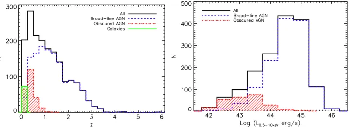
(13) The Astrophysical Journal, 817:172 (21pp), 2016 February 1. LaMassa et al.. Figure 11. SDSS r-band magnitude as a function of observed X-ray flux in the 0.5–2 keV band. The solid line defines the typical X-ray-to-optical flux ratio of AGNs (Brandt & Hasinger 2005), while the dashed lines show the X/O=±1 locus within which most AGNs lie (see Equation (3)). Stars are identified by their optical spectra while AGNs and galaxies are classified based on their observed 0.5–10 keV luminosity, with 1042 erg s−1 being the dividing line.. Figure 12. r - W1 (AB) color as a function of r − K (AB) color for the 1891 X-ray sources with SDSS, UKIDSS, and WISE counterparts that have K-band and W1 detections and UKIDSS (WISE) coordinates within 2″ (3 ) of the SDSS position. Many of the stars can be identified by the distinct track they occupy in this color space (LaMassa et al. 2015b).. note which objects are stars, X-ray AGNs, X-ray galaxies, and currently unidentified (i.e., they lack redshifts). Stars are classified on the basis of their optical spectra while here we use the observed, full-band X-ray luminosity to differentiate between X-ray AGNs (L 0.5 - 10 keV > 10 42 erg s−1) and X-ray galaxies (L 0.5 - 10 keV < 10 42 erg s−1), independent of their optical spectroscopic classification. For reference, we also include lines to mark typical AGNs X/O values (e.g., Brandt & Hasinger 2005):. X-ray surveys in the absence of supporting spectroscopic information.. X/O = Log (fx fopt ) = log (fx ) + C + 0.4 ´ m r ,. 5.2. Extragalactic Objects In Figure 13 (left), we show the redshift distribution of the 1775 extragalactic sources with optical spectra: about half (875) are at z>1, with 301 at redshifts above 2. We further break down the redshift distribution by classification, based on optical spectroscopy (see Section 4.2.1) and X-ray luminosity. In Figure 13, “broad-line” AGNs are sources optically classified as quasars due to broad emission lines in their spectra, “obscured AGNs” are sources optically classified as galaxies whose full-band observed X-ray luminosities exceed 1042 erg s−1, and “galaxies” are objects lacking broad-lines in their optical spectra whose X-ray luminosities are below 1042 erg s−1; we note, however, that this “galaxy” class can include Compton-thick AGNs (NH > 1.25 ´ 10 24 cm−2) with very weak observed X-ray emission due to heavy attenuation. Of the 1775 extragalactic sources in our sample, 19 are not classified in the spectroscopic databases we utilized and another 30 do not have significant detections in the full X-ray band. The left-hand panel of Figure 13 demonstrates that nearly all the sources we have identified thus far at high redshifts (i.e., z>1) are broad-line AGNs, in part because unobscured quasars were preferentially selected as spectroscopic targets in the SDSS surveys. Most of the obscured AGNs live within the intermediate universe (z∼0.5) while galaxies reside in the local universe (z<0.25). We expect the percentage of obscured AGNs, i.e., those lacking broad emission lines, to increase as more objects are identified via spectroscopic and photometric redshifts. In the right-hand panel of Figure 13, we show the observed full-band luminosity distribution of the X-ray AGNs, 1603 sources in total. The distribution peaks at relatively high luminosities (∼44.5 dex) due to the wide-area and shallow design of the survey. Most of the high luminosity AGNs are broad-line sources, though a handful of obscured AGNs do. (3 ). where C is a constant based on the optical filter, which for the SDSS r-band, is 5.67 (see Green et al. 2004). Previous studies have found that AGNs generally fall within the X/0=0±1 locus (e.g., Schmidt et al. 1998; Alexander et al. 2001; Green et al. 2004; Brusa et al. 2007; Xue et al. 2011; Civano et al. 2012), as indicated by the dashed lines in Figure 11. We find the same trend here, and note that extragalactic objects do not separate out from Galactic objects within this color space. 5.1. Stars In Figure 12, we show how most X-ray emitting stars can be cleanly identified on the basis of their optical and infrared properties by comparing their r - K and r - W1 colors, as presented in LaMassa et al. (2015b). Here, we focus on the X-ray sources with SDSS, UKIDSS, and WISE counterparts that have K-band detections, W1 detections (W1 SNR >2), and an r-band magnitude under 22.2 (the 95% completeness limit for the single-epoch SDSS imaging catalog) to avoid artificially inflating the colors to redder values. Additionally, we only retain the sources where the SDSS and UKIDSS coordinates are consistent within 2″ and the SDSS and WISE coordinates agree within 3″ to minimize spurious associations. In total, 1891 objects are shown in Figure 12, compared with the 4133 sources shown in the previous plot, which are sources detected in the r and soft X-ray bands. Most of the stars follow a welldefined track in r - K versus r - W1 color space, aiding in the separation of Galactic and extragalactic candidates detected in 13.

(14) The Astrophysical Journal, 817:172 (21pp), 2016 February 1. LaMassa et al.. Figure 13. Left: spectroscopic redshift distribution of the 1775 extragalactic Stripe 82X sources, with different classes of objects highlighted. Half the sample is above a redshift of one, and contains predominantly broad-line AGNs at these distances. Nearly all obscured AGNs (i.e., sources optically classified as galaxies with but with full band X-ray luminosities above 1042 erg s−1) are at a redshift below 1, while the optical and X-ray galaxies are at z<0.25 (Compton-thick AGNs that have low observed X-ray flux due to heavy obscuration can be included in the “galaxy” bin). Right: observed full-band luminosity distribution for the 1603 spectroscopically confirmed X-ray AGNs (i.e., L 0.5 - 10 keV > 10 42 erg s−1), where the distribution peaks at high-luminosities (44.25 dex < Log(L 0.5 - 10 keV erg s−1) < 45.25 dex). Highluminosity AGNs are predominantly broad-line sources while the lower-luminosity AGNs are mostly obscured. We note that these trends are for the ∼30% of the parent Stripe 82X sample that have spectroscopic redshifts and that with increased completeness and more sources identified via photometric redshifts, we expect to confirm more AGNs at all luminosities and redshifts, including at z>2 and L 0.5 - 10 keV > 10 45 erg s−1, and a higher percentage of obscured AGN.. Figure 14. Left: K-corrected (rest-frame) soft-band (0.5–2 keV) luminosities as a function of redshift for the Stripe 82X (red diamonds), COSMOS-Legacy (blue asterisks; Civano et al. 2015; Marchesi et al. 2015), and CDFS (black crosses) sources. At every redshift, an increase in survey area preferentially identifies higherluminosity sources. Right: normalized distribution of k-corrected soft-band luminosities for Stripe 82X compared with COSMOS and CDFS: the wide-area coverage of Stripe 82X which probes a large effective volume of the universe, enables the rare, highest luminosity quasars to be uncovered, complementing the parameter space explored by small- to moderate-area surveys. In both plots, only the sources identified with redshifts are plotted, representing 30% of the Stripe 82X sample (which currently has only spectroscopic redshifts) and 91% and 96% of the CDFS and COSMOS-Legacy sample, respectively, where both spectroscopic and photometric redshifts are available.. reach moderately high X-ray luminosities (Log (L 0.5 - 10 keV /erg s−1) > 43.75 dex).. become shallower, the detected sources are preferentially at higher luminosity at every redshift. This is further illustrated in Figure 14 (right), which compares the normalized luminosity distribution of Stripe 82X with COSMOS and CDFS, highlighting the complementarity of the different survey strategies in preferentially identifying sources within different luminosity ranges (see, e.g., Hsu et al. 2014). Wide-area surveys which explore a large volume of the universe, like Stripe 82X, are necessary to discover rare objects that have a low space density, including the highest luminosity quasars. One important caveat in Figure 14 is that we limit our comparison to sources with measured redshifts. For Stripe 82X, this represents the 30% of the sample that has spectroscopic redshifts while COSMOS and CDFS have spectroscopic and photometric redshifts, effectively identifying ∼96% and ∼91%. 5.3. The L – z Plane Probed by Stripe 82X To put the Stripe 82X sample in context with other surveys, we compare the luminosity-redshift plane with the small-area, deep CDFS survey (0.13 deg2; Xue et al. 2011) and the moderate-area, moderate-depth COSMOS-Legacy survey (2.2 deg2; Civano et al. 2015; Marchesi et al. 2015). Here, we use soft-band (0.5–2 keV) luminosities that have been kcorrected to the rest-frame, using Γ=1.4 for CDFS and COSMOS, while no k-correction was needed for Stripe 82X as the soft-band flux was estimated using Γ=2 and the kcorrection scales as (1 + z )(G- 2). As Figure 14 (left) shows, as survey area increases and the effective flux limits of the surveys 14.