New interactions in a mammalian community : introduced lagomorphs sustain native carnivores in the Andes of central Chile

Texto completo

(1)PONTIFICIA UNIVERSIDAD CATOLICA DE CHILE FACULTAD DE AGRONOMIA E INGENIERIA FORESTAL DIRECCION DE INVESTIGACION Y POSTGRADO MAGISTER EN RECURSOS NATURALES. NEW INTERACTIONS IN A MAMMALIAN COMMUNITY: INTRODUCED LAGOMORPHS SUSTAIN NATIVE CARNIVORES IN THE ANDES OF CENTRAL CHILE. Thesis presented as requisite to obtain the degree of Magíster en Recursos Naturales by:. José Domingo Infante Varela. Thesis Committee Supervisor: Cristián Bonacic Informant Professors: José Tomás Ibarra Nicolás Gálvez. June 2019 Santiago-Chile.

(2) ACKNOWLEDGEMENTS. This thesis would not have been possible without the economical and logistical support from Pacific Hydro Chile, who financed fieldworks and materials through the “Fondo Científico del Alto Cachapoal, Versión VI”. Rodrigo Órdenes and Zandra Monreal from Pacific Hydro were substantial part of it. Thank you. People who gave their support, either intellectual, economical, technical, emotional, or physical, were an invaluable piece of this work, and I will always owe them special gratitude. I would like to thank my family, specially my parents, Susana and Pedro, whose support, patience and encouragement were fundamental to fulfilling this goal. Also, I thank all my brothers and sisters, who constantly encouraged me to follow this new path. I want to thank National Forest Service (CONAF)-VI Region, and park rangers and the administrator from Río de los Cipreses National Reserve, who supported my entry and work inside the study area, and let me take part of the incredible experience of guanaco census inside the reserve. I sincerely thank all my field colleagues, assistants and friends from Fauna Australis Wildlife Laboratory, who altruistically worked many days for this research, enduring long fieldwork journeys or in laboratory analyses: Franco Perona, Fernando Novoa, Rocío Almuna, José Blanco, Ana Muñoz and Valentina Undurraga. I also thank other friends who contributed on fieldwork labors: Jaime Marmolejo, Jerry Laker, Enrique “Quico” Lara and Ángel Lara father and son. I also want to thank my thesis advisor, Cristián Bonacic, who trusted in my capabilities from the beginning of this work, even with little or no experience on wildlife research, and to whom I owe most of what I have learned all these years. I also thank the rest of my thesis committee: Tomás Ibarra and Nicolás Gálvez, whose corrections and comments on the final versions of this thesis were fundamental. Finally, thank you Beatriz, for your daily emotional support, encouragement, patience, and love, that kept me working for achieving this goal..

(3) To my mother, father, and Beatriz, To nature and its secrets.

(4) INDEX. ABSTRACT ....................................................................................................................................... 8 INTRODUCTION .............................................................................................................................. 9 Hypothesis ................................................................................................................................. 13 Objectives................................................................................................................................... 13 METHODS ....................................................................................................................................... 14 1.. Study area ................................................................................................................ 14. 2.. Field surveys ..................................................................................................................... 16. Assessing the diet of native carnivores ............................................................................. 16 Camera trap survey design.................................................................................................... 17 3.. Data analyses .................................................................................................................... 18. Daily activity pattern overlaps .............................................................................................. 18 Hierarchical modelling ............................................................................................................ 18 RESULTS ........................................................................................................................................ 27 Diet of native carnivores ........................................................................................................ 27 Camera trap general results .................................................................................................. 30 Daily activity pattern overlaps .............................................................................................. 30 Models results ........................................................................................................................... 33 Guanaco.................................................................................................................................. 33 Hare .......................................................................................................................................... 33 Rabbit ...................................................................................................................................... 34 Culpeo Fox ............................................................................................................................. 34 Puma ........................................................................................................................................ 35 Summary figures ...................................................................................................................... 36 DISCUSSION .................................................................................................................................. 38 RESUMEN ....................................................................................................................................... 64 REFERENCES ............................................................................................................................... 66 APPENDICES ................................................................................................................................. 76. 1.

(5) LIST OF FIGURES. Figure 1. Study area. Left map shows the location of the Libertador Gral. Bernardo O’Higgins Region (green area) in central Chile (blue area). Right map shows the 3.7 x 3.7 km grid of sites and camera trap locations from 2013, 2015 and 2017 surveys inside the study area ........................................................................................................................................ 15. Figure 2. Modelling approach used to asess species interactions. A) Data used for modelling prey species parameters. Layers on the left represent environmental features in the study area (vegetation, climatic and topographic variables), right camera symbol represent photos of prey species; B) data used for modelling predator species parameters of occupancy/abundance, colonization/recruitment and extinction/apparent survival, depending on the type of model applyied. Left map represents predicted distribution and abundance of prey species, right camera symbol represents photographic captures of the predator species; C) Relevant interactions driving predators’ parameters detected by best models. ............................................................................................................................................. 20. Figure 3. Activity pattern overlaps between puma (P. concolor) and its preys: A. guanaco (L. guanicoe), B. hare (L. europaeus), C. rabbit (O. cuniculus), D. rodents, E. livestock and F. culpeo fox (L. culpaeus); in autumn-winter seasons in Río los Cipreses National Reserve, Central Chile, years 2013-2017. The y-axis shows kernel density estimation and x-axis shows time of day. Black line and dashed line represent species activity pattern being compared. Grey area represents activity overlap between both species being compared, and Δ corresponds to kernel index of overlap, showing 95% compatibility intervals inside parenthesis. ..................................................................................................................................... 31. Figure 4. Activity pattern overlaps between hares (L. europaeus) and guanacos (A,) and between fox (L. culpaeus) and its preys: B. hare (L. europaeus), C. rabbit (O. cuniculus), and D. small mammals, in autumn-winter seasons in Río los Cipreses National Reserve, Central Chile, years 2013-2017. The y-axis shows kernel density estimation and x-axis shows time of day. Black line and dashed line represent species activity pattern being compared. Grey area represents activity overlap between both species being compared, and Δ corresponds to kernel index of overlap, showing 95% compatibility intervals inside parenthesis. ..................................................................................................................................... 32 2.

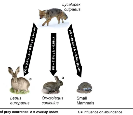
(6) Figure 5. Summary of fox (L. culpaeus) interactions with native and introduced mammal preys occurring inside the study area. Percentage of prey occurrence in fox diet (PO), kernel density estimation (Δ), and state variables (λ, γ, and ω) influenced by prey abundances are displayed. We show state variables in the interaction arrow only when there is influence of the prey abundance patterns in the best model or in alternative models (indicated by a “c”), with p-value below or around 0.05. .............................................................................................. 36. Figure 6. Summary of puma (P. concolor) interactions with native and introduced mammal species occurring inside the study area. Percentage of prey occurrence in puma diet (PO), kernel density estimation (Δ), and state variables (Ψ, γ, and ε) influenced by prey abundances are displayed. We show state variables in the interaction arrow only when there is influence of the prey abundance patterns in the best model or in alternative models (indicated by a “c”), with p-value below or around 0.05............................................................ 37. Figure 7. Guanaco (L. guanicoe) group abundance predictions from best models for each site and season (months) in the study area. Scale of grey represents relative abundance predicted from less abundant (white colored sites) to most abundant (black colored sites). Compatibility intervals of predictions are shown in parenthesis.............................................. 53 Figure 8. Hare (L. europaeus) best model’s abundance predictions for each site and season (months) in the study area. Scale of grey represents relative abundance predicted from less abundant (white colored sites) to most abundant (black colored sites). Compatibility intervals of predictions are shown in parenthesis. .................................................................................... 54 Figure 9. Rabbit (O. cuniculus) best model’s abundance predictions for each site and season (months) in the study area. Scale of grey represents relative abundance predicted from less abundant (white colored sites) to most abundant (black colored sites). Compatibility intervals of predictions are shown in parenthesis.............................................. 55 Figure 10. Fox (L. culpaeus) best model’s relative abundance predictions for each site and season (months) in the study area. Scale of grey represents relative abundance predicted from less abundant (white colored sites) to most abundant (black colored sites). Compatibility intervals of predictions are shown in parenthesis.............................................. 56 3.

(7) Figure 11. Puma (P. concolor) best model’s occupancy probability predictions for each site and season (months) in the study area. Scale of grey represents occupancy probability predicted from less probable (white colored sites) to most probable (black colored sites). 57 Figure 12. Best models’ detection probability response to selected covariates for open population of prey species, Río Los Cipreses National Reserve and Verde Valle & Los Coligües, Libertador General Bernardo O’Higgins Region, 2013-2017. Grey area shows 95% compatibility intervals. ........................................................................................................... 58 Figure 13. Best models’ recruitment probability response to selected covariates for open population of prey species, Río Los Cipreses National Reserve and Verde Valle & Los Coligües, Libertador General Bernardo O’Higgins Region, 2013-2017. Grey area shows 95% compatibility intervals. ........................................................................................................... 59 Figure 14. Best models’ relative abundance response to selected covariates for open population of prey species, Río Los Cipreses National Reserve and Verde Valle & Los Coligües, Libertador General Bernardo O’Higgins Region, 2013-2017. Grey area or whiskers shows 95% compatibility intervals............................................................................... 60 Figure 15. Best models’ detection probability (upper graphics) and recruitment probability (lower graphics) response to selected covariates for open population of predator species, Río Los Cipreses National Reserve and Verde Valle & Los Coligües, Libertador General Bernardo O’Higgins Region, 2013-2017. Grey area or whiskers shows 95% compatibility intervals. X axis of upper-right graph shows the four observers involved in camera surveys: Nicolás Guarda (NG), Ana Muñoz (AM), José Infante (JI), and Conaf (CN). ....................... 61 Figure 16. Best models’ apparent survival (upper graphics) and extinction probability (lower graphic) response to selected covariates for open population of predator species, Río Los Cipreses National Reserve and Verde Valle & Los Coligües, Libertador General Bernardo O’Higgins Region, 2013-2017. Grey area shows 95% compatibility intervals. ..................... 62 Figure 17. Best models’ relative abundance (left and middle graphics) and occupancy probability (right graphic) response to selected covariates for open population of predator 4.

(8) species, Río Los Cipreses National Reserve and Verde Valle & Los Coligües, Libertador General Bernardo O’Higgins Region, 2013-2017. Grey area or whiskers shows 95% compatibility intervals. X axis of middle graph shows the three main habitats in the study area: Sclerophyll Forest (SF), Sclerophyll Shrubland (SS), and Andean Steppe (AS). ...... 63. LIST OF TABLES. Table 1. Prey composition of puma (P. concolor) in the study area, Machalí, central Chile, between 2012 and 2018. Results are reported as percentage of occurrence (PO), frequency of occurrence (FO), and relative biomass (RBM). For Bos taurus L., Equus caballus L., and L. guanicoe we used average weight at birth reported in literature (Marston et al., 1992; Trujillo et al., 2006; and Sarno & Franklin, 1999, respectively). .............................................. 28. Table 2. Prey composition of fox (L. culpaeus) in the study area, Machalí, central Chile, between 2012 and 2018. Results are reported as percentage of occurrence (PO), frequency of occurrence (FO), and relative biomass (RBM). Ungulates and carnivores were not included in relative biomass (RBM) calculation as they should be considered as incidental and or scavenging. Fruits were neither included as we focus on mammalian prey species interactions. ..................................................................................................................................... 29 Table 3. Preys and predators best models showing initial abundance or occupancy (λ/Ψ) estimates, detection probability (p), colonization or recruitment (γ), and extinction or apparent survival (ω/ε), for Open N-Mixture models and Dynamic occupancy models. ..... 45. Table 4. Global models AIC analysis results for the three alternative distributions: Poisson (P), negative binomial (NB), and zero inflated Poisson (ZIP) for guanaco (L. guanicoe), hare (L. europaeus), rabbit (O. cuniculus), fox (L. culpaeus), and puma (P. concolor). .............. 46. Table 5. Analysis of single-covariate models by AIC and p-value for fox (L. culpaeus) abundance. ...................................................................................................................................... 46. Table 6. Analysis of single-covariate models by AIC and p-value for puma (P. concolor) occupancy........................................................................................................................................ 47. 5.

(9) Table 7. Analysis of single-covariate models by AIC and p-value for fox (L. culpaeus) recruitment....................................................................................................................................... 48. Table 8. Analysis of single-covariate models by AIC and p-value for fox (L. culpaeus) apparent survival. ........................................................................................................................... 48. Table 9. Analysis of single-covariate models by AIC and p-value for puma (P. concolor) colonization probability. ................................................................................................................. 49 Table 10. Analysis of single-covariate models by AIC and p-value for puma (P. concolor) extinction probability. ..................................................................................................................... 50 Table 11. Untransformed estimates of coefficients (β) from the top model with standard error, 95% compatibility intervals, and significance, for guanaco (L. guanicoe). Estimates are corrected for overdispersion. ................................................................................................. 50 Table 12. Untransformed estimates of coefficients (β) from the top model with standard error, 95% compatibility intervals, and significance, for hare (L. europaeus). Estimates are corrected for overdispersion. ........................................................................................................ 51 Table 13. Untransformed estimates of coefficients (β) from the top model with standard error, 95% compatibility intervals, and significance, for rabbit (O. cuniculus). Estimates are corrected for overdispersion. ........................................................................................................ 51 Table 14. Untransformed estimates of coefficients (β) from the top model with standard error, 95% compatibility interval, and significance, for fox (L. culpaeus). Estimates are corrected for overdispersion. ........................................................................................................ 52 Table 15. Untransformed estimates of coefficients (β) from the top model with standard error, 95% compatibility interval, and significance, for puma (P. concolor). Estimates are corrected for overdispersion. ........................................................................................................ 52. 6.

(10) APPENDICES Appendix 1. Covariates used for focal species’ hierarchical modelling, showing abbreviations, descriptions, and data sources........................................................................... 76 Appendix 2. Two guanaco herds or ‘tropillas’. Nearer group is integrated by at least 9 individuals, while farther group (indicated by red arrows and shown in zoom image) is composed by at least 7 individuals. At least two calves are observed in nearer group. ..... 77. Appendix 3. Puma (P. concolor) cubs (upper photograph showing 2 individuals indicated by red arrows, year 2017) and juvenile (lower photograph, year 2016) registered in recent years inside RNRC, as evidence of reproduction of the species inside the study area. ..... 77. Appendix 4. Puma (P. concolor) and guanaco herd (L. guanicoe) detections on highlands in the study area (2000-2700 m.a.s.l.). Puma detections in this altitude were primarily diurnal, as opposed to detections below 2000 m.a.s.l. ........................................................................... 77. Appendix 5. Correlation matrix of site covariates used for prey modelling. On top, the value of Pearson’s correlation in addition to statistical significance, represented by red stars. On bottom, the bivariate scatterplots, with a fitted line. In the middle, covariates’ histogram plots are displayed. .................................................................................................................................. 77. Appendix 6. Correlation matrix of site covariates used for predator modelling. On top, the value of Pearson’s correlation in addition to statistical significance, represented by red stars. On bottom, the bivariate scatterplots, with a fitted line. In the middle, covariates’ histogram plots are displayed. ........................................................................................................................ 77. 7.

(11) New interactions in a mammalian community: introduced lagomorphs sustain native carnivores in Central Chilean Andes José Infante1, Cristian Bonacic1 1Fauna. Australis Wildlife Laboratory, Department of Ecosystems and the Environment, Faculty of Agronomy and Forestry, Pontifical Catholic University of Chile.. ABSTRACT José Infante. New interactions in a mammalian community: introduced lagomorphs sustain native carnivores in the Andes of Central Chile. Tesis Magíster en Recursos Naturales, Facultad de Agronomía e Ingeniería Forestal, Pontificia Universidad Católica de Chile. Santiago, Chile. 82 pp. Introduced lagomorphs are known to generate new predatorprey interactions. These species have been mentioned to be detrimental as facilitate plant invasions, cause exploitative competition, and cause apparent competition. New communities are a widespread phenomenon and new interactions occurring in these systems have not been well addressed. We aim to assess new interactions associations with native carnivores spatio-temporal distributional patterns in central Chilean Andes, in relation to native and less abundant preys. During autumn-winter seasons from 2013-2017, we sampled and analyzed puma and culpeo fox diets, examined daily activity pattern overlaps between native predators and their prey, and used dynamic hierarchical models to find relevant interactions driving occurrence, abundance, and dynamics of culpeo fox and puma. Introduced lagomorphs comprised 10.3% of total prey items in culpeo fox diet, while 62% for puma. Higher activity pattern overlap for culpeo fox was found with rabbit (0.88) and hare (0.86), similar results for puma and both lagomorphs (0.79). According to the best models, only introduced preys formed relevant interactions with native predators: rabbit relative abundance increased culpeo fox relative abundance, while hare relative abundance increased occupancy probability of puma. Hare also increased survival probability of culpeo fox and decreased extinction probability of puma. This is the first study in South America to assess mammal community interactions with dynamic hierarchical models, and to provide evidence on the relevance of introduced lagomorphs for native carnivore’s subsistence in central Chilean Andes. Implications of new interactions on conservation of native prey and predator species are discussed. Keywords: New interactions, lagomorphs, puma, culpeo fox, diet analysis, activity patterns, dynamic hierarchical modelling 8.

(12) INTRODUCTION Public and scientific interest on the consequences of species introductions is increasingly manifest, as negative outcomes are more evident (Early et al., 2016; Bellard et al., 2016; Nentwig et al., 2016). Nonetheless, unexpected and positive effects have also been observed (Wallach, et al., 2015; Kuebbing & Nuñez, 2014; Tablado et al., 2010; Wonham et al., 2005). In turn, human driven species rearrangement and its uncertain consequences has compelled researchers to study novel organisms (Jeschke et al., 2013; Valdez et al., 2019; Odgen et al., 2019), new or novel species interactions (Saul & Jeschke, 2015; Carthey & Blumstein, 2018; Carthey & Banks 2018; Bytheway & Banks, 2019) and novel ecosystems (Miller & Bestelmeyer, 2016; Clement & Standish, 2018; Kennedy et al., 2018). New and novel interactions have received special interest from conservation scientists given the widespread negative changes in terrestrial animal communities after introductions, mainly due to new predator-prey interactions, often causing extinctions (Clavero & GarcíaBerthou, 2005). However, recent studies have revealed positive effects from new or novel interactions on native predators after prey introductions (Tablado et al., 2010; Wallach et al., 2005). Saul & Jeschke (2015), studying the ecology of invasions differentiated the concepts of ‘new species interactions’ and ‘novel species interactions’ based on the combination of eco-evolutionary experience of the introduced species and its ‘resident’ (native) interacting species. Both authors associated a ‘novel interaction’ only with those combinations where at least one species has little or no experience with relevant ecological traits of its interaction counterpart. By contrast, interactions emerging from a combination of species involving ecoevolutionary experience on relevant ecological traits, despite different geographic origin, should be called new interactions. Lagomorphs are known to generate new predator-prey interactions in their invaded range (Barbar, 2016), benefiting from their inherited eco-evolutionary experience on antipredator defenses. The Lagomorph order was originally distributed almost in every continent, excepting Oceania, southern South America and Antarctica (Alves, Ferrand & Hackländer, 2008), being successfully introduced in the first two continents (Flux et al., 1992; Dawson & Beverly, 1994; Robley et al., 2001; Lees & Bell, 2008). Barbar et al. (2016), reviewing studies on the predator-prey relationship between introduced lagomorphs and their consumers, found that lagomorphs frequently generate strong trophic links with native predators. Indeed,. 9.

(13) where lagomorphs invaded a new region, they become in average up to 20% of the total preys consumed by local predators. Exotic hares (Lepus europaeus P.) and rabbits (Oryctolagus cuniculus L.) (Buenavista & Palomares, 2017), rapidly colonized almost every terrestrial environment after their introduction in South American Southern cone (Grigera & Rapoport, 1983; Camus et al., 2008; Jaksic et al., 1979). These species have expanded their range and interacted over 100 to 150 years with native species in Chile (Grigera & Rapoport, 1983; Jaksic & Castro, 2014) and are believed to modify native species communities and interactions, with unknown outcomes for carnivores’ ecological patterns, and forming new food webs with uncertain consequences for native herbivores. European rabbits and hares are the main natural preys of European lynx (Lynx lynx L.), red fox (Vulpes vulpes L.), among many other predators in their native range (Barbar & Lambertuci, 2018). Also, lagomorphs are predated by ecologically equivalent predators in their invaded ranges. For example, puma (Puma concolor L.) and culpeo fox (Lycalopex culpaeus M.) shortly began to prey on these lagomorphs after their introduction in Chile (Rau & Jiménez, 2002; Iriarte et al., 1991; Rubio et al., 2013; Zúñiga & Fuenzalida, 2016) and Argentina (Martínez et al., 2012; Novaro et al., 2000). New interactions involving lagomorphs can be detrimental for ecosystems and native herbivores conservation (Barbar & Lambertuci, 2018; Lees & Bell, 2008). Hares and rabbits generate changes in local plant community, facilitating plant invasions (Holmgren 2000; Holmgren, 2002), also causes exploitative competition with native preys (Flux, 2008; Kufner et al., 2008; Rossin 2008; Reid, 2011), and indirectly cause animal population decline and extinctions via hyper-predation or apparent competition (Courchamp et al., 2000; Novaro et al., 2000; Glen & Dickman, 2005; Hahn & Römen, 2002; Rebergen et al., 1998; DeCesare et al., 2010). High abundance of introduced hares, sheep and red deer have been mentioned as the cause that likely impedes the recovery of guanacos (Lama guanicoe M.) by subsidizing pumas in Argentine Patagonia (Baldi et al., 2004; Novaro & Walker, 2005; DeCesare et al., 2010). Moreover, herbivore introduction and plant community changes have caused the near extinction of native prey species in the past in North America due to hyper-predation by pumas (Sweitzer et al., 1997). There is a growing need to have robust population estimates for animal communities and their interactions in order to take informed conservation decisions (Burgar et al., 2018;. 10.

(14) Steenweg et al., 2017). Furthermore, new communities, composed by a combination of native and introduced species, are a widespread phenomenon with uncertain consequences. The effects of new interactions on spatial and temporal patterns of native species and their dynamics are poorly understood, despite its relevance for conservation and ecosystem functioning. Hence, communities composed by terrestrial predators, their main native preys and introduced preys should be studied to better understand the consequences of species introductions in the conservation of native fauna and the ecological functions and interactions that depend on these species. Commonly, ecological studies have described animal populations and the main factors determining their abundance and distribution in a single point in time, which fails to capture important changes in predator–prey dynamics (Boutin, 2012). Predators are known to change their feeding habits seasonally and yearly, in accordance with prey availability (Yáñez et al., 1986; Iriarte et al., 1991; Zúñiga & Muñoz-Pedreros, 2014). Moreover, the dynamics of carnivores’ spatial distribution are determined by their movement ecology, which have been mentioned to depend on both, intra-guild competition and resource selection tactics (Vanak et al., 2013). Some carnivores can even exhibit extra territorial movements with the purpose of acceding hunting areas of higher prey availability (Hofer & East, 1993). Puma’s main native prey species in several locations in Chile and Argentina is the guanaco, with high predation rates where it is abundant (Iriarte et al., 1990; Franklin et al. 1999; Bank et al., 2002). This large sized herbivore (up to 175 cm tall and 120 kg; Iriarte, 2008; Franklin et al., 1997) was once prolific in central Chile (Torres, 1985), including the Andes range, where now its populations are endangered mainly due to overhunting (Donadio & Buskirk, 2006), and livestock overgrazing activities since European colonization (Bonacic et al., 1996; Bonacic, 1991; Bonacic, 1990; Baldi et al., 2001). Scattered populations of this ungulate remain in highlands of the Andes mountains of Central Chile. In 1984 the Rio los Cipreses National Reserve (RCNR) was created in the Andes of Libertador Bernardo O’Higgins region to conserve this camelid and other endangered species. Predator-prey interactions RCNR and its surrounding areas offers a unique opportunity to study the effects of new species interactions on terrestrial mammal communities, as few sites in highly disturbed central Chile host, simultaneously, a remaining population of the largest terrestrial native. 11.

(15) prey species in South America, the guanaco, along with both lagomorph species introduced in this territory and both largest Chilean terrestrial predator species, the puma and culpeo fox. This study area also hosts other mammalian preys, including vizcachas (Lagidium viscacia M.), several small mammal species and livestock, and is characterized by its seasonality and winter snowfall, which pose an extra level of complexity on native and introduced species interactions, as guanaco seasonal movement from highlands to lowlands inside the protected area have been documented (Bonacic et al., 1996). We aimed to evaluate the importance of new interactions for sustaining native carnivores in a protected area in central Chilean Andes, by studying their main food sources, and analyzing their spatio-temporal patterns, throughout changes in prey availability during autumn-winter season. For this, we first analyzed puma and culpeo fox diets by identifying prey items found in their scats. Subsequently, using camera trap data, we examined daily activity pattern overlap between native predators and their prey, during the study period. Finally, as hierarchical models have shown to be useful in proving the importance of prey abundance on the density and occurrence of terrestrial predators (Xiao et al., 2018; Wang et al., 2018; Rabelo et al., 2019), we used this kind of models to assess rabbits and hares associations with occurrence, abundance, and dynamics of culpeo fox and puma, compared with native and less abundant prey items, as guanaco and native rodents, during autumnwinter season inside the study area.. 12.

(16) Hypothesis Introduced lagomorphs sustain native carnivores’ diet and determine their spatial distribution, daily activity pattern, and movement, in the Andes of Central Chile over an area of low native prey abundance.. Objectives General objectives •. To investigate trophic link strength and daily activity pattern overlap between predator and prey species in the study area.. •. To estimate abundance, spatial distribution and movement of native and introduced prey species: guanaco (L. guanicoe), hare (L. europaeus), and rabbit (O. cuniculus) inside Río los Cipreses National Reserve (RCNR) and surroundings sites.. •. To estimate habitat use, distribution, and movement of puma (P. concolor), in relation to prey availability patterns inside the study area.. •. To estimate abundance, distribution, and movement of culpeo fox (L. culpaeus), in relation to prey availability patterns and biotic covariates in the study area.. Specific objectives: •. To determine trophic importance of prey species for puma and culpeo fox diet inside RCNR.. •. To assess the daily activity pattern overlaps between native carnivores and their prey.. •. To determine biotic and abiotic variables that better explain prey abundance (λ), detection probability (p), and recruitment (γ) parameters inside the study area.. •. To determine abiotic variables and prey patterns that better explain culpeo fox abundance (λ), detection probability (p), and recruitment (γ), and apparent survival (ω) parameters inside the study area.. •. To determine prey patterns that are associated with puma occupancy (Ψ), detection probability (p), colonization (γ), and extinction (ε) parameters inside the study area. 13.

(17) METHODS. 1. Study area The study integrated a multi-year monitoring effort inside Río los Cipreses National Reserve (RCNR), a protected area of 36,882 ha, and surrounding non-protected areas (Figure 1). The study was carried out in the Andes mountain range in Central Chile (34°26’S, 70°28’W), between 1,100 to 3,000 meters above sea level (m.a.s.l.), within the “Chilean winter rainfall Valdivian forest” biodiversity hotspot (Myers et al., 2000). Topography is diverse with several landscape features including steep slopes, inaccessible areas, a main glacial basin, deep ravines and massive rocky mountains with peaks reaching 4,500 m. The climate is Mediterranean, with a dry summer season and cold rainy winters with frequent and abundant snowfall during the coldest months (Luebert and Pliscoff, 2006). RCNR was created in 1985 by the Ministry of Agriculture of Chile. As soon as the reserve was established, a gradual retrieve of livestock grazing began, and park rangers patrolling prevented illegal hunting of guanacos inside the protected area. Effective removal of livestock from the uppers end of the glacial basin has been in place for nearly 30 years. These protection measures allowed flora and native wildlife to recover from an overgrazing process that lasted 200 years. Guanacos (L. guanicoe) were at the brink of local extinction by the early 80’s, as well as pumas (P. concolor) in the area. Protection allowed the guanaco population to steadily recover inside this protected area. The two main species of introduced herbivores: rabbits (O. cuniculus) and hares (L. europaeus) are present in the RCNR. There are no paved roads inside or near the reserve, and secondary roads are only a few and mainly located in the lower area of the RCNR. The only way to access sites at higher elevations is an 8-hour horse-ride from the lower side towards the southern and higher end of the of the RCNR. Vegetation formations comprise the whole altitudinal gradient between a Mediterranean dense scrubland forest dominated by Lithraea caustica, Kageneckia oblonga and Quillaja saponaria in lower areas (900-1,300 m.a.s.l.), a transitional thorny shrub dominated by the genera Colliguaja, Colletia, Retamilla and Baccharis with occasional patches of Kageneckia angustifolia, Austrocedrus chilensis and Escallonia revoluta (1,300 – 1,800 m.a.s.l.), and an Andean steppe dominated by the genera Acaena, Mutisia, Chuquiraga and Festuca above 2,000 m.a.s.l. (Gajardo 1994; Luebert & Pliscoff, 2006; Guarda, 2015). 14.

(18) 15. surveys inside the study area.. Chile (blue area). Right map shows the 3.7 x 3.7 km grid of sites and camera trap locations from 2013, 2015 and 2017. Figure 1. Study area. Left map shows the location of the Libertador Gral. Bernardo O’Higgins Region (green area) in central.

(19) 2. Field surveys Assessing the diet of native carnivores We used scat analysis to identify prey consumed by native carnivores (Heinemeyer et al., 2008). Between November 2012 and January 2018, we collected scats both opportunistically and by 3 km length linear transects inside the RCNR and near surroundings. We collected scats and placed them in individual paper bags, recording the species, spatial coordinates, and date (Pacheco et al., 2004; De La Maza and Bonacic 2014). Puma and fox scats were identified by their size, color, and shape (Yañez et al., 1986; Shaw et al., 2007; Guarda et al., 2015; Zapata et al., 2005). Other carnivore scats were not considered for analysis because of the small number of samples (e.g. pampas cat, Leopardus colocolo). Scats were dried and dewormed in a stove at 70º C for 3 hours and then re-hydrated in water for 24 hours. Scats were washed and cleared on a fine mesh (1 mm) strainer and dried in stove for 2-3 hours. Hairs, bones, nails, teeth, and other pieces were used for prey identification (Novack et al., 2005). Hairs were analyzed in a microscope to describe the medulla-cortex and flake patterns (Chehébar & Martín, 1989). Molars were identified using keys available in the literature (Reise, 1973; Rau et al., 1991). To distinguish hairs of hares (L. europaeus) from those of European rabbits (O. cuniculus) we followed Wolfe & Long (1997) (Rau & Jimenez 2002). Scats with unidentifiable remains were excluded from analysis. Rodents (e.g. Octodon bridgesi W., Phyllotis darwini W., Euneomy chinchilloides W., etc.) and marsupials were pooled as ‘small mammals’. The scat analysis was used to compute the following: 1.. Frequency of Occurrence (FO): percentage of prey item found on total collected scats. It represents how common an item is in the diet (Ackerman et al., 1984).. 2.. Percentage of prey occurrence (PO): percentage in which a prey occurs over the total prey-items quantified. Indicates relative consumption frequency for each item.. 3.. Relative Biomass (RBM): percentage of biomass consumed for each prey item corrected within the total biomass consume by the carnivore (Ackerman et al., 1984), using the following formulas:. 16.

(20) For prey species with > 2kg of weight: 𝐵𝑀𝑖 = 𝐹𝑂𝑖 ∗ (1.98 + 0 .35𝑋𝑖). And for prey species with < 2kg of weight: 𝐵𝑀𝑖 = 𝐹𝑂𝑖 ∗ 𝑋 𝑖 Where: 𝐵𝑀𝑖 = Contribution of the item 𝑖 to the biomass consumed. 𝐹𝑂𝑖 = Frequency of occurrence from item 𝑖. 𝑋𝑖 = Average weight (kg) of an individual from item 𝑖.. Thus, RBM contributed for each item was calculated as: 𝐵𝑅𝑖 = 𝐵𝑀𝑖/Σ𝑖 𝐵𝑀𝑖. Camera trap survey design A long-term camera trap grid was deployed from November 2012 to January 2018 divided in four different surveys, totaling 127 cameras (Figure 1). Cameras were separated at 1 to 1.5 km apart for each survey, to maximize spatial independence (Davis et al., 2011; DelibesMateos et al., 2014; Monterroso et al., 2014). All cameras deployed corresponded to Bushnell NatureView HD Essential Cam 119739 model, which used a passive infrared (PIR) sensor set with 0.8 s trigger speed. Cameras were deployed along the “Río Los Cipreses river” and in four higher altitude tributaries with high altitude biotic and abiotic conditions (i.e. steparic grasslands, rough topography and high slopes). Cameras were tied against trees or rocks at a height of 0.4 – 0.8 m and were set to take three photographs when triggered by a differential in heat and motion between a subject and the background temperature. The delay between two consecutive triggers was set to 5 seconds. Seasonal vegetation growth in front of cameras was cleared to avoid false triggering and provide better view of detected animals (Kelly & Holub, 2008). Taking consecutive photographs helps to improve species identification, however, independent events must be standardized to segregate detections and avoid data replication (O’Brien et al., 2003; Si et al., 2014). We considered 30 minutes 17.

(21) interval between photographs of the same species as independent events (hereafter, IE30’), unless animals were clearly different individuals (e.g. more than one individual in a photograph, excepting for guanacos, see below) (Davies et al., 2011; Delibes-Mateos et al., 2014; Kelly & Holub, 2008; Monterroso et al., 2014, Xiao et al., 2018). As guanacos tend to move grouped in pairs or herds, we considered groups of guanacos (more than 2 guanacos in a photo sequence) to be an independent event, thus we modelled herd relative abundance instead of relative abundance of guanaco individuals. The models used to analyze the data assume that animals are distributed randomly in space, therefore, we avoided to violate this non-independence assumption by analyzing events as groups rather than individuals of guanacos in a herd (Joseph et al., 2009; Royle, 2004).. 3. Data analyses. Daily activity pattern overlaps To assess temporal interactions between mammalian species inside RCNR, we estimated overlap between puma and fox activity pattern and their preys through kernel density estimation (Ridout & Linke, 2009) using IE30’ data, during autumn-winter months. Overlap index (Δ or Dhat) represents the overlap between probability density of species activity pattern, and it ranges from 0 (no overlap) to 1 (complete overlap). Following Meredith & Ridout (2018), we used Dhat4 when sample size was larger than 75 observations and Dhat1 when sample size was 50 observations or less. Then, we estimated confidence intervals using 10.000 bootstrap samples. This analysis was carried out using R package “overlap” (Ridout & Linkie, 2009). Hierarchical modelling Given the dynamic changes in habitat availability due to snowfall inside the study area, we used hierarchical modelling to assess dynamic changes in native and introduced prey availability during autumn and winter months. Afterwards, we assessed the interactions between predicted abundances of prey species and both spatial and temporal distribution of predators. For this purpose, we analyzed the data set as an open population. We considered months as primary periods (seasons) and 10-day sampling occasions within each month as secondary periods (Schmidt et al., 2015; Schmidt & Ruttenbury, 2017), and estimated changes of abundance and distribution of prey species for each month. We classified March to September months as sampling seasons, considering the sites surveyed in different years 18.

(22) as different sites, and adding year as covariate. Similar approaches of hierarchical modelling have been applied to asses closed populations in single-season models (Linden et al., 2017; Fuller et al., 2016; Yamura et al., 2011). Survey occasions and sampling seasons were assigned from early autumn to late winter of each year (20th March to 23th September), given that guanaco tend to move inside RCNR towards winter season, because of snow accumulation in the highlands of the reserve and surrounding areas, therefore changing patterns in prey availability. For abundance analyses, every IE30’ in each 10-day survey occasion was considered as a count, and total events were summed to get total counts per survey occasion (Xiao et al., 2018). We divided focal species habitat into a grid of 3.7 x 3.7 km cell size based on monthly home range of guanaco (Espinosa, 2014), as this is the species with larger monthly home range. Each cell was considered as our sampling unit, with at least one camera trap per unit and survey occasion. When more than one camera was present in one site and survey occasion, we selected the IE30’ records from the camera with more events as to avoid data replication and accounting for effort differences applied in each cell. The entire study area and study time frame contained a total of 39 cells or sites (3.7 x 3.7 km). However, we used 21 sites for guanaco to avoid too sparse data and too many non-detections, which affect model convergence. We followed Xiao et al., (2018) procedures to develop our own workflow. We first modeled prey abundance and their dynamics using environmental variables such as topography, climate, and vegetation features, that we hypothesized associated with the heterogeneity on the observed distribution and abundance of the species. Once we determined the best model for each prey species, we used the models for predicting prey abundances in each month and site during the study period, which served to create new site covariates of prey availability. Finally, these covariates were used for modelling predators’ occupancy probability (in the case of the puma) and abundance (in the case of culpeo fox), in addition to their dynamics. Our procedure is summarized in Figure 2. In the case of culpeo fox, we used both prey availability covariates and other environmental covariates for modelling its parameters, as this species has an omnivorous diet and acts as both predator (for small and medium sized mammals) and prey (for puma).. 19.

(23) Figure 2. Modelling approach used to assess species interactions. A) Data used for modelling prey species parameters. Layers on the left represent environmental features in the study area (vegetation, climatic and topographic variables), right camera symbol represent photos of prey species; B) data used for modelling predator species parameters of occupancy/abundance, colonization/recruitment and extinction/apparent survival. Left map represents predicted distribution and abundance of prey species, right camera symbol represents photographic captures of the predator species; C) Relevant interactions driving predators’ parameters detected by best models. Open N-mixture model Focal species can be hardly identified as different individuals based on photographs (pumas, foxes, hares, rabbits and guanacos). All these species have no natural and individually distinct marks or features that could be easily detectable using camera trap photographs. Therefore, we used N-mixture models to estimate relative abundance of prey species and fox as a surrogate for abundance (Kéry & Royle, 2015). This method estimates abundance of species populations using repeated counts at a sampling site, accounting for imperfect detection probability (Royle, 2004). Keever et al. (2017), demonstrated the effectiveness of this method for ungulate population size estimation using camera data. We used open N-. 20.

(24) mixture models to estimate variations in abundance of guanaco (L. guanicoe), hare (L. europaeus), rabbit (O. cuniculus), and fox (L. culpaeus) inside the study area, collapsing data from 3 years of sampling (2013, 2015 and 2017), during autumn and winter months, and using years as a covariate. Predicted relative abundances of prey were also used as covariates for fox open N-mixture model and puma dynamic occupancy model. Other species were impossible to model because of sparse data and too many non-detections (e.g. small rodents and pampas cat). Open N-mixture models estimate abundance (λ) and identify underlying processes of recruitment (γ) and apparent survival (ω) in open populations, while accounting for imperfect detection probability (p), through multiple season surveys at multiple sites (Dail & Madsen, 2011). Given our temporal and spatial scale (grain size), we can be sure that recruitment refers here to animal movement (immigration) during the sampling period, with no influence of births in recruitment estimate. Furthermore, we cannot ensure that apparent survival is only affected by emigrations, as deaths could be important part of loss of individuals. These models identify potential effects of environmental covariates on species patterns. We examined a set of biotic and abiotic covariates representing hypothetical ecological niche of prey species. Continuous covariates were transformed into standardized z-scores to facilitate the interpretation of the covariate coefficients and to improve model convergence. A four-step selection approach involving ad-hoc modeling (Burnam & Anderson, 2002) based on these types of models was followed to obtain estimates of abundance (λ), recruitment (γ), and apparent survival (ω) dynamics of the species. To simplify the models for herbivore species we held apparent survival constant, and only used covariates for modelling fox apparent survival, as we were more interested on asses prey abundance influence on predators’ parameters. Based on trophic relationships found (see native carnivore diet analysis section), we first determined the best models for prey species (guanacos, hares, and rabbits), and afterwards, we used predicted abundances of prey species for each site and month as seasonal covariates to test their influence on predator models (foxes and pumas). There are three frequently used distributions for fitting N-mixture models: Poisson, negative binomial, and zero inflated Poisson. For selecting the correct distribution, first step was to establish the best global model (Doherty et al., 2012; Xiao et al., 2018) with all plausible covariates for each species and each state variable (λ, γ, ω, and p). Then, we compared. 21.

(25) models AIC predictive ability, and subsequently used goodness-of-fit test for these models by bootstrapping 1.000 times (Kéry & Royle, 2015; Xiao et al., 2018). We selected zero inflated Poisson for complex models when goodness-off-fit did not provide outputs due to computation problems. Once best count model was selected (either Poisson, negative binomial or zero inflated Poisson), we proceeded to select the best model for each parameter. Detection probability model We first selected the best detection probability model for the species including covariates potentially affecting this parameter, while keeping abundance (λ), recruitment (γ), and apparent survival (ω) constant. Site i and survey occasion j covariates used to model detectability included: sampling effort (total nights of cameras operating in site i and occasion j); 10-day intervals, in order to allow time-varying detection probability within different occasions (Joseph et al., 2009); an observer code, in order to account for possible differences in the ability to detect each species after camera trap deploying by the different researchers and wildlife managers who participated in the study; and, for guanacos only, a dynamic covariate of monthly snow cover percentage (SNOWS, Appendix 1), as we know that this species tend to form large herds after heavy snowfall, and larger animal group often means greater chances of detection, either by people or devices. Candidate models were fitted using the ‘unmarked’ package in R (R Development Core Team, 2015) and pcountOpen() function (Fiske & Chandler, 2011). Then, we selected the best detection probability model using Akaike information criterion (AIC), by comparing delta AIC (Δ) values as it has been recommended (Joseph et al., 2009; Burnham & Anderson, 1998). Models having Δi ≤ 2 where considered equally superior, nonetheless, we were aware of un-informative parameters (Arnold, 2010), discarding any model with additional parameters and not a substantial decrease of at least 2 units in delta AIC. Recruitment and apparent survival models Once we selected the top detectability models for each species, we ran recruitment and apparent survival models including the covariates previously selected for detectability while abundance was held constant. We estimated the dynamic rates of prey and predator species using environmental covariates based on trophic relationships and previous guanaco studies in the same study site (Bonacic et al., 1996; Bonacic, 1990; Xiao et al., 2018). We used both biotic and abiotic covariates in the analysis (Appendix 1). Abiotic variables included: slope, elevation, hillshade, aspect (eastness), monthly snow cover percentage 22.

(26) (SNOWS), site average of snow cover percentage (SNOW, which was obtain by averaging monthly levels of snow cover per site), and distance to closest known guanaco population (DKP); while biotic variables included: vegetation type (either sclerophyll forest, sclerophyll shrubland, or Andean steppe), a dynamic covariate of monthly levels of remotely sensed Normalized Difference Vegetation Index (NDVI), site average of NDVI (which was obtain by averaging monthly levels of NDVI per site), and puma historical capture rate (CR30’) index. Using relative abundances predicted from prey top models, we included the following biotic covariates for fox modelling: a dynamic monthly relative abundance of hare (HARES) and rabbit (RABBITS), site average of prey abundance predictions for each site, and we also added hare, rabbit, guanaco, small mammals, and livestock historical capture rate (CR30’) indices for each site. Photographic capture rate (CR30’) indices were calculated as the total number of IE30’ from each species in each site, divided by the total number of sampling nights per site, and multiplied by 100. For this covariate we used all IE30’ of each species from the four surveys. Hillshade covariate was used to assess potential negative effects on prey recruitment rates in areas where snow accumulation is higher during winter. Furthermore, monthly snow cover percentage was used for representing dynamic changes in habitat and resources availability inside the study area, which tend to decrease in higher sites (above 2,000 m.a.s.l.) towards winter months. This covariate, along with the averaged form (SNOW), were calculated by MODIS (MOD10A2) snow data product, which measure snow coverage in 8-day composite at a 250 m resolution. Likewise, we used monthly changes in NDVI to assess the effects of vegetation changes in prey recruitment dynamics, and we added a quadratic NDVI effect for hare, as we observed higher abundances of the species at medium levels of NDVI. We calculated monthly site NDVI from 16-day composite MODIS obtained from National Aeronautics and Space Administration (NASA) Land Products Distributed Active Archive Center (MOD13Q1 NASA [250 m2] data product). Moreover, the covariate ‘distance to closest known guanaco population’ (hereafter, DKP) was used only for guanaco to represent the potential positive effect on recruitment (γ) estimate from a possible source of immigrating individuals. Species relative abundance covariates as puma (P. concolor) historical capture rate for each site was used as a measure of long-term predation risk for guanaco and fox models (Valeix et al., 2009), while hare (L. europaeus), rabbit (O. cuniculus), and small mammals capture rate, in addition to monthly covariates of prey availability: hare abundance predictions 23.

(27) (HARES), and rabbit abundance predictions (RABBITS), were used for assessing potential interactions driving recruitment and apparent survival processes of fox. Finally, as culpeo fox has been described as an omnivorous species, other abiotic and vegetation variables were included along with prey availability variables. For elevation, slope, hillshade, aspect, DKP, snow coverage and NDVI extraction, we created buffer areas for each cell with 1 km radius covering all deployed cameras in the site. Then we tested for correlation between all covariates using Pearson correlation and selecting one covariate when two of them had |r|> 0.6, by comparing AIC ranking from single-covariate models (using variables separately). A candidate set of models was created for each species based on low p-values (around 0.05 or lower) found on covariates of single covariate models (no interactions) and Akaike’s information criterion (AIC). After selecting single covariate models, we constructed a set of additive models, and ranked all candidate models by AIC value and considered competitive models as those within 2 Δ AIC from the top performing model. Model with the fewest parameters within the 2 AIC units was selected as the best model (Arnold, 2010). Relative abundance model Once recruitment and apparent survival covariates were selected, we repeated the same selection procedure for covariates affecting abundance, and included average values of monthly measurements of NDVI, SNOW, and prey availability predictions (Appendix 1). Candidate models were fitted using the unmarked package in R (R Development Core Team, 2015), and pcountopen() and ranef functions for open populations (Fiske & Chandler, 2011). Predicted monthly relative abundance and its CLs where mapped to facilitate the interpretation of results. Dynamic occupancy model for puma Dynamic occupancy models (MacKenzie et al., 2006) allow us to make inference about species occurrence at sampling units and how seasonal changes in occurrence are driven by colonization and local extinction (Kéry & Chandler, 2016). As well as N-mixture models, occupancy models account for imperfect detection probability, and all parameters can be modeled as functions of covariates (site, season, and survey occasion covariates). However, unlike N-mixture models abundance estimation, these models’ main state variable is occupancy probability (Ψ), which represents the proportion of area occupied by the species in the study area. For this purpose, counts per survey occasion and sampling unit 24.

(28) are reduced to presence/absence data, which is represented by data matrices consisting on 1 (presence) and 0 (absence) records. Depending on the species and size of sampling units, occupancy may have different biological meaning. Given that home range size of pumas is larger than each cell (near 100 km2 for females and 200 km2 for males, e.g. Elbroch & Wittmer, 2012), occupancy estimate refers here to relative use by this species (Steenweg et al., 2018). We used same grid of 3.7 x 3.7 km cells as sampling units. Occupancy detection probability model We followed the same proceedings as for N-mixture models, by first modeling and selecting the best detection probability model, keeping occupancy probability (Ψ), colonization (γ), and extinction (ε) constant. Site i and survey occasion j covariates used included sampling effort (total nights of cameras operating in site i and occasion j), 10-day intervals, and observer code. We again used Pearson correlation between variables and delta AIC for model selection. Occupancy colonization and extinction models Once we selected the top detectability models for each species, we ran colonization and extinction models including the covariates previously selected for detectability while occupancy was held constant. Here colonization and extinction should be interpreted as changes in the state of sites (puma movement between sampling units) and not extirpation of the species. To test the hypothesis that spatio-temporal patterns of non-native preys explain puma dynamics, we used monthly abundance predictions of puma prey species as monthly covariates: hare abundance predictions (HARES); rabbit abundance predictions (RABBITS); guanaco abundance predictions (GUANACOS); and fox abundance predictions (FOXES). Additionally, as we could not model all prey species, we used cattle, small mammals and rabbit CR30’ as site covariates affecting puma dynamics. We did not include abiotic variables for colonization and extinction as most important resources for puma comes from prey, and because we focused on test the influence of prey abundance and their dynamics on predator dynamics inside the study area. Before running the models, we first tested for collinearity between variables using Pearson correlation. Then, we used delta AIC values for selecting top models, using same approach described for N-mixture models’ recruitment and apparent survival.. 25.

(29) Occupancy model Occupancy modelling followed the same procedures as relative abundance modelling in Nmixture models. Once colonization and extinction covariates were selected, we created a candidate set of single covariate models by their p-values and AIC ranking, using only site covariates representing native and introduced prey availability, adding averages of predicted prey relative abundance, and subsequently we assessed interactions by constructing a new candidate set of models combining best covariates. All candidate models were fitted using unmarked R package, and colext() and ranef() functions (Kéry & Chandler, 2016). Predicted monthly occupancy was mapped to facilitate result interpretation.. 26.

(30) RESULTS. Introduced lagomorphs showed a strong interaction with native predators both spatially and temporally, which is supported by the diet analysis. Native prey species were found to be in very low numbers in the study area, interacting mostly as alternative preys for native predators. At the end of this section, we summarize main results for both native carnivores, represented as species interactions (Figures 5 and 6). Diet of native carnivores Puma consumed prey from at least 15 taxa, including 13 mammals, at least one reptile and one bird species (n = 172 scats collected between 2012 and 2018). Hares were the most frequent food item (FO = 0.35 and PO = 30%), also representing the main source of relative biomass (34.5%). Simultaneously, introduced hares and rabbits represent 62% of the species biomass intake (Table 1). Guanaco was found only in 2 scats after 5 years of sampling, representing a low proportion of puma diet in the study area (FO = 0.01 and PO = 1%). Overall, livestock were not as predominantly found in scats as introduced lagomorphs, nevertheless, horses were found in 10 scats, and given its body mass, this species contribution to the predator biomass intake was not negligible (RBM = 24.9%).. 27.

(31) Table 1. Prey composition of puma (P. concolor) in the study area, Machalí, central Chile, between 2012 and 2018. Results are reported as percentage of occurrence (PO), frequency of occurrence (FO), and relative biomass (RBM). For Bos taurus L., Equus caballus L., and L. guanicoe we used average weight at birth reported in literature (Marston et al., 1992; Trujillo et al., 2006; and Sarno & Franklin, 1999, respectively). Prey species. Body mass (kg). N. FO. PO. RBM (%). 0.2. 48. 0.28. 23. 1.5. 1.8. 17. 0.1. 8. 4.7. 4. 61. 0.35. 30. 31.4. 2.9. 49. 0.28. 24. 22.3. 4. 2. 0.01. 1. 1.0. 37.9. 5. 0.03. 2. 11.6. Equus caballusb. 41. 10. 0.06. 5. 24.9. Lama guanicoe. 12.6. 2. 0.01. 1. 1.9. 8. 1. 0.01. 0. 0.7. Birds. 4. 0.02. 2. 0. Reptiles. 1. 0.01. 0. 0. Undetermined. 5. 0.03. 2. Unknown weight class. 10. 0.06. 5. Total prey items. 205. Total scats a Introduced wild species. 172. Small mammals Oryctolagus. cuniculusa. Lepus europaeusa Undetermined. lagomorphsa. Lagidium viscacia Bos taurusb. Lycalopex culpaeus. b. Domestic species; body mass used corresponded to average weight of foals or calves at birth (Marston et al., 1992; Trujillo et al., 2006).. 28.

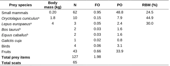
(32) In 65 culpeo fox scats, we found 14 different prey items including 12 mammals and 2 bird species. Small mammals, mainly rodent species, were the most frequently consumed prey item by this predator (FO = 0.95 and PO = 48.8) representing ¼ of the relative biomass intake (RBM = 24.5%). Rabbits were also frequently consumed by foxes (FO = 0.15, PO = 7.9), while hares were not as frequent (FO = 0.05, PO = 2.4%). Nevertheless, hares represented a considerable source of relative biomass (RBM = 30%). Fruits were found in a third of the feces analyzed (PO = 33.9). As the focus of this study was on predator-prey interactions, fruit presence was not considered for relative biomass analysis. Prey items considered as incidental or scavenging (i.e. livestock species and other carnivores), were not considered for this analysis. Nonetheless, they are all reported (Table 2).. Table 2. Prey composition of fox (L. culpaeus) in the study area, Machalí, central Chile, between 2012 and 2018. Results are reported as percentage of occurrence (PO), frequency of occurrence (FO), and relative biomass (RBM). Ungulates and carnivores were not included in relative biomass (RBM) calculation as they should be considered as incidental and or scavenging. Fruits were neither included as we focus on mammalian prey species interactions. Prey species Small mammals Oryctolagus. cuniculusa. Body mass (kg) 0.20. N. FO. PO. RBM (%). 62. 0.95. 48.8. 24.5. 1.8. 10. 0.15. 7.9. 44.9. 4. 30.0. 3. 0.05. 2.4. taurusb. 2. 0.03. 1.6. Equus caballusb. 2. 0.03. 1.6. Galictis cuja. 1. 0.02. 0.8. Birds. 4. 0.06. 3.1. Fruits. 43. 0.66. 33.9. Total prey items. 127. 1.98. Total scats a Introduced species. 65. Lepus Bos. b. europaeusa. Domestic species. 29.

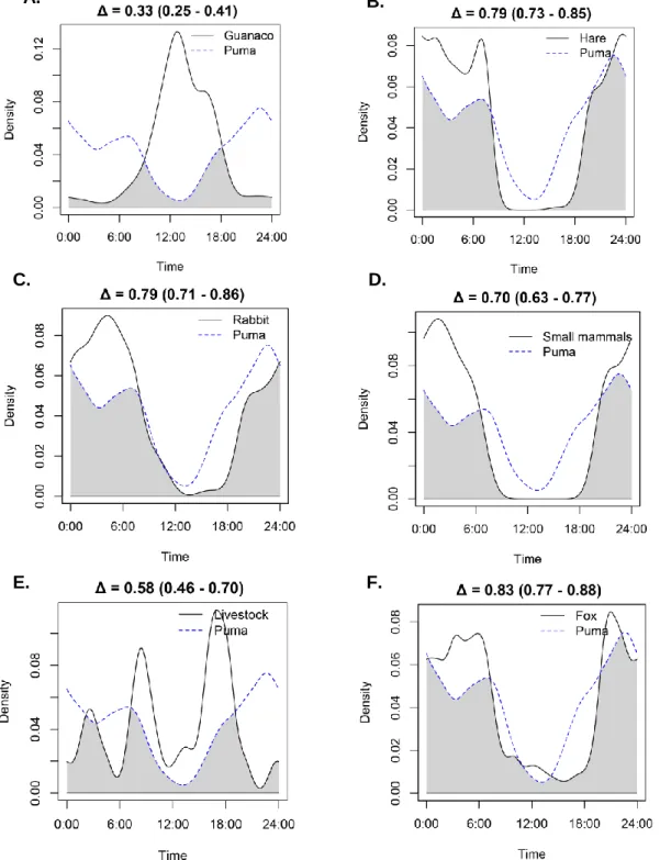
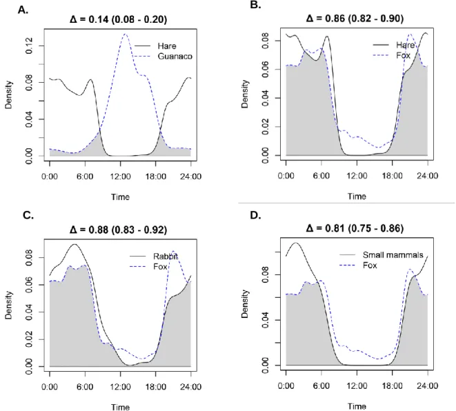
(33) Camera trap general results We obtained a total of 3,586 independent events (IE30’) from our focal species throughout autumn-winter seasons from 2013 to 2017. By year, we obtained 1,273 IE30’ in 2013, 1,690 IE30’ in 2015, and 543 IE30’ in 2017, with considerable sampling effort each sampling season (i.e. total camera nights per year on winter, 1,846, 4,956, and 2,536 respectively). The species with the largest amount of IE30’ was foxes (1,849), followed by hares (687), rabbits (329), small mammals (263), pumas (227), guanacos (170), and livestock (54). We also registered 7 IE30’ from pampas cat (Leopardus colocolo M.), and only 4 IE30’ from domestic dogs (Canis familiaris L.). Guanaco group size was observed to grow at the end of the season, often forming large groups up to 9 individuals (Appendix 2), with averages of 1.6 (March/April), 2.77 (April/May), 1.95 (May/June), 2.62 (June/July), and 3.2 (July/August) individuals per group observed in camera trap photographs. Daily activity pattern overlaps The higher activity pattern overlaps were found between fox and some of its potential preys, as rabbits (Δ = 0.88), followed by hares (Δ = 0.86), species that showed a predominantly nocturnal and crepuscular activity (Figure 4). Also, foxes showed a high activity pattern overlap with small mammals (Δ = 0.81). For the top predator in the study area, the puma, the highest activity pattern overlap was observed with fox (Δ = 0.83), followed by rabbits and hares (Δ = 0.79; Figure 3), small mammals (Δ = 0.70), livestock (Δ = 0.58), and guanaco (Δ = 0.33). This latter was the only one that showed a clearly diurnal activity pattern, having also a low activity pattern overlap with its main likely competitor, the hare (Δ = 0.14).. 30.

(34) A.. B.. C.. D.. E.. F.. Figure 3. Activity pattern overlaps between puma (P. concolor) and its preys: A. guanaco (L. guanicoe), B. hare (L. europaeus), C. rabbit (O. cuniculus), D. rodents, E. livestock and F. culpeo fox (L. culpaeus); in autumn-winter seasons in Río los Cipreses National Reserve, Central Chile, years 2013, 2015 and 2017. The y-axis shows kernel density estimation and x-axis shows time of day. Black line and dashed line represent species activity pattern being compared. Grey area represents activity overlap between both species being compared, and Δ corresponds to kernel index of overlap, showing 95% compatibility intervals inside parenthesis.. 31.

(35) A.. C.. B.. D.. Figure 4. Activity pattern overlaps between hares (L. europaeus) and guanacos (L. guanicoe) (A,) and between fox (L. culpaeus) and its preys: B. hare (L. europaeus), C. rabbit (O. cuniculus), and D. small mammals, in autumn-winter seasons in Río los Cipreses National Reserve, Central Chile, years 2013, 2015 and 2017. The y-axis shows kernel density estimation and x-axis shows time of day. Black line and dashed line represent species activity pattern being compared. Grey area represents activity overlap between both species being compared, and Δ corresponds to kernel index of overlap, showing 95% compatibility intervals inside parenthesis.. 32.

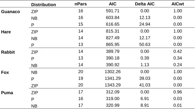
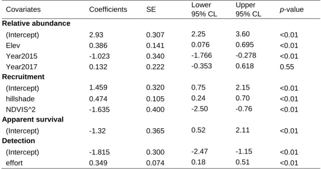
(36) Models results Guanaco After discarding models within <2 AIC units because of uninformative parameters included, only one model was considered competitive (Table 3). As expected from field observations, best model predictions showed guanacos to be mostly present in high altitudes (above 2000 m.a.s.l.) and likely outside the protected area in the first autumn month (Figure 7) and starting to progressively colonize the sites surveyed as the season entered winter months. This is reflected on a low initial abundance (λ = 0.023, SE = 0.07) and detection probability for each visit (p = 0.01, SE = 0.007) in the top model (Table 3). Detection probability increased by both, sampling effort (effort; ᵝ = 0.0492, SE = 0.010) and snow fall accumulation in each site (i.e. SNOWS; ᵝ = 1.456, SE = 0.0924; Figure 12), while recruitment probability increased only with higher hillshade values (ᵝ = 0.022, SE = 0.05). Each site included for guanaco analysis had, on average, a 44% probability to be colonized by the species (SE = 0.29), and approximately 74% probability to loss guanaco groups (SE = 0.19, Table 3), which reflect the intense movement of the species in the study site and period. Finally, the average snow accumulated for each site for the study period strongly increased guanaco abundance (SNOW; ᵝ = 6.08, SE = 3.01; Figure 14, Table 11). Hare Similar to guanacos, only one competitive model was selected (Table 3). Unlike guanacos, hares were regularly present in the study area, and most populated sites remained highly populated through the season (Figure 8), however, abundance progressively increase in those sites, as well as in neighbor sites. Moreover, initial abundance was the highest from all prey species (λ = 18.8, SE = 5.77), and its detection probability for each visit and site was not negligible (p = 0.14, SE = 0.036) (Table 3). Detection probability increased with number of camera nights per visit (effort; ᵝ = 0.349, SE = 0.074), whereas recruitment probability was higher on less shaded sites (hillshade; ᵝ = 0.474, SE = 0.105) and decreased with monthly changes in quadratic NDVI (NDVIS^2; ᵝ = -1.635, SE = 0.40) which descended as colder months approached. Furthermore, hare abundance increased on higher elevations (Elev; ᵝ = 0.386, SE = 0.141) and less hares where counted in year 2015 (ᵝ = -1.023, SE = 0.34, p-value < 0.01; Table 12, Figure 14), suggesting an abundance increase in recent years.. 33.

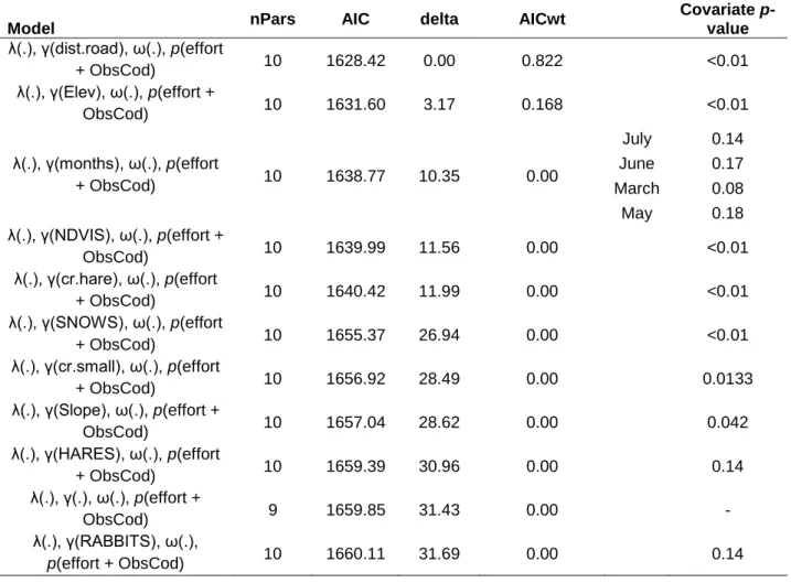
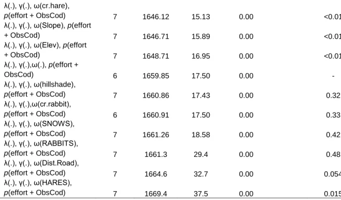
(37) Rabbit As well as for previous species, we selected only one competitive model for rabbit (Table 3). Rabbits relative abundance was lower than hares’ and restricted to few sites (Figure 9). This low movement between sites through months is reflected in the low colonization probability estimate in the best model fitted (γ = 0.005, SE = 0.008; Table 3). Detection probability was the highest among preys (p = 0.246, SE = 0.028), and it increased through the season within 10-day intervals (interval10; ᵝ = 0.50, SE = 0.115). As well as for guanaco and hare, recruitment was more likely in sites with higher hillshade values (ᵝ = 2.5, SE = 0.695). Sites with less slope hosted relatively more rabbits (Slope; ᵝ = -0.83, SE = 0.115; Table 13; Figure 14). Culpeo Fox Culpeo fox best model estimated relatively high abundance for the first month (March/April) in the area (λ = 13, SE = 2.27; Table 3). Furthermore, in average, fox abundance increased considerably throughout the season (γ = 3.46, SE = 0.47). This species was very conspicuous, showing high detection probability for each visit (p = 0.31, SE = 0.022). Detection was more likely with more sampling nights per visit (ᵝ = 0.571, SE = 0.094), and observers showed differences in their ability to detect this species (Table 14; Figure 15). Best model did not include any interaction of preys driving fox recruitment probability, as models fitted with abiotic covariates had more support in AIC analysis, nevertheless, hare capture rate (cr.hare) and small mammals capture rate (cr.small) covariates had very low pvalues in alternative models (Table 7). Higher slopes and longer distances to roads decreased culpeo fox’s recruitment probability (Slope; ᵝ = -0.465, SE = 0.143; Dist.Road; ᵝ = -0.465, SE = 0.143; Table 14). Hare abundance predictions for each month showed a positive interaction with fox apparent survival (ᵝ = 1.102, SE = 0.392), while sites at higher altitude where more unlikely to retain foxes (ᵝ = -2.547, SE = 1.051). Small mammal and hare capture rate also showed low p-values (and low AIC) in alternative single covariate models for fox apparent survival (Table 8). Abundance was better explained by biotic covariates, where sites predicted to hold higher rabbit abundance attracted more foxes (RABBITAB; ᵝ = 0.139, SE = 0.097), whereas Andean Steppe habitat hosted less foxes (ᵝ = -1.078, SE = 0.225; Figure 17). Despite it was not selected as abundance covariate in the best model, single-covariate model containing hare capture rate was highly ranked and had a low p-value (<0.01; Table 5).. 34.