Suggested method for heat transfer calculation during film condensation inside pipes with movable frontiers

Texto completo

(1)Mathematical Modelling of Engineering Problems Vol. 6, No. 3, September, 2019, pp. 449-454 Journal homepage: http://iieta.org/journals/mmep. Suggested Method for Heat Transfer Calculation During Film Condensation Inside Pipes with Movable Frontiers Yanán Camaraza-Medina1*, Yaniel García-Lovella1, Andres A. Sánchez-Escalona2, Elizaida Torres-Sarmiento3, Oscar M. Cruz-Fonticiella1, Osvaldo F. García-Morales4 1. Center of Energy Studies and Environmental Technology, Universidad Central “Marta Abreu” de Las Villas, 54440, Cuba Metallurgical Mining Higher Institute, Doctoral Research Program. 83330 Moa, Holguí n, Cuba 3 Department of Technical Assistence, School Buss Company, Segundo Frente, 93330, Santiago de Cuba, Cuba 4 Technical Sciences Faculty, Universidad de Matanzas, 44440, Cuba 2. Corresponding Author Email: [email protected] https://doi.org/10.18280/mmep.060317. ABSTRACT. Received: 20 June 2019 Accepted: 3 September 2019. This paper provides a second evaluation, with the intention of formulating an improved model that is capable of predicting the mean coefficients of heat transfer during condensation inside tubes with any orientation. This model has been developed through the application of transportable borders for the propagation of heat inside an elementary volume, up to the macro system considered. The theoretical model obtained leads to two basic dimensionless groups, which establish the study intervals that should be considered in the correlation of experimental quantities available, for the development of future experimental models.. Keywords: flow condensation, heat transfer coefficient, mathematical deduction, movable frontiers. 1. INTRODUCTION. correlation indexes obtained at present with the valid calculation procedures. This model has been obtained through the application of problems with mobile borders, for the propagation of heat in the confined space in the boundary layer inside the tubes, with any geometrical orientation.. Condensation is a mode of heat transfer involving saturated steam. Condensation occurs when the vapor finds a surface at a temperature below the saturation temperature, then when this event occurs; the agent undergoes a phase change, [1-5]. At present, several works are available, in which a detailed study of the correlation of several known models has been developed, as well as its index of uncertainty in the prediction of the average heat transfer coefficients. However, on the contrary, there are still divergences regarding the structure and way of grouping the variables, which should predict the condensation models, for this reason it is that about two dozen models are known, as well as the variables and asymmetrical groups that compose them [6-8]. Currently, Chato's expression is the one used to obtain the coefficient of heat transfer by condensation inside pipes. This method was developed for horizontal pipes, and in their correlation, several refrigerants and water were used. The Chato equation is valid for Reynolds numbers below 35000. Chato's model assumes that vapor has negligible velocity, so it does not provide heat to the stratified liquid at the bottom of the tube, and offers no resistance to it. The knowledge of this problem motivates the authors to develop an analysis methodology that considers the effect of steam drag and that also includes the effect of sub-cooling of the liquid, and that for others is as accurate as the methods currently used, [9- 12]. To solve this problem and its subsequent application to the condensation of vapors inside a tube with any geometric orientation, the authors combined the solution of the differential equation of temperature distribution with the differential relationship of the velocity profile. Based on the above, the authors define as the objective of this work to make a second attempt to present a model that allows improving the. 2. MATHEMATICAL CONSIDERATIONS 2.1 Eigenfunction expansions on boundary layer The elliptical operators are the elements that provide the closest natural analogy to the one-dimensional linear differential operators, which are shown in details in the works [2-4]. The operator 𝐿 = −∇2 is formally self-adjoint with respect to the inner product, then: ⟨𝜙, 𝜒⟩ = ∬ 𝜙 ∗ 𝜒𝑑𝑥𝑑𝑦. (1). This property given in Equation (1) follows from Green’s identity ∬Ω {𝜙 ∗ (−∇2 x) − (−∇2 ϕ)∗ 𝜒}𝑑𝑥𝑑𝑦 = ∫∂Ω{𝜙 ∗ (−∇x) − (−∇ϕ)∗ 𝜒}n𝑑𝑠 (2) In Equation (2) ∂Ω is the boundary of the region Ω and n is the outward normal on the boundary. By means of the method of separation of variables, it is possible to solve problems of eigenvalues, which include the operator of Laplace, for example, the problem of Dirichlet's eigenvalues requires that a group of eigenfunctions be determined and also that the operator's eigenvalues be defined. 𝐿 = −∇2 , D(L) = {𝜙 ∈ 𝐿2 [Ω]: 𝜙 = 0, on ∂Ω}. 449. (3).

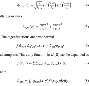
(2) Suppose Ω is the tube 0 ≤ 𝑙 ≤ 𝑙𝑥 , 0 ≤ 𝑟 ≤ 𝑟𝑥 . the normalized eigenfunctions are: 𝜙𝑛,𝑚 (𝑥) = √. 4 𝑙𝑥 𝑟𝑥. sin (. 𝑛𝜋𝑙 𝑙𝑥. ) sin (. 𝑚𝜋𝑟 𝑟𝑥. ). =. ∞. 1 2𝑛 𝜋 0.5𝑛. ∫ 𝑑𝑡 𝑡 0.5𝑛−2 𝑒 𝑡∙|𝑟−𝑟 0. (4). 1. 1. 𝑛−1. with eigenvalues 𝑛𝜋 2. 𝑚𝜋 2. 𝑙𝑥. 𝑟𝑥. 1−0.5𝑛. |𝑟 − 𝑟 ′ |2 1 𝑛 = 𝑛 0.5𝑛 Γ ( − 1) ( ) 2 𝜋 2 4 = (𝑛−2)𝑆. 𝜆𝑛,𝑚 (𝑥) = ( ) + (. ′ |2 ⁄4. (|𝑟−𝑟 ′ |). 𝑛−2. (12). In Eq. (12), the term Γ(x)is Euler’s gamma function:. ). (5) ∞. Γ(𝑥) = ∫0 𝑑𝑡 𝑡 𝑥−1 𝑒 𝑡. (13). The eigenfunctions are orthonormal And ∫ 𝜙𝑛,𝑚 𝜙𝑛′ ,𝑚′ 𝑑𝑥𝑑𝑦 = 𝛿𝑛𝑛′ 𝛿𝑚𝑚′ 2 [Ω]. and complete. Thus, any function in 𝐿. (6) Sn−1 =. can be expanded as. 𝑓(𝑥, 𝑦) = ∑∞ 𝑚,𝑛=1 𝐴𝑛𝑚 𝜙𝑛,𝑚 (𝑥, 𝑦). 𝑔(𝑟, 𝑟 ′ ) =. 𝑛=3. 1. Γ(𝑥) = Γ(𝑥 + 1) 𝑥. (15). (16). Together with 𝑎 𝑥 = 𝑒 𝑎 ln 𝑥 = 1 + 𝑎 ln 𝑥 + ⋯. (17). To examine the behavior of 𝑔(𝑟, 𝑟 ′ ) near 𝑛 = 2:. Once we known the eigenfunctions φn and eigenvales λn for −∇2 in a region Ω we can write down the Green function as =. ;. When studying the phenomena in two dimensions, it is noted that the Fourier integral turns out to be divergent for reduced values of thermal conductivity 𝑘. This divergence is possible to control if the dimensionless regularization techniques are applied. For this purpose, it is assumed that the number of samples n turns out to be a continuous variable, therefore it is possible to establish that:. 2.2 Applications of the Green functional. 𝑔(𝑟, 𝑟. 1 4𝜋|𝑟−𝑟 ′|. (8). As long as the Laplace operator can be isolated, it is possible to define a compact set in the form of a product of its own functions, given in the coordinate system 𝜉𝑖 such that theboundary becomes 𝜉𝑖 = 𝑐𝑜𝑛𝑠𝑡 . The compactness of the space in several dimensions is guaranteed by the integrity of the functions of each one-dimensional differential operator described by its own functions. Conversely, for other coordinates systems, the own functions when being separated are not functions of elementary character, reason why the Laplacian is composed then by a set of own functions of Dirichlet, which will be valid in any region of integration.. ′). (14). Eq. (14) is the surface area of the n-dimensional unit wall. For three dimensions, the equation (12) is transformed to:. (7). where 𝐴𝑛𝑚 = ∬ 𝜙𝑛,𝑚 (𝑥, 𝑦)𝑓 (𝑥, 𝑦)𝑑𝑥𝑑𝑦. 2πn⁄2 Γ(n⁄2). 1. ∑𝑛 𝜑𝑛 (𝑟)𝜑𝑛∗ (𝑟 ′ ) 𝜆𝑛. 𝑔(𝑟, 𝑟 ′ ) = 1 Γ(n⁄2) (1 − (n⁄2 − 1) ln(π|r − r ′ |2 ) + O[(n − 2)2 ]) 4𝜋 (n⁄2 − 1). = (9). 1. (. 1. 4𝜋 n⁄2−1. − 2 ln|r − r ′ | − ln π − γ + ⋯) (18). The Green function for the Laplacian in the entire ℝ𝑛 is givenby the sum over eigenfunctions ′ 𝑑 𝑛 𝑘 𝑒 𝑖𝑘∙(𝑟−𝑟 ). 𝑔(𝑟, 𝑟 ′ ) = ∫ (2𝜋)𝑛. 𝑘2. (10). Thus 𝑑𝑛 𝑘. ′. −∇2r 𝑔(𝑟, 𝑟 ′ ) = ∫ (2𝜋)𝑛 𝑒 𝑖𝑘∙(𝑟−𝑟 ) = 𝛿 𝑛 ∙ (𝑟 − 𝑟 ′ ). (11). Figure 1. Interior potential development of the Green functional. We can evaluate the integral given in Equation (11) or any 𝑛 by using Schwinger’s trick to turn the integrand into a Gaussian (see Figure 1): ∞. 𝑔(𝑟, 𝑟 ′ ) = ∫ 𝑑𝑠 ∫ 0 ∞. In Eq. (18) the term γ = −Γ ′ (1) = 0.5772 is the EulerMascheroni constant. The pole 1⁄(n⁄2 − 1) blast up at 𝑛 = 2, it is independent of position, however, this term can be incorporated and simplified, the − ln 𝜋 − 𝛾 into an undetermined additive constant. Then, the limit 𝑛 → 2 can be taken and we find:. 𝑑 𝑛 𝑘 𝑖𝑘∙(𝑟−𝑟 ′) −𝑠𝑘 2 𝑒 𝑒 (2𝜋)𝑛. 𝑛. 1 𝜋 1 ′ 2 = ∫ 𝑑𝑠 (√ ) 𝑒 −4𝑠𝑘∙|𝑟−𝑟 | 𝑛 𝑠 (2𝜋) 0. 450.

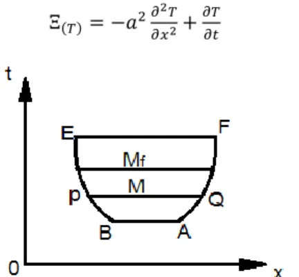
(3) 𝑔(𝑟, 𝑟 ′ ) =. 1 2𝜋. ln|r − r ′ | + const. ,. n=2. 𝜕𝜑 𝜕𝜓 − 𝜑 ) 𝑑𝑡] 𝜕𝑥 𝜕𝑥 𝜕𝜑 𝜕𝜓 − ∫𝐴𝑃 [𝜑𝜓𝑑𝑥 + 𝑎2 (𝜓 − 𝜑 ) 𝑑𝑡] = 0 𝜕𝑥 𝜕𝑥. (19). +𝑎2 (𝜓. The inclusion of a constant value in Eq. (19) does not influence on the Green- function property, so we can choose any convenient value for it. Although this procedure allows to reduce the uncertainty index of the coefficient of thermal conductivity, press in the Fourier integral, in the measure that the value of the thermal conductivity is increased, a problem of convergence of the function is generated, however, the Green function in ℝ3 allows us to solve for 𝜙(𝑟) in the equation −∇2 𝜑 = 𝑞(𝑟). In Eq. (23), the term the problem.. When the Green´s Equation is equal to zero, then the source function 𝜓 = 𝐺0 (𝑥, 𝑡, 𝜉, 𝜏) is obtained. This equation in the infinite line is:. when 𝑛 = 1 the problem is reduced to the study of a volume of elementary control of a section of the tube. Any section is taken along the tube, to establish the control volume, (see Figure 1), considering in a first approximation attempt that the flow has one-dimensional sharing, which simplifies the study, since then the axial components they are a priority, while the radial elements pass to a secondary role, so they can be neglected. In the elementary section considered for the study (see Figure 2), the process is assumed in steady state, then, the input is then defined by the PB segment, while the AQ segment becomes the output zone of the heat flow. For this reason, the heat flux, its trajectory is known, but the arbitrary function that is capable of describing it is unknown, but it can be described in an approximate way, which can be expressed as:. 𝜓 = 𝐺0 (𝑥, 𝑡, 𝜉, 𝑡) =. 𝜕2 𝑇 𝜕𝑥 2. +. 𝜕𝑇 𝜕𝑡. 1 2√𝜋𝑎2 (𝑡−𝜏). 𝑒 2. −. (𝑥−𝜉)2 4𝑎2 (𝑡−𝜏). (24). Assuming that the solution to the heat transfer problem inside the selected elementary volume is described by 𝜑(𝑥, 𝑡 + ℎ), where ℎ > 0, then it is possible to formulate the solution of the heat transfer problem 𝜑(𝑥, 𝑡) Substituting 𝑥 − ℎ = 𝜉 and 𝑡 = 𝜏 + ℎ, the Tijonov’s infinite line (Equation (24)) is transformed to: 𝜓 = 𝐺0 (𝑥, 𝑡) =. 1 2√𝑥𝑎2 ℎ2. 𝑒. −. (2𝑥−ℎ) 4𝑎2 ℎ. (25). The solution of the desired problem can be generated from the simplification given previously for the elementary section PABQ, applying for that purpose the criterion of the minimum energy principle, finding for each integral section its corresponding minimum, which is possible when applying the following substitutions:. (21). By applying the principle of maximum value, it is possible to establish that in the problem studied there is one and only one solution, which turns out to be continuous and maximum, then the Green’s functional differential can write as: Ξ(𝑇) = −𝑎2.  (x, t ) is the heat transfer solution for. 2.3 Applications of the finite element procedures to the problems solution. (20). 𝑥 = 𝑋1 (𝑡) for 𝑃𝐵 𝑥 = 𝑋2 (𝑡) for 𝐴𝑄. (23). 1. 𝜑(𝑥, 𝑡). 2√𝜋𝑎 2 ℎ2. 𝑒. (2𝑥−ℎ)2 4𝑎2 ℎ. −. =𝜔 ̅. (26). or: (22) 1 2√𝜋𝑎2 ℎ. 𝑒 2. (2𝑥−ℎ)2 𝜕𝜑(𝑥,𝑡) 4𝑎2 ℎ. −. 𝜕𝑥. 𝜕(. − 𝜑(𝑥, 𝑡). 1 2√𝜋𝑎2 ℎ2. 𝑒. (2𝑥−ℎ)2 − 4𝑎2 ℎ ). 𝜕𝑥. 𝜔. = (27). that proves to be equivalent: 𝜔 ̅. 𝜕𝜑 𝜕𝑥. − 𝜑(𝑥, 𝑡). ̅ 𝜕𝜔 𝜕𝑥. =𝜔. (28). Substituting Eq. (27) and Eq. (28), in Eq. (23): Figure 2. Model problem and elementary volumes employed. ̅𝑑𝑥 − ∫𝐴𝑄 𝜔 ̅𝑑𝑥 + ∫𝑃𝐵 𝜔. The selected elementary section PAQB can be divided into four linear sections, called PB, AQ, BQ and AP. For any of these linear sections, the solution of the differential equation (12) and its combination with the integral criterion of Green, allows obtaining an integral complex, which allows solving the problem on the studied boundary at any point inside and outside the volume of control, [10-11]:. ∫𝐵𝑄 [. 𝑎2 (𝜔. 𝐴𝑄. 𝜕𝑥 𝜕𝜑(𝑥,𝑡) 𝜕𝑥. −𝜑(𝑥, 𝑡). 𝜕𝜔 𝜕𝑥. ) 𝑑𝑡] = 0. (29). By using finite element techniques, it is possible to reduce equation (30) to a control volume composed of linear finite elements. A triangular finite element composed of three nodes is selected (one-dimensional triangular element). The onedimensional triangular element has a node at the center and the. ∫ 𝜑𝜓𝑑𝑥 − ∫ 𝜑𝜓𝑑𝑥 + ∫ [𝜑𝜓𝑑𝑥 𝑃𝐵. 𝜔𝑑𝑥 𝜕𝜔 𝜕𝜑(𝑥,𝑡) − 𝜑(𝑥, 𝑡) ) 𝑑𝑡] − ∫𝐴𝑃 [𝜔𝑑𝑥 + 𝜕𝑥 +𝑎2 (𝜔. 𝐵𝑄. 451.

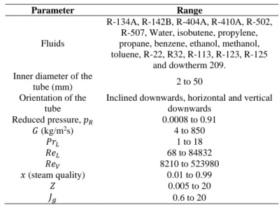
(4) two remaining nodes are located at both ends of the finite element [3], see Figure 3.. 3. EXPERIMENTAL VALIDATION 3.1 Experimental validation of the new model The dimensionless Shah parameter is defined by Equation (53) [17]: 𝑍=(. 1−𝑥 0.8 𝑥. ). 𝑃𝑟𝐿0.4. (38). The combination of the Equations (37) and (38) provide the applicability range for vertical, inclined and horizontal tube. Figure 3. Representation of a quadratic one-dimensional element. For vertical and inclined tubes Zone 1 𝐽𝑔 ≥. The form functions for this type of elements are: 1 𝑁1 = − 𝜉(1 − 𝜉); 𝑁2 = (1 + 𝜉)(1 + 𝜉); 2 1 𝑁3 = 𝜉(1 + 𝜉). Zone 2 0.927𝑒 (−0.0868𝑍 (30). 2. 1. 1. 2. 2. 𝜕𝑉𝑋 𝜕𝑥. ). (1 − 2𝑥 +. = 𝑎(1 − 2𝑥 + 𝑥. 2 )2. + 3𝜇 (. 𝜕𝑥. (31). ). 1. 1. 2. 2. 2. 𝜕𝑉𝑋 2 𝜕𝑥. ). (32). 1. 1. 2. 2. 2. (33). 𝜕𝑉𝑋 2 𝜕𝑥. (42) (43). In investigations carried out, the authors [15] show that Eqns. (39) to (43) can be used in the determination of a model for the calculation of the average coefficient of heat transfer by condensation, valid for any spatial configuration of the tube. This procedure allowing also reducing the uncertainty index up to 13 % for vertical and inclined tubes, while for horizontal tubes the average error is reduced up to 11.8 %.. Segment AQ Entry − (− 𝑥 + 𝑥 2 ) 𝑉𝑋 = −𝑎 (− 𝑥 + 𝑥 2 ) + −3𝜇 (. (41). 3.2 Elements to consider for the application of the developed model. Exit ( 𝑥 + 𝑥 2 ) 𝑉𝑋 = 𝑎 ( 𝑥 + 𝑥 2 ) + 3𝜇 (. −1.165 ). (40). An extended summary of the validity range in which the developed model provides an adequate fit is given in Table 1, [15].. 2. 𝜕𝑉𝑋 2. 1 2.37𝑍+0.728. Zone 2 𝐽𝑔 > 0.979(𝑍 + 0.262)−0.618. Intermediate 𝑥 2 )𝑉𝑥. (39). For horizontal pipes Zone 1 𝐽𝑔 ≤ 0.979(𝑍 + 0.262)−0.618. Segment PB Entry (− 𝑥 + 𝑥 2 ) 𝑉𝑋 = 𝑎 (− 𝑥 + 𝑥 2 ) + 3𝜇 (. < 𝐽𝑔 <. Zone 3 𝐽𝑔 ≤ 0.927𝑒 (−0.0868𝑍. The approximate procedures for the solutions of the problems is obtained between the analysis of each individual segment in the given control volume (see figure 2), combining the Equations (30) and (29).. 2. −1.165 ). 1 2.37𝑍+0.728. ) (34). Table 1. Validity range for the proposal model. Intermediate −(1 + 2𝑥 + 𝑥 2 )𝑉𝑥 = −𝑎(1 + 2𝑥 + 𝑥 2 )2 − 3𝜇 (. 𝜕𝑉𝑋 2 𝜕𝑥. ). Parameter. (35). Exit. Fluids 1. 1. 2. 2. 2. − ( 𝑥 + 𝑥 ) 𝑉𝑋 = −𝑎 ( 𝑥 + 𝑥 ) − 3𝜇 ( 2. 2. 𝜕𝑉𝑋 2 𝜕𝑥. ). (36) Inner diameter of the tube (mm) Orientation of the tube Reduced pressure, 𝑝𝑅 𝐺 (kg/m2s) 𝑃𝑟𝐿 𝑅𝑒𝐿 𝑅𝑒𝑉 𝑥 (steam quality) 𝑍 𝐽𝑔. The simultaneous solution of the Equation (31) to (36) allows obtaining than the final solution is dependent of one dimensionless group, known as dimensional velocity (1/𝐽𝑔 ) [13] 𝐽𝑔 =. 𝑥𝐺 √𝑔𝑑𝜌𝑉 (𝜌𝐿 −𝜌𝑉 ). (37). For inclined and vertical tubes, the use of the criterion of weak solutions allows to obtain equality of results with respect to that obtained in Eq. (37), [14-16].. Range R-134A, R-142B, R-404A, R-410A, R-502, R-507, Water, isobutene, propylene, propane, benzene, ethanol, methanol, toluene, R-22, R32, R-113, R-123, R-125 and dowtherm 209. 2 to 50 Inclined downwards, horizontal and vertical downwards 0.0008 to 0.91 4 to 850 1 to 18 68 to 84832 8210 to 523980 0.01 to 0.99 0.005 to 20 0.6 to 20. Table 2 offers a comparison of the index of correlation obtained when compare the experimental available data with. 452.

(5) the obtained results by means of the uses of a group of existing models in literature [15, 21]. When verifying the given results, it could be verified that the proposed model evidences better values of adjustment, with an average error of the 15 %.. [2]. Table 2. Comparison of the some models with experimental values % average deviation in vertical and inclined tubes – – – – 15.7 – – 13.0. [3]. For vertical tubes, in the dispensable literature, only have a suitable model to predict the heat transfer coefficients, the Shah's equation, for this reason, in this paper, only are executed comparisons with this model. finding a deviation of 15.7 %, which is coincident with the 15.8 % showed in the original publication of the method [19-23].. [5]. Model Bohdal [11] Dobson-Chato [9] Akers et al. [17] Carpenter-Colburn [9] Shah [7] Tandon [12] Cavallini [10] Camaraza et al. [21]. % average deviation in horizontal tubes 14.9 14.3 18.6 19.9 13.9 21.2 14.6 11.8. [4]. [6]. 4. CONCLUSIONS The methods required for the mathematical deduction of a new model were developed, applying for this purpose the criterion of mobile boundaries of Green. The construction of the mathematical model was obtained with a process based on finite element techniques, determining for this purpose two dimensionless groups, obtaining from these a new model that allows reducing the uncertainty in the calculation of the average transfer coefficient of heat by condensation inside pipes. The adequacy of the differential criterion of the profile of velocities in the interior of tubes and their subsequent combination with the differential equation of the temperature profile, it is possible to execute it by means of the use of the mathematical technologies propitiated by the method of mobile borders. This procedure allows including the effect of the propagation of heat in a two-dimensional confined space, with any spatial orientation. The developed model is valid for horizontal, vertical and inclined tubes. The developed model was tested with similar solutions provided by other authors, and a better correlation index was found, with an average error of 11.8 % for horizontal tubes and 13 % for inclined and vertical tubes.. [7]. [8]. [9] [10]. [11]. [12] ACKNOWLEDGMENT [13] The authors give special thanks to Dr. Angel M. Rubio Gonzales, for the assistant in this paper. REFERENCES. [14]. [1] Will, J.B., Kruyt, N.P., Venner, C.H. (2017). An experimental study of forced convective heat transfer.. 453. International Journal of Heat and Mass Transfer, 109: 1059-1067. http://doi.org/10.1016/j.ijheatmasstransfer.2017.02.028. Liu, D., Zheng, Y., Moore, A., Ferdows, M. (2017). Spectral element simulations of three dimensional convective heat transfer. International Journal of Heat and Mass Transfer, 111: 1023-1038. http://doi.org/10.1016/j.ijheatmasstransfer.2017.04.066 Camaraza-Medina, Y., Rubio-Gonzales, A.M., CruzFonticiella, O.M., Garcia-Morales, O.F. (2017). Analysis of pressure influence over heat transfer coefficient on air cooled condenser. Journal Européen des Systems Automatisés, 50(3): 213-226. http://dx.doi.org/10.3166/jesa.50.213-226 Camaraza-Medina, Y., Rubio-Gonzales, A.M., CruzFonticiella, O.M., García-Morales, O.F. (2018). Simplified analysis of heat transfer through a finned tube bundle in air cooled condenser. Mathematical Modelling of Engineering Problems, 5(3): 237-242. https://doi.org/10.18280/mmep.050316 Medina, Y.C., Fonticiella, O.M.C., Morales, O.F.G. (2017). Design and modelation of piping systems by means of use friction factor in the transition turbulent zone. Mathematical Modelling of Engineering Problems, 4(4): 162-167. https://doi.org/10.18280/mmep.040404 Rabiee, R., Désilets, M., Proulx, P., Ariana, M., Julien, M. (2018). Determination of condensation heat transfer inside a horizontal smooth tube. International Journal of Heat and Mass Transfer, (124): 816-828. https://doi.org/10.1016/j.ijheatmasstransfer.2018.04.012 Shah, M.M. (1979). A general correlation for heat transfer during film condensation inside pipes. International Journal of Heat and Mass Transfer, 22(4): 547-556. https://doi.org/10.1016/0017-9310(79)90058-9 Lee, Y.G., Jang, Y.J., Choi, D.J. (2017). An experimental study of air–steam condensation on the exterior surface of a vertical tube under natural convection conditions. International Journal of Heat and Mass Transfer, (104): 1034-1047. http://dx.doi.org/10.1016/j.ijheatmasstransfer.2016.09.0 16 Dobson, M.K., Chato, J.C. (1998). Condensation in smooth horizontal tubes. Journal Heat Transfer, 120(1): 193-213. http://dx.doi.org/10.1115/1.2830043 Cavallini, A., Col, D.D., Doretti, L., Matkovic, M., Rossetto, L., Zilio, C., Censi, G. (2006). Condensation in horizontal smooth tubes: A new heat transfer model for heat exchanger design. Heat Transfer Engineering, 27(8): 31-38. https://doi.org/10.1080/01457630600793970 Bohdal, T., Charun, H., Sikora, M. (2012). Heat transfer during condensation of refrigerants in tubular minichannels. Archives of Thermodynamics, 33(2): 3-22. http://dx.doi.org/10.2478/v10173-012-0008-x Camaraza, Y. (2017). Introducción a la termo transferencia. Editorial Universitaria, La Habana. Medina, Y.C, Khandy, N.H., Fonticiella, O.M.C., Morales, O.F.G. (2017). Abstract of heat transfer coefficient modelation in single-phase systems inside pipes. Mathematical Modelling of Engineering Problems, 4(3): 126-131. https://doi.org/10.18280/mmep.040303 Medina, Y.C., Khandy, N.H., Carlson, K.M., Fonticiella, O.M.C., Morales, O.F.G. (2018). Mathematical modeling of two-phase media heat transfer coefficient in air-cooled condenser systems. International Journal of.

(6) [15]. [16]. [17]. [18]. [19]. [20]. [21]. [22]. [23]. Heat and Technology, 36(1): 319-324. https://doi.org/10.18280/ijht.360142 Camaraza-Medina, Y., Hernandez-Guerrero, A., Luviano-Ortiz, J.L., Mortensen-Carlson, K., CruzFonticiella, O.M., García-Morales, O.F. (2019). New model for heat transfer calculation during film condensation inside pipes. International Journal of Heat Mass Transfer, 128: 344-353. https://doi.org/10.1016/j.ijheatmasstransfer.2018.09.012 Ali, H.M., Qasim, M.Z., Ali, M. (2016), Free convection condensation heat transfer of steam on horizontal square wire wrapped tube. International Journal of Heat and Mass Transfer, 98: 350-358. https://doi.org/10.1016/j.ijheatmasstransfer.2016.03.053 Akers, W.W., Deans, H.A., Crosser, O.K. (1959). Condensing heat transfer within horizontal tubes. Chemical Engineering Progress Symposium Series, 55(29): 171-176. O’Neill, L., Balasubramaniam, R., Nahra, H.K., Hasan, M.M., Mudawar, I. (2019). Flow condensation heat transfer in a smooth tube at different orientations: Experimental results and predictive models. International Journal of Heat and Mass Transfer, 140: 533-563. https://doi.org/10.1016/j.ijheatmasstransfer.2019.05.103 Camaraza-Medina, Y., Cruz-Fonticiella, O.M., GarcíaMorales, O.F. (2019). New model for heat transfer calculation during fluid flow in single phase inside pipes. Thermal Science and Engineering Progress, 11: 162-166. https://doi.org/10.1016/j.tsep.2019.03.014 Camaraza-Medina, Y., Khandy, N.H., Carlson, K.M., Cruz-Fonticiella, O.M., Garcí a-Morales, O.F., ReyesCabrera, D. (2018). Evaluation of condensation heat transfer in air-cooled condenser by dominant flow criteria. Mathematical Modelling of Engineering Problems, 5(2): 76-82. https://doi.org/10.18280/mmep.050204 Camaraza-Medina, Y., Hernandez-Guerrero, A., Luviano-Ortiz, J.L., Cruz-Fonticiella, O.M., GarcíaMorales, O.F. (2019). Mathematical deduction of a new model for calculation of heat transfer by condensation inside pipes. International Journal of Heat Mass Transfer, 141: 180-190. https://doi.org/10.1016/j.ijheatmasstransfer.2019.06.076 Camaraza-Medina, Y., Mortensen-Carlson, K., Guha, P., Rubio-Gonzales, A.M., Cruz-Fonticiella, O.M., GarcíaMorales, O.F. (2019). Suggested model for heat transfer calculation during fluid flow in single phase inside pipes (II). International Journal of Heat and Technology, 37: 257-266. https://doi.org/10.18280/ijht.370131 Camaraza-Medina, Y., Cruz Fonticiella, O.M., GarcíaMorales, O.F. (2018). Predicción de la presión de salida de una turbina acoplada a un condensador de vapor refrigerado por aire. Centro Azúcar, 45(1): 50-61.. NOMENCLATURE 𝑎 𝐶𝑝 𝑑 𝐺 𝑔 ℎ𝑓𝑔 ℎ ℎ𝑇 ℎ𝐶 ℎ𝑚𝑒𝑑 𝐽𝑔 𝑘 𝑘𝐿 𝑃𝑟𝐿 𝑝𝑅 𝑅𝑒𝐿 𝑅𝑒𝑉 𝑇 ∆𝑇 𝑇𝑠𝑎𝑡 TP 𝑉 𝑉𝑀𝑎𝑥 𝑉𝑥 𝑉𝑦 𝑉𝑧 𝑥 𝑍. Thermal diffusivity, m2∙s-1 Specific heat, J∙kg-1∙K-1 Equivalent inner tube diameter, m Mass flux, kg∙m-2∙s-1 Gravitational acceleration, m∙s-2 Latent heat of vaporization, J∙kg-1. K-1 Single-phase heat transfer coefficient, kg∙m-1∙K-1∙s-1 Two-phase heat transfer coefficient, kg∙m-2∙s-3∙K-1 Single-phase heat transfer coefficient, kg∙m-2∙s-3∙K-1 Experimental measured value, kg∙m-2∙s-3∙K-1 Dimensionless velocity Fluid thermal conductivity, W∙m-1∙K-1 Fluid thermal conductivity for single-phase, W∙m-1∙K-1 Prandtl number for single-phase Reduced pressure Liquid Reynolds number Vapor Reynolds number Mean fluid temperature, °C Temperature difference across the condensate film Saturation temperature, °C Wall temperature, °C Velocity profile, m∙s-1 Maximum velocity, m∙s-1 Velocity component in x axis, m∙s-1 Velocity component in y axis, m∙s-1 Velocity component in z axis, m∙s-1 Thermodynamic vapor quality Dimensionless Shah parameter. Greek symbols.  µ 𝜃 𝜌 𝜉 𝑣 𝛿 φ 𝜓 𝜏 𝜔. Thermal expansion coefficient, K-1 Dynamic viscosity, kg∙m-1∙s-1 Tubes inclination respect to horizontal line Density, kg∙m-3 Number of intervals in function form, Equation (30) Liquid kinematic viscosity, m2∙s-1 Film thickness of boundary layer, m Solution of the heat transfer problem, (Equation (26)) Source function, (Equation (24)) Temperature in Green’s functional, (Equation (22)) Substituting term employed in Equation (28). Subscripts 𝐿 V. 454. Liquid Vapor.

(7)