Computational properties of delay coupled systems

Texto completo

(1)DOCTORAL THESIS 2015. COMPUTATIONAL PROPERTIES OF DELAY-COUPLED SYSTEMS. Miguel Angel Escalona Morán.

(2) DOCTORAL THESIS 2015 Doctoral Program of Physics. COMPUTATIONAL PROPERTIES OF DELAY-COUPLED SYSTEMS. Miguel Angel Escalona Morán Thesis Supervisor: Claudio R. Mirasso Santos Thesis Co-Supervisor: Miguel Cornelles Soriano. Doctor by the Universitat de les Illes Balears.

(3) COMPUTATIONAL PROPERTIES OF DELAY-COUPLED SYSTEMS Miguel Angel Escalona Morán Tesis realizada en el Instituto de Física Interdisciplinar y Sistemas Complejos (IFISC) y presentada en el Departamento de Física de la Universitat de les Illes Balears.. Supervisor: Prof. Claudio R. Mirasso Santos Co-Supervisor: Dr. Miguel Cornelles Soriano. iii.

(4)

(5) Tesis Doctoral presentada por Miguel Angel Escalona Morán para optar al título de Doctor, en el Programa de Física del Departamento de Física de la Universitat de les Illes Balears, realizada en el IFISC bajo la dirección de Claudio Mirasso, catedrático de universidad y Miguel Cornelles Soriano, contratado postdoctoral CAIB. Visto bueno Director de la tesis. Prof. Claudio Mirasso Co-Director de la tesis. Dr. Miguel Cornelles Soriano Doctorando. Miguel Angel Escalona Morán Palma, Junio de 2015. v.

(6) vi.

(7) Summary of the research work In this research work we study the computational properties of delay-coupled systems. In particular, we use a machine learning technique known as reservoir computing. In machine learning, a computer learns to solve di↵erent tasks using examples and without knowing explicitly their solution. For the study of the computational properties, a numerical toolbox, written in Python, was developed. This toolbox allows a fast implementation of the di↵erent scenarios described in this thesis. Using a reservoir computer, we studied several computational properties, focusing on its kernel quality, its ability to separate di↵erent input samples and the intrinsic memory capacity. This intrinsic memory is related to the delayedfeedback of the reservoir. We used a delay-coupled system as reservoir to study its computational ability in three di↵erent kinds of tasks: system’s modeling, time-series prediction and classification tasks. The system’s modeling task was performed using the Nonlinear Autoregressive Moving Average (of ten steps), NARMA10. The NARMA10 model creates autoregressive time series from a set of normally distributed random sequences. The reservoir computer learns how to emulate the system using only the sequence of random numbers and the autoregressive time series, but without knowing the equations of the NARMA10. The results of our approach are equivalent to those published by other authors and show the computational power of our method. For the time-series prediction tasks, we used three kinds of time series: a model that gives the variations in temperature of the sea surface that provoke El Niño phenomenon, the Lorenz system and the dynamics of a chaotic laser. Di↵erent scenarios were explored depending on the nature of the time series. For the prediction of the variation in temperature of the sea surface, we perform estimations of one, three and six months in advance. The error was measured as. vii.

(8) the Normalized Root Mean Square Error (NRMSE). For the di↵erent prediction horizons, we obtained errors of 2%, 8% and 24%, respectively. The classification tasks were carried out for a Spoken Digit Recognition (SDR) task and a real-world biomedical task. The SDR was used to illustrate different scenarios of a machine learning problem. The biomedical task consists on the automatic classification of heartbeats with cardiac arrhythmias. We use the MIT-BIH Arrhythmia database, a widely used database in cardiology. For comparison purposes, we followed the guidelines of the Association for the Advancement of Medical Instrumentation for the evaluation of arrhythmia-detector algorithms. We used a biostatistical learning process named logistic regression that allowed to compute the probability that a heartbeat belongs to a particular class. This is in contrast to the commonly used linear regression. The results obtained in this work show the versatility and efficiency of our implemented reservoir computer. Our results are equivalent and show improvement over other reported results on this problem under similar conditions and using the same database. To enhance the computational ability of our delay-coupled system, we included a multivariate scheme that allows the consideration of di↵erent variables of a system. We evaluated the influence of this multivariate scenario using a timeseries prediction and the classification of heartbeat tasks. The results show improvement in the performance of the reservoir computer in comparison with the same tasks in the univariate case.. viii.

(9) Resumen del trabajo de investigación En esta tesis se estudian las propiedades computacionales de sistemas acoplados con retraso. En particular la técnica de machine learning, conocida como reservoir computing, es utilizada. En esta técnica el ordenador aprende a resolver tareas a partir de ejemplos que se han dado previamente pero sin indicarle de forma explícita la forma de resolver estos problemas. El desarrollo de este trabajo incluye la creación de una herramienta computacional, escrita en lenguaje Python para la ejecución de los diferentes escenarios presentados en este trabajo. Con la implementación de un sistema acoplado con retraso, hemos estudiado las propiedades de cómputo de este tipo de sistemas, interesándonos principalmente en la calidad del sistema acoplado, su habilidad de separación de elementos distintos y su capacidad intrínseca de memoria, la cual está asociada a la presencia de una retroalimentación retrasada. El sistema se ha usado para demostrar el poder de cálculo que ofrecen los sistemas acoplados con retraso. Se utilizaron tres tipos de tareas: modelado, predicción de series de tiempo y clasificación. El modelado se realizó utilizando el sistema Nonlinear Autoregressive Moving Average de 10 pasos (NARMA10). Este sistema, construye series temporales autoregresivas a partir de series de números aleatorios. El ordenador basado en reservoir aprende a emular este sistema (sin conocer de forma explícita las ecuaciones del mismo) a partir de las secuencias de números aleatorios y las series temporales autoregresivas. Los resultados obtenidos son equivalentes a los publicados por otros autores, demostrando el poder computacional de este método. Para la predicción de series temporales se usaron modelos de variación de temperatura que provocan la aparición del fenómeno de El Niño, el sistema de Lorenz en régimen caótico y la dinámica de un laser caótico. Las estimaciones de series temporales se realizaron bajo diversas circunstancias dependiendo de la naturaleza de las series. Para el caso de El Niño, se realizaron predicciones a uno, ix.

(10) tres y seis meses con errores de estimación, determinados por el Normalized Root Mean Square Error (NRMSE) de 2%, 8% y 24%, respectivamente. Como primera tarea de clasificación, se utilizó la tarea de Spoken Digit Recognition y se utilizó para ilustrar diferentes escenarios posibles de un sistema acoplado con retraso. La segunda tarea de clasificación y la mas exhaustiva, se realizó en un problema real de origen biomédico: la clasificación de latidos cardiacos para el caso de arritmias. Se utilizo la base de datos MIT-BIH Arrhythmia la cual ha sido ampliamente usada en cardiología. Por motivos de comparación de resultados, se siguieron las recomendaciones dadas por la Association for the Advancement of Medical Instrumentation para la evaluación de algoritmos detectores de arritmias. Se utilizo un método de entrenamiento del reservoir computer llamado regresión logística en lugar del comúnmente usado: la regresión lineal. La regresión logística nos permite obtener como resultado la probabilidad de que un latido cardiaco pertenezca a una clase u a otra. Los resultados obtenidos demuestran la versatilidad y eficacia de nuestro método de calculo, ya que son equivalentes e incluso mejores a los resultados publicados por otros trabajos bajo circunstancias similares de evaluación y utilizando la misma base de datos. Para mejorar la capacidad de computación del sistema con retraso, se incluyeron variables dinámicas adicionales en nuestro sistema para evaluar el efecto en la predicción de series de tiempo y la clasificación de latidos cardíacos. Los resultados mostraron una mejora sustancial en comparación con el caso en que sólo una variable o canal del electrocardiograma fue usado para realizar la tarea dada.. x.

(11) Resum del treball de recerca En aquesta tesi s’estudien les propietats computacionals de sistemes acoblats amb retard. En particular, hem utilitzat la tècnica de "machine learning" coneguda com reservoir computing. En aquesta tècnica, l’ordinador aprèn a resoldre tasques a partir d’exemples que s’han donat prèviament però sense indicar-li de forma explícita la forma de resoldre aquests problemes. El desenvolupament d’aquest treball inclou la creació d’una eina computacional, escrita en llenguatge Python per a l’execució dels diferents escenaris presentats en aquest treball. Amb la implementació d’un sistema acoblat amb retard, hem estudiat les propietats de còmput d’aquest tipus de sistemes, interessant-nos principalment en la qualitat del sistema acoblat, la seva habilitat de separació d’elements diferents i la seva capacitat intrínseca de memòria, la qual està associada a la presència d’una retroalimentació retardada. El sistema s’ha fet servir per demostrar el poder de càlcul que ofereixen els sistemes acoblats amb retard. Es van utilitzar tres tipus de tasques: modelatge, predicció de sèries de temps i classificació. El modelatge es va realitzar utilitzant el model "Nonlinear Autoregressive Moving Average" de 10 passos (NARMA10). Aquest model, construeix sèries temporals autoregresivas a partir de sèries de nombres aleatoris. L’ordinador basat en "reservoir computing" aprèn a emular aquest model (sense conèixer de forma explícita les equacions del mateix) a partir de les seqüències de nombres aleatoris i les sèries temporals autoregresivas. Els resultats obtinguts són equivalents als publicats per altres autors, demostrant el poder computacional d’aquest mètode. Per a la predicció de sèries temporals es van usar models de variació de temperatura que provoquen l’aparició del fenomen de El Niño, el sistema de Lorenz en règim caòtic i la dinàmica d’un làser caòtic. Les estimacions de sèries temporals es van realitzar sota diverses circumstàncies depenent de la naturalesa de les sèries. Per al cas d’El Niño, es van realitzar prediccions a un, tres i sis mesos. xi.

(12) amb errors d’estimació, determinats pel "Normalized Root Mean Square Error" (NRMSE) de 2%, 8% i 24%, respectivament. Com a primera tasca de classificació, es va utilitzar la tasca de "Spoken Digit Recognition" i s’han il·lustrat diferents configuracions possibles d’un sistema acoblat amb retard. La segona tasca de classificació i la més exhaustiva, es va realitzar en un problema real d’origen biomèdic: la classificació de batecs cardíacs per al cas d’arítmies. Es va utilitzar la base de dades "MIT-BIH Arrhythmia", la qual ha estat àmpliament usada en cardiologia. Per motius de comparació de resultats, es van seguir les recomanacions donades per la "Association for the Advancement of Medical Instrumentation" per a l’avaluació d’algoritmes detectors d’arítmies. Es va utilitzar un mètode d’entrenament del reservoir computer anomenat regressió logística en lloc del comunament usat: la regressió lineal. La regressió logística ens permet obtenir com a resultat la probabilitat que un batec cardíac pertanyi a una classe o a una altra. Els resultats obtinguts demostren la versatilitat i eficàcia del nostre mètode de càlcul, ja que són equivalents i fins i tot millors als resultats publicats per altres treballs sota circumstàncies similars d’avaluació i fent servir la mateixa base de dades. Per millorar la capacitat de computació del sistema amb retard, es van incloure variables dinàmiques addicionals en el nostre sistema per avaluar l’efecte en la predicció de sèries de temps i la classificació de batecs cardíacs. Els resultats van mostrar una millora substancial en comparació amb el cas en que només una variable o canal de l’electrocardiograma va ser usat per realitzar la tasca donada.. xii.

(13) List of Publications Published 1. M.C. Soriano, D. Brunner, M. Escalona-Morán, C. R. Mirasso and I. Fischer, Minimal approach to neuro-inspired information processing. Frontiers in Computational Neuroscience, 9:68, (2015). 2. M.A. Escalona-Morán, M.C. Soriano, I. Fischer, C.R. Mirasso. Electrocardiogram classification using reservoir computing with logistic regression. IEEE J. Biomedical and Health Informatics, 19, issue 3, pp. 892-898, (2015). 3. M. Escalona-Morán, M.C. Soriano, J. García-Prieto, I. Fischer, C.R. Mirasso. Multivariate nonlinear time-series estimation using delay-based reservoir computing. European Physical J. Special Topics, 223, issue 13, pp. 2903-2912, (2014). 4. K. Hicke, M.A. Escalona-Morán, D. Brunner, M.C. Soriano, I. Fischer and C.R. Mirasso. Information processing using transient dynamics of semiconductor lasers subject to delayed feedback. IEEE J. Selected Topics in Quantum Electronics, 19, issue 4, 1501610, (2013). Accepted 5. Miquel L. Alomar, Miguel C. Soriano, Miguel Escalona-Morán, Vincent Canals, Ingo Fischer, Claudio R. Mirasso, José L. Rosselló. Digital Implementation of a single dynamical node reservoir computer. IEEE Transactions on Circuits and Systems II, vol. Accepted, April 2015.. xiii.

(14)

(15) Contents Cover. i. Second cover. ii. Summary of the research work. vii. Resumen del trabajo de investigación. ix. Resum del treball de recerca. xi. List of Publications. xiii. Contents. I. Introduction and purpose of research. 1. Introduction 1.1 Machine Learning . . . . . . . . . . . . . . . . . . . . . . . . . . . 1.1.1 Kernels to process information . . . . . . . . . . . . . . . Artificial Neural Networks . . . . . . . . . . . . . . . . . Reservoir Computing . . . . . . . . . . . . . . . . . . . . 1.1.2 Learning process . . . . . . . . . . . . . . . . . . . . . . . Linear regression models . . . . . . . . . . . . . . . . . . Normal equations . . . . . . . . . . . . . . . . . . . . . . Regularization . . . . . . . . . . . . . . . . . . . . . . . . 1.2 Diagnosing learning algorithms . . . . . . . . . . . . . . . . . . . 1.2.1 Model complexity, bias and variance . . . . . . . . . . . . 1.2.2 Cross-validation . . . . . . . . . . . . . . . . . . . . . . . 1.2.3 Learning curves . . . . . . . . . . . . . . . . . . . . . . . . Small note about floating-point precision of a machine . 1.2.4 Course to follow for high bias or high variance problems. xv. 1 . . . . . . . . . . . . . .. 3 4 6 6 7 9 9 10 10 11 11 12 15 17 17 xv.

(16) xvi. CONTENTS 1.3. 1.4 1.5. II. Evaluation of performance . . . . . . . . . . . . . . . . . 1.3.1 Confusion matrix . . . . . . . . . . . . . . . . . . Sensitivity . . . . . . . . . . . . . . . . . . . . . . Precision . . . . . . . . . . . . . . . . . . . . . . . Specificity . . . . . . . . . . . . . . . . . . . . . . Accuracy . . . . . . . . . . . . . . . . . . . . . . . 1.3.2 The trade-o↵ between sensitivity and specificity 1.3.3 Receiver operating characteristics curve . . . . . Area under a ROC curve . . . . . . . . . . . . . . Object of the research work . . . . . . . . . . . . . . . . Structure of this thesis . . . . . . . . . . . . . . . . . . .. . . . . . . . . . . .. . . . . . . . . . . .. . . . . . . . . . . .. . . . . . . . . . . .. . . . . . . . . . . .. . . . . . . . . . . .. Methodology, results and discussion. 19 19 20 21 21 21 22 24 25 25 26. 29. 2. Delay-based reservoir computing 2.1 Reservoir computing based on delay-dynamical systems . . . . . 2.1.1 The input layer: pre-processing of the input signal . . . . . 2.1.2 The reservoir layer: A closer look to the reservoir dynamics 2.1.3 The output layer . . . . . . . . . . . . . . . . . . . . . . . . 2.1.4 Mackey-Glass delayed feedback oscillator as a reservoir . 2.2 Task-independent properties of reservoirs . . . . . . . . . . . . . . 2.2.1 Kernel quality . . . . . . . . . . . . . . . . . . . . . . . . . . 2.2.2 Generalization property . . . . . . . . . . . . . . . . . . . . 2.2.3 Computational ability . . . . . . . . . . . . . . . . . . . . . 2.2.4 Memory capacity and quality . . . . . . . . . . . . . . . . . 2.3 Typical machine learning tasks using Reservoir Computing . . . . 2.3.1 Spoken digit recognition (SDR) . . . . . . . . . . . . . . . . 2.3.2 El Niño time-series prediction . . . . . . . . . . . . . . . . 2.3.3 Modelling: NARMA10 . . . . . . . . . . . . . . . . . . . . . 2.4 Exploration of Reservoir’s features . . . . . . . . . . . . . . . . . . 2.4.1 Initializing reservoir’s states . . . . . . . . . . . . . . . . . 2.4.2 Quorum sensing: subsampling reservoir’s states . . . . . .. 31 32 34 36 37 38 40 41 42 43 44 46 47 53 55 57 58 60. 3. Classification of heartbeats using RC 3.1 Motivation to the classification of heartbeats . . . . . . . . . . . . 3.2 Some generalities about the cardiovascular system . . . . . . . . . 3.2.1 The cardiac cycle and the ECG . . . . . . . . . . . . . . . . 3.2.2 Registration of the electrical activity of the heart . . . . . . Cardiac electrogenesis and the origin of the vectocardiogram Aumented and precordial leads . . . . . . . . . . . . . . . Modifications of leads . . . . . . . . . . . . . . . . . . . . . 3.2.3 Cardiac arrhythmia . . . . . . . . . . . . . . . . . . . . . . .. 63 63 65 67 68 69 70 71 72.

(17) CONTENTS 3.3 3.4. . . . . . .. 73 77 78 79 79 87. Multivariate delayed reservoir computers 4.1 Time series estimation: the Lorenz system . . . . . . . . . . . . . . 4.1.1 One-step prediction . . . . . . . . . . . . . . . . . . . . . . 4.1.2 Multistep prediction . . . . . . . . . . . . . . . . . . . . . . 4.2 Multivariate arrhythmic heartbeat classification with logistic regression . . . . . . . . . . . . . . . . . . . . . . . . . . . . . . . . . . 4.3 Conclusions . . . . . . . . . . . . . . . . . . . . . . . . . . . . . . .. 89 89 91 95. 3.5 3.6 4. 5. III 6. Data base description . . . . . . . . . . . . . . . . . . The learning process: Logistic regression . . . . . . 3.4.1 Estimation of logistic regression coefficients Classification of heartbeats using logistic regression 3.5.1 Results and discussion . . . . . . . . . . . . . Conclusions . . . . . . . . . . . . . . . . . . . . . . .. xvii . . . . . .. . . . . . .. Reservoir computing using semiconductor laser dynamics 5.1 Semiconductor laser rate equations . . . . . . . . . . . . 5.1.1 Input signal injection into the laser dynamics . . 5.2 Numerical results . . . . . . . . . . . . . . . . . . . . . . 5.2.1 Spoken digit recognition task . . . . . . . . . . . 5.2.2 Santa Fe time series prediction task . . . . . . . 5.2.3 Influence of spontaneous emission noise . . . . 5.3 Conclusion . . . . . . . . . . . . . . . . . . . . . . . . . .. Conclusions. . . . . . .. . . . . . . .. . . . . . .. . . . . . . .. . . . . . .. . . . . . . .. . . . . . .. . . . . . . .. . . . . . .. . . . . . . .. . . . . . . .. 97 99 103 104 106 107 108 110 113 114. 117. Conclusions 119 6.1 Future perspectives . . . . . . . . . . . . . . . . . . . . . . . . . . . 123. A Supplementary material for Chapter 3 125 A.1 MIT-BIH arrhythmia database . . . . . . . . . . . . . . . . . . . . . 125 A.1.1 Annotations . . . . . . . . . . . . . . . . . . . . . . . . . . . 126 Glossary. 129. Acronyms. 131. Bibliography. 135.

(18)

(19) Part I Introduction and purpose of research. 1.

(20)

(21) Chapter 1. Introduction Evolution of computing is facing nowadays what is called the information age, an era where the amount of digital information is huge and individuals are free to transfer information and have instant access to knowledge. Managing and processing big amounts of digital information has become a problem in computer science demanding processing techniques and novel computational concepts that go beyond those implemented in traditional computers [1, 2]. Even if processing a large amount of information has changed the way computers work, this is not new for our brain. In a quiet place, the brain is receiving information about the environment. Without thinking specifically on that, we are aware of the temperature of the room, surfaces in contact with us, objects in front, sounds and smells. The brain processes all this information almost simultaneously and it is able to produce a response in fractions of a second if needed. Recognizing a common object can happen without us even noticing we performed that task. The case of computers is not that straightforward. Building a traditional piece of code to recognize objects can be a difficult task and could take a long time to the computer to deliver an answer. Again the brain proceeds in a di↵erent way. Instead of only studying particular features of objects, it analyzes the full concept by learning from examples of the object. Traditional Von Neumann computers or Turing approaches [3] are very efficient when executing basic mathematical instructions. These approaches are usually much faster than the human brain. However, for highly complex computational tasks, such as face or handwritten-digit recognition, traditional computers run into trouble and the brain shows to be more efficient. The networks of neurons that constitute our brain are in a constant activity categorizing patterns, making predictions, and silencing stimuli. At this moment, the reader is not only recognizing the symbols of these words but giving a meaning to the sentence. At the same time the brain knows that there are shoes on the reader’s feet however the reader did not notice them until it was mentioned. This is an example of silencing stimuli that are not needed for the. 3.

(22) CHAPTER 1. INTRODUCTION task of reading. Teaching a computer to know what is important for a task is not an easy endeavor. An alternative to traditional computers is a neuro-inspired scheme of processing information. Using an artificial neural network (ANN), a computer can learn how to solve a problem without executing the traditional set of preprogrammed instructions. The scientific discipline that focuses on designing and implementing algorithms to optimize the learning of machines is called Machine Learning. The idea behind machine learning is to let the computer extract the rules to perform a task by showing characteristic examples of the elements to study.. 1.1. Machine Learning The machine learning concept is a branch of artificial intelligence (AI) that focuses on the construction and study of systems that can learn from examples. For instance, if we want a computer to recognize alphabetic handwritten characters, we could provide the computer with some handwritten samples. The machine will learn the patterns during a training process. Then we can provide unseen samples of handwritten characters and take the answer of the machine during a testing process. The unseen characters can be interpreted to belong to one of the categories of characters that was presented during the training process. The machine has to be able to generalize to samples that were not present during the training process in order to be useful. Machine learning algorithms are also used in data mining. For example, in medical records learning algorithms can transform raw data related to specific tests and patient history into medical knowledge where trends of a patient can be detected improving medical practice. Learning algorithms are currently used in many applications. During electronic transactions in major webpages, there is usually a learning algorithm that checks whether a credit card is not being used in fraudulent transactions by comparing the habits of the user. When using online stores or movie services on internet, commonly there is a learning algorithm, named recommender, that learns the preferences of the user and recommends possibly interesting products to the user. The core of machine learning deals with: representation and generalization. Representation of data samples into di↵erent spaces with particular properties and the functions to evaluated these samples are part of every machine learning algorithm. Generalization is the property that the algorithm will perform well in unseen data instances; the conditions under which this can be guaranteed are a key object of study in the subfield of computational learning theory. 4.

(23) 1.1. MACHINE LEARNING There are two major classes of learning for these kind of algorithms. Supervised learning is the task of inferring the underlined rules of a particular problem from data that is already labeled. A simple example is given by a house seller who wants to know the approximate price of a house. Let us suppose that we have access to a database of houses of a certain area where prices are available according to their size in square meters. We could simply generate a regression (linear, polynomial, etc.) to estimate the price of a new house. This is a supervised learning process because we already know the label (prices) of the data (size of a house) for some samples. This kind of problem falls in what is called a regression problem. There is another kind of problem named classification problem where usually the variable we want to predict is discrete rather than continuous. Imagine the case we collect data about breast cancer and we want to relate the size of a tumor to its kind, malignant or benign. In this case we are trying to classify a tumor according to its size making this a classification task. However, other variables can also be used. For instance, one may choose to include the age of the patient or other characteristics of the patient. Then, our data can lie in a 2, 3, or larger finite dimensional space. The reader might wonder: what if the set of features lie in an infinite dimensional space? Some methods in machine learning actually expand the finite set of features of the data into an infinite dimensional space in order to discover the patterns that describes best the data. As mentioned above, in supervised learning algorithms the labels or real answers of a problem are known. In the Unsupervised learning class, we have access to a database that has not been labeled, i. e. the right answers of our problem are unknown. Then we ask our algorithm to find structure in the data. This class of learning algorithm is useful, for instance, in image segmentation. For this example the algorithm can cluster pixels that have similar properties and, as an answer, it can return a contour map of objects in the image without or with little intervention of a user. A machine learning algorithm is usually divided as follows: • A feature selection process to select a set of representative data. This step is extremely dependent on the problem to be solved. The set of features must be representative of the underlying phenomenon. Here, the old computer science adage "garbage in, garbage out" could not apply more strongly. If the training data is not representative the learning algorithm might be useless. • A kernel method to process the data. Sometimes a simple linear transformation will be enough. In other cases, more complicated methods are required to capture the patterns in the set of features. This step helps the algorithm to separate the features in order to be classified. The most typical transformation is given by placing a neural network with a sigmoid 5.

(24) CHAPTER 1. INTRODUCTION transformation or a self organized feature map (SOFM) network. Some of these methods include a dimensional expansion of the features set. • A learning process that represents an optimization problem. It takes the transformed data and tries to infer the underlying dynamics that describes it. There are many types of these algorithms, such as linear classifiers (e.g. linear or logistic regression, naïve Bayes classifier, perceptrons, support vector machines (SVM), among others), quadratic classifiers, K-means clustering, genetic algorithms, decision trees, neural and bayesian networks, etc. These three ingredients determine the properties of a learning algorithm. In the next section we focus the attention on two kernel methods: Artificial Neural Networks (ANN) and Reservoir computing. The latter derives from the former when recurrence is added to the network. Then, we will focus on the last of these ingredients: the learning process. Finally, some ways of evaluating the performance of a learning algorithm will be discussed. 1.1.1 Kernels to process information Artificial Neural Networks This kind of networks is inspired by biological neural networks, e.g. based on the function of the central nervous system of animals and, in particular, the brain. An artificial neural network is composed of a large number of interconnected elements that are called neurons (to sustain the analogy). There is no single formal definition of an ANN. However, we could call ANN to the class of statistical models that consists of sets of adaptive weights, i.e. numerical parameters that are tuned by a learning process, and are capable of approximating non-linear functions of their inputs. Recognizing faces, handwriting characters, trends and patterns are typical tasks for ANNs thanks to their adaptive nature (plasticity). Importantly, neural networks and conventional computing are not in competition but in complement with each other, e.g. arithmetic operations are more suited to conventional computing and normally conventional computing is used to supervise neural networks. There is a large number of tasks that requires algorithms that use a combination of these two approaches in order to perform at maximum efficiency. Fully automated ANNs have a disadvantage: their results can be sometimes unpredictable because they find out how to solve the problem by themselves. An ANN is usually represented by a set of inputs connected to some processor elements (neurons) which are also connected to an output set of neurons. The set of inputs are known as the input layer and the set of outputs as the output layer. 6.

(25) 1.1. MACHINE LEARNING The set of connected neurons that are not in any of these layers are organized in what is called the hidden layer as represented in Figure 1.1. The aim of a learning process is thus to compute the importance (weights) of the links among neurons.. Figure 1.1: Schematic representation of an ANN by [4].. A change of paradigm came with the introduction of the idea of connecting neurons among themselves in the hidden layer. These neurons could create a cycle introducing recurrence in the network and therefore they are named recurrent neural networks (RNN). RNNs su↵er from training difficulties since they are highly nonlinear, require a lot of computational power, and the training algorithm not necessarily converges. Exactly this problem is avoided in the recently introduced concept of reservoir computing, where only the connections from the network to the output layer are trained and computed. Using this procedure the training problem can be solved by a linear learning process. Reservoir Computing A neuro-inspired concept of machine learning named reservoir computing (RC) has changed the way ANNs are implemented. In 1995, Buonomano and Merzenich [5] presented a framework for neural computation of temporal and spaciotemporal information processing. Their approach included a hidden random recurrent network, which was left untrained. Then the problem was solved by a simple classification/regression technique. Even though the term of reservoir computing was not introduce, this work contains the main ideas behind it. 7.

(26) CHAPTER 1. INTRODUCTION The concept of reservoir computing was developed independently under two approaches: Echo State Network (ESN) [6] and Liquid State Machine (LSM) [7]. Based on these approaches, we can understand a reservoir computer as a RNN where the connections among neurons are fixed and the weights of the output neurons are the only part of the network that can change and be trained. Usually this kind of RNNs or reservoir computer consists of a large number (102 103 ) of randomly connected nonlinear dynamical nodes, giving rise to a high-dimensional state space of the reservoir. The dynamical nodes or artificial neurons usually have a transfer function with a hyperbolic tangent shape. However, in recent years, novel approaches are being considered, using di↵erent nonlinearities and coupling configurations, such as delay-coupled nonlinear systems [8], photonic crystal cavities [9], or the Mackey-Glass oscillator [10]. In all cases, the reservoir serves as a core (machine learning kernel) element for processing information. The procedure is as follows: input signals, usually low-dimensional, are injected into the reservoir through an input layer, as illustrated in Figure 1.2. The connections from the input layer and the nodes of the reservoir are assumed to have random weights. Via the reservoir, the dimension of the signal is expanded proportionally to the number of nodes. The input signal provokes transient dynamics in the reservoir that characterizes the state of the neurons. The readout process, i.e. the process that reads the response of the network to the input signal, is usually evaluated through a linear weighted sum that connects the reservoir nodes to the output layer. The evaluation of the processed data in the reservoir is possible due to the nonlinear projection of the input signal onto a high-dimensional state space created by the multiple nodes of the reservoir. A reservoir has to fulfill some properties in order to perform a task properly. One of the most important properties is consistency [11], where the system responses must be sufficiently similar for almost identical input signals. This is also known as the approximation property. However, if the input signals belong to di↵erent classes, their transient states must sufficiently di↵er (separation property). These two properties are complemented by a short-term (fading) memory, created by the recurrence of the network, that becomes handy when the input information is processed in the context of past information, like in a time series estimation task [8]. Reservoir computing is generally very suited for solving temporal classification, regression or prediction tasks where very good performance can usually be attained without having to care too much about the reservoir parameters [12, 13].. 8.

(27) 1.1. MACHINE LEARNING input layer. Reservoir. output layer. Figure 1.2: Schematic representation of a reservoir. The information to be processed is received by the input layer and sent to the reservoir where it is projected onto a high-dimensional state space. The dynamical response of the reservoir is readout in order to set the weights of the connections between the reservoir and the output layer, which is in charge of performing the estimation task.. 1.1.2 Learning process There are many ways of teaching an algorithm to perform an estimation task. Some methods can be used for supervised learning while others are used in unsupervised learning only. This section does not pretend to give an exhaustive list of learning methods. Instead, it illustrates the general idea behind a learning process. Learning can be defined as the acquisition, modification or reinforcement of knowledge or skills through experience, study or by being taught. Not only humans have the ability to learn, but also animals and most recently machines. For machines, a learning process can be translated to an optimization problem. The aim is to find the best fit and most parsimonious, efficiently interpretable model that describes the relationship between a dependent variable (labels) and a set of independent variables (the input) [14]. There are many mathematical methods to solve this kind of problems, and the choice depends on the knowledge we can have about the relationship between the variables. Most of machine learning methods are based on statistics. In the following section we will introduce a simple but yet powerful method. Linear regression models The most simple but yet powerful learning process is a linear regression analysis. In a regression model (machine learning kernel), one solves the problem of 9.

(28) CHAPTER 1. INTRODUCTION relating a set of independent variables X to a dependent variable Y through a function g and parameters . Mathematically, it can be expressed as Y ⇡ g(X, ),. (1.1). where the bold letters refer to vectors. The above approximation is formalized as E(Y|X) = f (X, ), where the form of f must be specified. The selection of the function f is usually based on a priori knowledge about the relationship between dependent and independent variables. A good estimation of the regression model depends on the length k of the parameter vector . If the number of observed data points N, of the form (Y, X), are less than k the system is underdetermined. In case that N = k, and f is linear, then equations 1.1 can be solved exactly (via normal equations) rather than approximately. Mathematically the problem is solvable and the solution is unique. In the last case where N > k the system is overdetermined. This means that there are several solutions what leads to estimate a unique value for that best fits the data. Normal equations Let f be a linear function. We could solve the equations 1.1 by rewriting the system as (XT X) ˆ = XT y, (1.2) where ˆ represents the vector of the optimal parameter values. If the matrix XT X is invertible, the problem can be solved explicitly. In numerical computation, if the determinant of the XT X matrix is close to zero, then the problem would be probably not solvable. We can introduce some methods to make it solvable. They are known as regularization methods. Regularization In mathematics a regularization method is the process of introducing information in a system in order to solve an ill-posed problem. In machine learning the main idea of regularization is to prevent overfitting of the data (see Section 1.2.1). Besides, some regularization methods can also be used as a feature selection process. First introduced in statistics by Hoerl and Kennard [15], ridge regression is a regularization method that helps in the solution of normal equations when the matrix XT X is singular. It is written as ˆ ridge = (XT X + I) 1 XT y, 10. (1.3).

(29) 1.2. DIAGNOSING LEARNING ALGORITHMS where 0 is the regularization parameter: the larger the value of , the greater the regularization. I is the k ⇥ k identity matrix. Ridge regression can also solve problems when matrix XT X is not of full rank, i.e. a square matrix. Another use of ridge regression, more relevant in machine learning, is as a feature selector. This regularization method imposes a penalty on regression coefficients size forcing them to be small. We can write the residual sum-of-squares in ridge regression as RSS( ) = (y X )T (y X ) + T . (1.4) The rightest term in Eq. 1.4 is a quadratic penalty, denoted by T , and it is the responsible of the penalization. The penalization term is generalized in a regularization method named Lasso (Lq) that includes a parameter q to control the degree of the penalty. For q = 1 the penalty is linear and it is known as L1 regularization. For q = 2 or L2 regularization, the penalty is quadratic, as in Eq. 1.4. The parameter q can take non-integer values producing what is called an elastic net [16]. An intuitive and mathematical-elegant explanation about regularization and feature selection given by Hastie et al. can be found in ref. [17, p. 57-93].. 1.2. Diagnosing learning algorithms In practice, a big task in reservoir computing and more general in machine learning involves selecting nonlinearities, parameters and sets of data to optimize the overall results. These features may a↵ect the quality of the results. For example, when having an error rate larger than expected, one can think that increasing the training set will lead to better results. However, if the model is su↵ering a high variance problem more samples will not improve results. In this section an overview of di↵erent scenarios and measurements are presented for the recognition of problems in the model. The Scikit-Learn Documentation [18] follows an interesting approach to explain diagnosing. In this section we will follow some parts of their approach. 1.2.1 Model complexity, bias and variance In this thesis we will refer to the complexity of a model (machine learning kernel) as its degree of nonlinearity. Thus the simplest model is a linear model. From there we can build more complex estimators using polynomial models, trigonometric models, and other nonlinear functions. For clarity, let us illustrate the e↵ect of the model function over the results using polynomial models. Let us recall the example mentioned in the introduction (Section 1.1) regarding the 11.

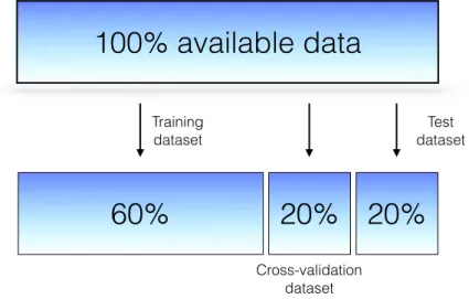
(30) CHAPTER 1. INTRODUCTION price of houses. For this example a house seller wants to know the estimated price of a new house according to its size in square meters. In order to know the estimated price of a new house we perform a linear regression using di↵erent models. We will use here a linear, a quadratic and a degree-6 polynomial function. The dataset is shown in Figure 1.3 as crosses and the continuous lines represent the best fit of each model.. Figure 1.3: Linear regression for polynomial models. On the top of each panel, the value of d shows the degree of the polynomial. The data is represented as crosses and is the same in each plot. Continuous lines represent the best fit for each model.. In this figure we notice that a linear model is not the best option for the prediction. This model under-fits the data meaning that the model is too simple. In machine learning vocabulary this is known as a high bias problem. The model itself is biased and this is reflected as a poor fit of the data. At the other extreme is the degree-6 polynomial function exhibiting a very accurate fit. This model touches each sample fitting the data perfectly and causing a problem known as overfitting. Thus, this is not a good feature of the model since it lacks the ability to generalize to new samples. This problem is known as high variance. The middle panel seems to be the mid-point between these two types of problems. One may wonder how to recognize these problems and the mid-point where a model can perform best. To quantitatively identify bias and variance and therefore optimize parameters we need to go through a process called crossvalidation. 1.2.2 Cross-validation In the previous section we recognized the problem of high variance (overfitting) in a dataset. This set of data is known as the training data because it was the data used by the model to build the estimator. If we now compute the error rate of 12.

(31) 1.2. DIAGNOSING LEARNING ALGORITHMS the overfit model, i.e. the degree-6 polynomial function, we will get zero error. However if we want to know the price of a new house using panel c of Fig. 1.3, the new price can be very di↵erent of the rest of the dataset. Therefore the training error is not a good indicator of the performance. To avoid this problem, the dataset should be divided into three smaller datasets that we will call: the training dataset, the cross-validation dataset and the test dataset, see Figure 1.4.. 100% available data Training dataset. 60%. Test dataset. 20% 20% Cross-validation dataset. Figure 1.4: Scheme of a possible data partitioning to avoid optimistic results.. The reason to split the data into three datasets come from the fact that we can overfit the data at di↵erent levels. The model parameters are learned using the training data. In our example, these parameters are the coefficients of the polynomial function. Once the model is trained, we evaluate the error using the cross-validation dataset and we choose the meta parameters, i.e. the degree of the polynomial function. As with the training, we could be overfitting the data respect to the meta parameters, thus the minimal cross-validation error tends to under-estimate the expected error on a new set of data. Then, the test dataset is the only one that the model has not seen and is the one used to evaluate the final model. Note that the test dataset is not used to optimize any parameter of the model but to evaluate its performance once all parameters are fixed. By partitioning the available data into three di↵erent sets, we drastically reduce the number of samples which can be use for training the model. However, the results can depend on a particular random choice for a pair of (train, validation) dataset. A solution to this problem is the basic approach of cross-validation (CV), known as k-fold CV where the training set is split into k smaller sets. The procedure is as follows: 1. The learning algorithm is trained using k. 1 folds, 13.

(32) CHAPTER 1. INTRODUCTION 2. then, the resulting model is evaluated using the rest of the data.. 3. The process is repeated by taking out a di↵erent fold of the k folds for the testing.. The performance of the k-fold CV is the average of the performance measure computed in the loop. This approach can be computationally expensive, but does not waste much data. There are other approaches to CV, however they follow the same principles. For example Leave-One-Out (LOO) is a simple cross-validation where each learning set is created by taking all the samples except one, the test set being the sample left out. Thus, for n samples, we have n di↵erent training sets and n di↵erent tests set. This cross-validation procedure does not waste much data as only one sample is removed from the training set. When we compare LOO with k-fold CV, one builds n models from n samples instead of k models, where n > k. (k 1)n Moreover, each model is trained on n 1 samples rather than k . In both ways, assuming that k is not too large and k < n, LOO is computationally more expensive than k-fold cross-validation. A version of leave-one-out CV is the leave-p-out CV that creates all the possible training-testing datasets by removing p samples from the complete set. With a cross-validation method, we can now choose the complexity of our model. Bringing back the example of the house seller from the previous section, the 20-fold cross-validation error of our polynomial classifier can be plotted as a function of the polynomial degree d. Figure 1.5 shows the reason why crossvalidation is important. On the left side of the plot, we have very low-degree polynomial, which under-fits the data. This leads to a very high error for both the training set and the cross-validation set. On the far right side of the plot, we have a very high degree polynomial, which over-fits the data. This can be seen in the fact that the training error is very low, while the cross-validation error is very high. Choosing d = 6 in this case gets very close to the optimal error. It might seem that something is amiss here: in Figure 1.5, d = 6 gives good results, but in Figure 1.3, we found that d = 6 vastly overfits the data. The di↵erence is the number of training points used. For Figure 1.3, there were only eight training points. In contrast for Figure 1.5, we have 100. As a general rule of thumb, the more training points used we use, the more complicated the model can be. But how can we determine for a given model whether more training points will be helpful? A useful diagnostic tool for this are the so called learning curves. 14.

(33) 1.2. DIAGNOSING LEARNING ALGORITHMS. Figure 1.5: Model complexity. This figure shows the 20-fold cross-validation error (blue line) and the training error (green line) as a function of the polynomial degree d of the model. For low degree, the system su↵ers high bias problem. In contrast, for high degree the model su↵ers high variance problem. The horizontal dashed line serves as a guide to a possible intrinsic error.. 1.2.3 Learning curves A learning curve is a graphical representation of the increase in learning as a function of experience. The concept was first used in psychology of learning by Ebbinghaus in 1885 [19, 20], although the name was not used until 1909. The plot of a learning curve depicts improvement in performance on the vertical axis when there are changes in another parameter (on the horizontal axis), such as training set size (in machine learning) or iteration/time (in both machine and biological learning). Then in machine learning, a typical learning curve shows training and cross-validation (CV) error as a function of the number of training samples. Note that when we train with a small subset of the training data, the training error is computed using this subset, not the full training set. These plots can give a quantitative view into how beneficial will be to add training samples. Let us describe what is happening and how to interpret a learning curve. Regarding the training error, when the number of samples is one or very small, any model (linear or nonlinear) can fit the data (almost) perfectly. This fact causes the training error to be zero or very small. As the number of samples in the training 15.

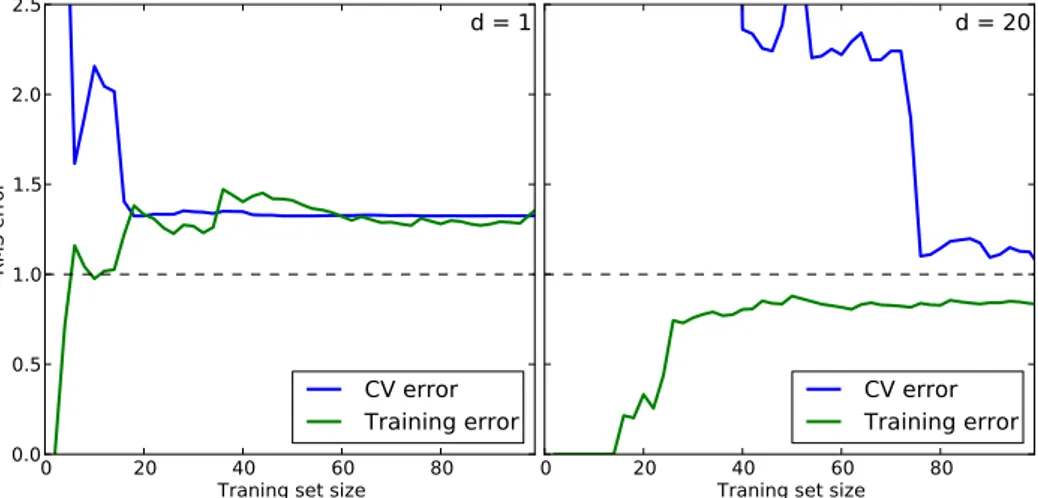
(34) CHAPTER 1. INTRODUCTION. error. cross-validation error. training error. number of samples. Figure 1.6: Typical learning curve.. set increases it becomes more difficult to fit all the points in the training set raising the training error. Eventually the training error will flatten once the number of training samples is enough to learn the patterns in the training dataset. In contrast, the cross-validation error is expected to be big for small number of samples because the parameters of the model are very inaccurate (they were trained using only one or few samples). As the number of samples increases, the parameter set of the model gets more accurate and the cross-validation error decreases until it flattens as the training error does. Figure 1.6 shows the expected shape of a learning curve. For small number of samples, the training error is minimal while the cross-validation error is maximal. As the number of samples in the training set increases, the two errors tend to flatten at a certain value that is determined by the task and the bias and variance of the model. To elaborate this last point, we come back to our example of the house seller. In Figure 1.5 we showed that using a hundred samples, a linear model shows high bias (underfitting) problems. In the learning curve this problem is recognized because the training and cross-validation errors converge very rapidly at a relative high error. We can see this behavior in the left panel of Figure 1.7. If we continue adding samples to the training set, it is unlikely that the situation changes. The two errors have converge to a certain value and they become independent of the number of samples. In the right panel of the same figure, we have the opposite case, a high variance problem given by a degree-20 polynomial model. The characteristic features of high variance (overfitting) is the gap that exists between the training and the cross-validation errors. If we increase the number of training samples it is likely that the gap reduces causing the errors to converge in the middle point. 16.

(35) 1.2. DIAGNOSING LEARNING ALGORITHMS. Figure 1.7: Learning curves depicting high bias (left panel) and high variance (right panel).. Small note about floating-point precision of a machine The theory of machine learning is based on statistics and basic mathematical operations and most of them can be explicitly solved. However, in practice we usually end up performing those operations using a computer. But there are limitations that we have to be aware of when using a numerical algorithm. For a training set with N samples, if N  d, being d the degrees of freedom of a model, the system of equations is perfectly solvable. This means that we can expect to have a perfect fit (zero error) between the data and the predicted model. The right panel of Figure 1.7 shows a degree-20 polynomial function. For N  20 the model should be solved exactly, however we can see non-zero errors before we reach the number of degrees of freedom of the model. This does not mean that the figure is wrong, in fact, the resulting fit has small residuals because it needs very large oscillations to fit all the points perfectly, similar to d = 6 case in Figure 1.3.. 1.2.4 Course to follow for high bias or high variance problems We have seen in this section that there are several tools to diagnose a learning algorithm. All these tools can be applied to the particular case of reservoir computing in order to evaluate, diagnose and improve performance. Here we present some actions that can be taken when a high bias or a high variance problem is found. When having high bias problems, we can: 17.

(36) CHAPTER 1. INTRODUCTION • Add more features. In our example of predicting house prices, including not only the size of the house but the year it was built, the neighborhood, and other features may help to a high-biased estimator. • Increase the complexity of the model. As we studied in section 1.2.1, for polynomial models we can increase the degree of the polynomial function to add complexity. Other kind of models will have their own methods for adding complexity. • Decrease regularization. Regularization is a technique used to impose simplicity in some machine learning models by adding a penalty term that depends on the characteristics of the parameters. If a model has high bias, decreasing the e↵ect of regularization can lead to better results. Refer to Section 1.1.2 for more information. • Use a smaller training set. This is more an advice than a guidance. Reducing the number of training samples will probably not improve the performance of the estimator since a high-biased model will keep the same error for smaller training datasets. However, for computationally expensive algorithms, reducing the training set can lead to improvements in computational speed. In contrast, if an algorithm is su↵ering a high variance problem, some steps we can follow are: • Use fewer features. Using a feature selection method may decrease the overfitting of the estimator. • Increase the training set. Adding samples can help to reduce a high variance problem as mentioned in section 1.2.3. • Increase regularization. Increasing the influence of the regularization parameter on the model may help to reduce overfitting. This term is intended to avoid exactly this problem. See Section 1.1.2. Up to this point of this thesis we have studied how to teach a learning algorithm such as artificial neural network or reservoir computing, to perform a task. We have also seen what we can do to optimize and diagnose problems in our model. We may wonder now how to quantify the goodness of a model, and how its performance is compared to other approaches. In the following section, we explore di↵erent measures to compare a model. 18.

(37) 1.3. EVALUATION OF PERFORMANCE 1.3. Evaluation of performance There are many measures of performance that have been traditionally used in machine learning. None of them being the measure that correctly shows how good or bad a model performs. These measures highlight the goodness or badness of some of model’s features. In this section, we introduce and discuss the pros and cons of some of the available measures of performance. This is not an exhaustive list since each kind of problem may have a particular set of measures that fits better for its evaluation. For example, measuring the performance of a time series estimator will use a di↵erent set of measurements than evaluating a classification algorithm. We will now describe measurements commonly used for classification tasks. Most of these measurements are based in a statistical tool named contingency table that can display the uni- or multi-variate frequency distribution of the variables. In machine learning this table is known as error matrix or confusion matrix. The latter will be the preferred term used in this thesis and it comes from the fact that this matrix makes it easy to recognize if a model is confusing two classes. 1.3.1 Confusion matrix In a classification task, a confusion matrix is a square matrix that allows to visualize the performance of an algorithm. In supervised learning we know the true labels of the test data, so a model has to estimate to which class each test sample belongs to. Having these two sets of labels, the real labels and the estimated ones, we can build a matrix that in its columns contains the estimation of the model while in the rows it has the ground truth. Figure 1.8 depicts a confusion matrix. To understand how it works, let us consider a 2-class classification task. One of the classes will be named the positive class, while the other the negative class. In a confusion matrix when a positive sample is classified by a model as such, it is counted as a True Positive (TP). In contrast, if the same sample is classified as negative then we have a False Negative (FN). A similar reasoning applies for a negative sample. If classified as positive, it is a False Positive (FP), and if classified as negative, it becomes a True Negative (TN). As a mnemonic technique we can read these terms using: it is ____ that is ____, i.e. a false negative can be read as "it is false that is negative", meaning that the real class of that sample is the positive class. False positive and false negative are, respectively, what we call type I and type II errors in statistical test theory. 19.

(38) CHAPTER 1. INTRODUCTION. Real values. Predicted values. positive. positive. negative. True positive. False negative (Type II error). negative. False positive (Type I error). True negative. Figure 1.8: Confusion matrix for a binary classification task.. Thus, from a confusion matrix we can derive a set of measurements that take into account di↵erent aspects of a classifier. Let us study some of these measures in the following sections.. Sensitivity Sensitivity (Se), also known as recall or true positive rate (TPR), represents the proportion of real positive cases correctly classified as positive. It is defined as. Se =. true positive ⇥ 100. true positive + f alse negative. (1.5). To give some intuition about the meaning of sensitivity, let us consider a population of subjects. Some of them are infected with a virus, and the rest are completely healthy. Imagine that a company designs a blood test to identify the infected subjects. The new blood test may report a sensitivity of 100% meaning that all infected subjects are correctly identified. If the test has zero sensitivity, it means it is unable to recognize any infected subject. This measure is very important in medicine because it allows to correctly identify medical conditions in patients. However it has to be taken carefully: If the test identifies not only all infected subjects but also some (or even all) of the healthy subjects as infected it will still report 100% sensitivity. This is because sensitivity accounts for the positive cases disregarding the errors of classifying a healthy subject as infected, i.e. the false positive cases. Then another measure is needed to quantify those healthy subjects incorrectly classified as infected. 20.

(39) 1.3. EVALUATION OF PERFORMANCE Precision Precision (Prec) or confidence denotes the proportion of predicted positive cases that are actually real positives. It can be expressed as Prec =. true positive ⇥ 100. f alse positive + true positive. (1.6). This measure solves the problem of misclassifying healthy subjects as infected. It complements sensitivity in the characterization of a classifier. So, a test report should at least show two performance measures to be meaningful. Note that precision still su↵ers the same drawback as sensitivity. It does not take into account those infected subjects that were not detected by the test, i.e. the false negatives. Specificity Specificity (Sp), also known as inverse sensitivity, inverse recall or true negative rate (TNR), is the proportion of real negative cases that are correctly classified. Specificity can be written as Sp =. true negative ⇥ 100. f alse positive + true negative. (1.7). Intuitively, if all the healthy subjects are correctly classified as not infected, the blood test will have specificity of 100%. Note that if some (or all) of the infected subjects are classified as healthy, the blood test still will be a 100% specific. There is a complementary measure from specificity called False Postive Rate (FPR) that is defined as FPR =. f alse positive . f alse positive + true negative. (1.8). Accuracy Accuracy (Acc) is the combination of the previous mentioned measures. It is defined as, true positive + true negative Acc = , (1.9) sum o f all samples It can be seen as a weighted average between sensitivity and specificity [21]. Sensitivity and specificity are linked such that changing the sensitivity a↵ects the specificity of a test. In the following sections we will describe how they interact. 21.

(40) CHAPTER 1. INTRODUCTION 1.3.2 The trade-off between sensitivity and specificity We will illustrate the trade-o↵ between these measures using an example. We have again a blood test to discriminate healthy from infected subjects. Imagine that the result of the test is a counter, such as the concentration of a certain substance in a certain volume of blood. We decide to evaluate the test over a population that is healthy. Thus we are going to have a certain distribution of test values for those healthy subjects. If we now perform the test over an infected population, we will then have the corresponding distribution of test values for infected subjects. Figure 1.9 depicts this situation.. Frequency. Threshold. Healthy subjects. 25. Infected subjects. 50. 75. Test value. Figure 1.9: Distribution of test results in a healthy (blue) and infected (red) population.. Let us say that small concentrations of our substance is a healthy indicator, and a high concentration means infection. Now, the problem we are facing is to decide from up to which point the test is going to be considered negative and from which point it is going to be considered positive. This can be done by setting a threshold value that separates the two distributions. In this example, it looks natural to set that threshold at a value of 50 since our two distributions do not overlap. Now consider a more interesting scenario where the two distributions overlap, as shown in Figure 1.10. For this case, setting a threshold is a more difficult task. To begin with, let us keep the threshold in the middle, as we did in the previous figure. Now, to identify the true/false positive/negative values in this scheme we consider one distribution curve at a time. We start considering only the distribution of the infected subjects. On the right of the threshold line are those concentrations that we consider positive and come from infected subjects, so these are true positives (TP). On the left of the threshold line are those concentrations that we consider negative (because they are in the left side of the 22.

(41) 1.3. EVALUATION OF PERFORMANCE division line) but are actually positive, i.e. they are in the positive distribution curve. Then these cases represent the false negatives (FN). If we now consider the distribution for the healthy subjects, we can identify the true negatives (TN) as those concentrations in the left of the threshold line and as false positives (FP) those on the right of the threshold line.. Frequency. Threshold. Healthy subjects. Infected subjects. TN. TP. FN FP. 25. 50. 75. Test value. Figure 1.10: Overlapping distribution of test results in a healthy (blue) and infected (red) population.. So sensitivity is the proportion of the area under the positive distribution curve that is at the right of the threshold line with respect to the area under the full positive distribution curve. Note that if we move the threshold line to the left, the sensitivity will increase but it also will include more false positives. In the extreme case, if we set the threshold line all the way to the left, we will get a 100% sensitivity but our test will lack the ability to distinguish healthy from infected subjects, i.e. it will classify every subject as infected. On the opposite side, specificity is the proportion of the area under the negative distribution curve to the left of the threshold line with respect to the area under the full negative distribution curve. Again, we can increase this proportion by setting the threshold line to the right. However this will increase the amount of false negatives. A similar relationship between sensitivity and precision, or any confusion matrix derived measure can be established. In conclusion, one has to set a threshold value for a given test in order to characterize it. This threshold value is going to define the sensitivity and specificity of the test. There is no general rule to choose this threshold. It depends on the task and the peculiarities of the estimator. One way to visualize the general properties of an estimator using the above mentioned trade-o↵ is the so-called receiver operating characteristics (ROC) curve. 23.

(42) CHAPTER 1. INTRODUCTION 1.3.3 Receiver operating characteristics curve A Receiver Operating Characteristics (ROC) curve is a statistical tool to visualize the performance of a classifier when the threshold that defines the classes is varied. It is based on the trade-o↵ between sensitivity and specificity (section 1.3.2). To build a ROC curve, we need to plot the sensitivity of the classifier as a function of the false positive rate (FPR, shown in equation 1.8) for di↵erent values of the discriminating threshold.. Figure 1.11: A ROC curve with the line of nondiscrimination. Each step in the curve corresponds to a value of the threshold that separates one class from the other. Image by [18].. Figure 1.11 depicts the ROC space. The best classifier will have coordinates (0, 1), representing a 100% sensitivity and a 100% specificity. This point is also called perfect classification. Departing from this point, the performance of our classifier describes a curve. The identity line, a straight line that connects the (0,0) point with the (1,1) point, is called the line of nondiscrimination and represents a random guess. Curves above this line are considered to exploit information from the data for a good classification. Curves overlapping the line of nondiscrimination do not contain information about the classes and make the classification randomly. Any curve under this line performs worse than a random classifier. In this case, the classifier contains information about the classes but it uses this information incorrectly [22]. Another good property of ROC curves is that they are insensitive to changes in class distribution (class skew) [23], i.e. they do not depend on the number of instances in each class (data balance). 24.

(43) 1.4. OBJECT OF THE RESEARCH WORK Area under a ROC curve ROC curves provide a lot of information for characterizing classifiers. However one can reduce this information in order to give an overall measure of performance. A common quantity that fulfills this criterion is the so-called Area Under the Curve (AUC) [24]. A property of ROC curves is that they are drawn in a unitary square, so that the AUC ranges from 0 to 1. If the AUC of a classifier is less than 0.5, it is said that the classifier is unrealistic [23]. If the AUC is 1, it represents the perfect classifier. From this, we could say that the higher the AUC the better the classifier. In the example ROC curve in Figure 1.11 the AUC = 0.79. The AUC should be used to summarize the information on a ROC curve but it should not substitute it since there are classifiers with high AUC that can perform worse in a specific region of the ROC space than a classifier with low AUC [23].. 1.4. Object of the research work The object of this thesis is the study of the computational properties of delaycoupled systems and their applications. To this end, several tasks are tackled: 1. Build a computational toolbox for the numerical study of delay-coupled systems. 2. Implement a delay-based reservoir computer for the study of the computational properties that are intrinsic to this kind of system and are independent of the task to be performed. 3. Describe the working principles of a reservoir computer by studying typical machine learning tasks that are difficult to solve by using conventional computing. 4. Apply the computational power of delay-coupled systems to a real-world open biomedical problem. 5. Study the influence on performance of multivariate inputs in a reservoir computer. 6. Development of a computational framework that allows the tuning of a hardware implementation based on a semiconductor laser dynamics. The di↵erent parts of our main objectives are developed along this manuscript. A description of the structure of this research work is given in the next section. 25.

(44) CHAPTER 1. INTRODUCTION 1.5. Structure of this thesis. This thesis is based on the research developed at the Instituto de Física Interdisciplinar y Sistemas Complejos (IFISC) during the period 2011-2015. The results of the di↵erent studies have been published in several international recognized scientific journals. The related articles are enumerated in the List of Publications. This manuscript is divided in three parts. The first part called Introduction is composed of one chapter, Chapter 1, and gives an overview of machine learning by focusing on a particular kernel type known as reservoir computing. Standard methods for the diagnostics and evaluation of learning algorithms are introduced in this part. The second part, called Methodology, results and discussion contains the core of this thesis. It is composed of 4 chapters. The first one, Chapter 2, describes the principles of information processing using delay-coupled systems. This chapter describes the computational properties of the delay-coupled approach. After this description, results are presented using the proposed scheme for reservoir computing, tackling typical machine learning tasks, such as a classification task (spoken digit recognition), a time-series estimation task and a modeling task. Each task’s section is self-contained, including its description, aim of the task, results and discussion. In this way, the reader might jump among the di↵erent tasks without getting lost. The end of this chapter, presents a short exploration of the reservoir’s performance in di↵erent conditions other than the typical ones. In particular, the spoken digit recognition task is used in the evaluation of performance of the reservoir with di↵erent initial conditions. An evaluation of the performance when reading out a portion of the dynamical states of the system, i.e. reading some virtual nodes, is also presented. The evaluation of a especially designed reservoir computer for the application in a medical task is presented in Chapter 3. This chapter contains a brief description of the physiology of the cardiovascular system and, in particular, of the heart. The reservoir computer utilizes electrocardiographic signals for the classification of cardiac arrhythmias. The origin of these signals and how they are prepared to be included in our designed computer is described. A particular feature of our approach is the learning method. We exploit the statistical properties of the logistic regression method. This learning procedure is particularly suitable in biostatistical tasks were binary solutions are expected, such as normal or abnormal heartbeat. Results in internationally recognized format for the evaluation of arrhythmia classifiers and for clinically relevant scenarios are presented and discussed at the end of this chapter. 26.

(45) 1.5. STRUCTURE OF THIS THESIS The computational power found in the delay-coupled system described in the previous chapters is evaluated using multivariate inputs in Chapter 4. Two tasks are utilized to demonstrate that a reservoir computer might utilize beneficially information from di↵erent variables of the system under study. We use as examples: a time-series estimation task based on the Lorenz system in a chaotic regime and the classification task presented in Chapter 3 when using two electrocardiographic signals recorded simultaneously from di↵erent sites of the chest. Numerical implementations of the reservoir computer described in this thesis might be implemented in hardware using optical nonlinearities. Chapter 5 describes the numerical implementations of a semiconductor laser serving as the nonlinear node of a reservoir computer. This chapter shows the expected performance of such reservoir under di↵erent conditions allowing to tune specific parameters for a hardware implementation. Only numerical computations are shown in this chapter. The interested reader in the hardware implementation is refer to the corresponding article [25] and references there in. The final part of this thesis is Conclusions part. It is composed of one chapter, Chapter 6. In this part we summarize what we have accomplished along the di↵erent parts of this research work. We also present some potential changes in the proposed scheme that we believe are important to understand might be useful for future applications. At the end of the manuscript, an appendix related with technical descriptions of the electrocardiographic database is presented. Also, a small glossary and a list of the acronyms used in this thesis are described. The bibliography can be found at the very end of this thesis, showing references in order of appearance.. 27.

(46)

(47) Part II Methodology, results and discussion. 29.

(48)