Disentangling the Galactic Halo with APOGEE II Chemical and Star Formation Histories for the Two Distinct Populations

(1)

Disentangling the Galactic Halo with APOGEE. II. Chemical and Star Formation

Histories for the Two Distinct Populations

Emma Fernández-Alvar1, Leticia Carigi1, William J. Schuster2, Christian R. Hayes3, Nancy Ávila-Vergara1,4, Steve R. Majewski3 , Carlos Allende Prieto5,6 , Timothy C. Beers7 , Sebastián F. Sánchez1 , Olga Zamora5,6,

Domingo Aníbal García-Hernández5,6, Baitian Tang8 , José G. Fernández-Trincado8,9, Patricia Tissera10 , Douglas Geisler8 , and Sandro Villanova8

1_{Instituto de Astronomía, Universidad Nacional Autónoma de México, AP 70-264, 04510, Ciudad de México, México} 2

Instituto de Astronomía, Universidad Nacional Autónoma de México, AP 106, 22800 Ensenada, B. C., México

3

Department of Astronomy, University of Virginia, Charlottesville, VA 22904-4325, USA

4

Departamento de Física y Matemáticas, Universidad Iberoamericana, Prolongación Paseo de la Reforma 880, Lomas de Santa Fe, CP 01210 México DF, México

5

Instituto de Astrofísica de Canarias, Vía Láctea, E-38205 La Laguna, Tenerife, Spain

6

Universidad de La Laguna, Departamento de Astrofísica, E-38206 La Laguna, Tenerife, Spain

7

Department of Physics and JINA Center for the Evolution of the Elements, University of Notre Dame, Notre Dame, IN 46556, USA

8

Departamento de Astronomía, Casilla 160-CUniversidad de Concepción, Concepción, Chile

9

Institut Utinam, CNRS UMR6213, Univ. Bourgogne Franche-Comté, OSU THETA , Observatoire de Besançon, BP 1615, F-25010 Besançon Cedex, France

10

Departamento de Ciencias Físicas, Universidad Andres Bello, Av. Republica 220, Santiago, Chile Received 2017 August 3; revised 2017 September 29; accepted 2017 October 15; published 2018 January 5

Abstract

The formation processes that led to the current Galactic stellar halo are still under debate. Previous studies have provided evidence for different stellar populations in terms of elemental abundances and kinematics, pointing to different chemical and star formation histories(SFHs). In the present work, we explore, over a broader range in metallicity (-2.2<[Fe H]< +0.5), the two stellar populations detected in the ﬁrst paper of this series from metal-poor stars in DR13 of the Apache Point Observatory Galactic Evolution Experiment(APOGEE). We aim to infer signatures of the initial mass function (IMF) and the SFH from the two α-to-iron versus iron abundance chemical trends for the most APOGEE-reliableα-elements(O, Mg, Si, and Ca). Using simple chemical-evolution models, we infer the upper mass limit (Mup)for the IMF and the star formation rate, and its duration for each population. Compared with the low-α population, we obtain a more intense and longer-lived SFH, and a top-heavier IMF for the high-α population.

Key words:Galaxy: evolution– Galaxy: halo– stars: abundances

Supporting material:machine-readable table

1. Introduction

Theﬁrst indications concerning a dual(or multiple)Galactic halo arose from the confrontation between the scenario of Eggen et al.(1962,ELS)and that of Searle & Zinn(1978,SZ). On one hand, we have the monolithic collapse, or free-fall, model of ELS, derived from various orbital-parameter versus ultraviolet-excess diagrams for 221 “well-observed” dwarf stars, which showed correlations suggesting a nearly free-fall collapse. On the other hand, we have the infall of“protogalactic fragments” proposed by SZ from the differences in the composition found between inner- and outer-halo globular clusters. Several reviews presented the strengths, weaknesses, and similarities of these two scenarios, such as Sandage(1986), Gilmore et al.(1989), and Majewski(1993).

It was suggested by some authors that these two contrasting views of halo formation were related to differences in the tracers themselves, halo ﬁeld stars compared to globular clusters, or bias arising from their proper-motion-based selection (Mihalas & Binney1981; Yoshii1982; Norris et al.

1985; Chiba & Beers2000). However, later studies using rele-vant observations discussed the implications and importance of combining such ideas in a dual-halo model for the Galaxy (Zinn 1993). For example, evidence for two Galactic halo components was found (Márquez & Schuster 1994; Carollo et al.2007,2010; Marín-Franch et al.2009; de Jong et al.2010; Jofré & Weiss 2011; Beers et al. 2012), using uvby–β

photometry of haloﬁeld stars, globular clusters, and data from the Sloan Digital Sky Survey(SDSS; York et al.2000)and the sub-program Sloan Extension for Galactic Understanding and Exploration (SEGUE; Yanny et al. 2009) and its extension, SEGUE-2.

Other studies revealed an even more complicated scheme for the Galactic stellar halo, with the discovery of streams, shells, clumps, tidal tails, debris, and the presence of correlated substructures of halo stars(e.g., Schlaufman et al.2009,2011,

2012; Carlberg et al.2012; Koposov et al.2012; Duffau et al.

2014; Slater et al.2014; Carlin et al.2016), pointing to a more chaotic dual, or even triple, component halo system (see Morrison et al. 2009), extrapolating beyond the ideas of SZ. Reviews concerning such observations and substructures for the stellar halo are given in Helmi (2008), De Lucia (2012), Belokurov et al.(2014), and Bernard et al.(2016).

(2)

measured in presently observed stellar atmospheres provides information about the properties of the previous stellar populations, such as the initial mass function (IMF) or the star formation rate (SFR)at early times—see Figure1. These properties also allow us to constrain the processes that our Galaxy underwent during its early assembly.

Signatures of a dichotomy in theα-to-iron ratios in halo stars were detected (Nissen & Schuster 1997; Fulbright 2002; Gratton et al.2003; Ishigaki et al.2013), related in some cases to the distance from the Galactic center (Ishigaki et al.2010). Then, in a series of papers, Nissen & Schuster (2010,2011—

hereafterNS10,NS11; and Schuster et al.2012)obtained high-precision (±0.01–0.04 dex) relative abundance ratios for 94 dwarf stars over the metallicity range−1.6<[Fe/H]<−0.4, with 78 having halo kinematics according to the Toomre diagram, plus 16 thick-disk stars. Two groupings were clearly found in diagrams such as [Mg/Fe]versus [Fe/H] or [α/Fe] versus[Fe/H], with 56 high-αhalo and thick-disk stars falling together, along with 38 low-αhalo stars in the sample.

Clear separations between these two halo components were found for the elements Mg, Si, Ca, Ti, Na, Ni, Cu, and Zn with respect to iron, and also for[Ba/Y], all as a function of[Fe/H] (Ramírez et al. 2012 conﬁrmed the same for [O/Fe]). In Schuster et al.(2012), it was shown that the high-α halo stars have ages higher by 2–3 Gyr than the low-α ones, and also smaller average values for the orbital parametersrmax,zmax, and emax. Again, some concordance with the ideas of ELS plus SZ were found (for example, via the in situ and accreted stellar populations of Zolotov et al. 2009, 2010; see also Tissera et al.2013).

We should note that the distinction between two populations of stars for high[α/Fe]versus[Fe/H]has also been observed in between the thick and thin disk(Hayden et al.2015), and also in other galaxies different than the Milky Way. Recently, Walcher et al. (2015)demostrated that early type galaxies present these two populations, associated with older (alpha-enhanced) and

Evolution Experiment (APOGEE; Majewski et al. 2017; Nidever et al. 2015), is gathering high-resolution, high signal-to-noise near-IR spectra to map the principal compo-nents of the Milky Way. With, eventually, a half million spectra, the APOGEE database is a very valuable sample to check previousﬁndings, and to more completely investigate the chemical properties of stellar populations. Recently, investiga-tions of metal-poor stars in the APOGEE database have shown signatures of the two chemically distinct populations revealed by Nissen & Schuster(Hawkins et al.2015; Hayes et al.2017, hereafter Paper I).

Encouraged by the possibilities of a chemical analysis of the two halo populations discovered in the APOGEE database, we aim to obtain information on the IMF, stellar yields, and SFH, or equivalently, SFR versus time, from the DR13 (Albareti et al.2017)chemical abundances provided by APOGEE. This paper is organized as follows. The sample selection is discussed in Section 2. Section 3 describes the split of the sample into two populations, the derivation of the corresp-onding chemical trends, and the theoretical model from which we infer properties for each population. In Section4, we relate our main results, and we discuss them in Section5. Section6

summarizes our conclusions.

2. Sample

APOGEE is an SDSS program (Eisenstein et al. 2011; Blanton et al.2017)conceived to explore the structure of the Milky Way. The ﬁrst APOGEE phase was in SDSS-III and collected data between 2011 and 2014 July, obtaining high-resolution (R∼22,500)spectra with a typical signal-to-noise

100 using a multiobject infrared spectrograph coupled to the 2.5 m SDSS telescope at the Apache Point Observatory(Gunn et al.2006; Wilson et al.2010). The targets map the Galactic disk, bulge, and halo (Zasowski et al. 2013). More than 143,000 objects were observed as part of that program.

The APOGEE Stellar Parameters and Abundances pipeline (ASPCAP) was developed to obtain stellar atmospheric parameters and chemical abundances from the H-band (1.5–1.7μm), the spectral range covered by the APOGEE spectrograph. The methodology is based on the comparison with synthetic spectra in an N-dimensional parameter space, looking for the best ﬁt with observations (more details in García Pérez et al. 2016). Abundances with accuracies ∼0.1 dex have been derived, and radial velocities have been determined with accuracies of ∼0.1 km s−1 (Holtzman et al.

2015). DR12 (Alam et al. 2015)was the ﬁnal SDSS-III data

Figure 1.Scheme that we use to identify the chemical trends observed in the

[Mg/Fe]vs.[Fe/H](and otherα-elements)for our sample(see Figures2and

(3)

release. The thirteenth data release(DR13; Albareti et al.2017)

provides the ﬁnal products of a reanalysis, after including several improvements to the pipeline. Chemical abundances of up to 26 chemical species are available for some stars, including theα-elements: O, Mg, S, Si, Ca, and Ti.

From this database, we want to draw a sample of halo stars. These objects clearly exhibit different kinematics from disk stars; objects with large heliocentric radial velocities have a high probability of belonging to this Galactic component.

In addition, the l-GRV cos( )b space(GRV is the radial velocity vrad corrected for solar motion,

11

and l and b are the galactic longitude and latitude)can be used to isolate halo stars from disk stars. As performed by Hawkins et al.(2015)for the same purpose, we exclude from our sample those stars following a sinusoid of amplitude corresponding to the rotational velocity of the disk in the solar circle (220 km s−1; Schönrich 2012) and a dispersion more than three times the dispersion of the same curve deﬁned by disk stars.

This is the sinusoid expected to be drawn by objects rotating in the Galactic plane. Halo stars occupy randomly the GRV/ cos(b) versus l space and, consequently, this selection criteria excludes not only disk stars but also stars belonging to the Galactic halo. However, we prefer to select only those objects with the highest conﬁdence to be halo stars, even if our selection criteria is quite restrictive.

This selection to exclude disk stars works best in the case of objects at ∣ ∣b <60 (Majewski et al. 2012). Therefore, we measured the dispersion for stars at ∣ ∣b <60, having

>

[Fe H] 0.0, which we expect to be dominated by disk stars. Thus, to explore stars with halo kinematics we select objects with vrad>180 km s−1 and/or stars at ∣ ∣b <60 with an absolute values of GRV/cos(b) more than three times larger than that measured with disk stars in bins of20inl.

The key to identifying different stellar populations by their chemistry is the accuracy and precision with which their chemical abundances are measured (Lindegren & Feltzing

2013). Both are also needed to infer parameters of the SFH from their chemical abundance trends. The random abundance uncertainties in the ASPCAP analysis vary as a function ofTeff

and [Fe/H], as illustrated in Figure 2 of Bertran de Lis et al. (2016). They evaluated the[O/Fe]uncertainty as a function of these parameters by measuring the scatter observed in clusters. In light of these results, we select stars in theTeffrange at which the precision in [O/Fe]is the highest for the metallicity range covered by our halo sample (−2.5<[Fe/H]<+0.5). We choose the interval 4000<Teff<4500K, where the[O/Fe]

uncertainties are σ[O/Fe]0.02 dex, for −0.6<[Fe/ H]<+0.2, and increasing at lower metallicities. The empirical uncertainties calculated by ASPCAP are, on average, d=0.05dex for [O/Fe] and [Mg/Fe], with a standard deviation s=0.03dex and 0.02 dex, respectively, and d=0.04dex and 0.07 dex with s=0.02dex and 0.06 dex, for[Si/Fe]and[Ca/Fe], respectively.

We exclude stars with distances(adopted using the techniques of the Brazilian Participation Group—BPG; Santiago et al.

2016) from the Galactic center r4 kpc, in order to avoid bulge stars. We know that this selection cut may also exclude some halo stars located at this range of distances. However, we want to avoid any possible bulge contamination due to our goal of characterizing only the halo component of our Galaxy.

Finally, we reject objects with ASPCAP flags possibly indicating poor estimates. We also reject targets in globular clusters in our Galaxy and in Andromeda—these show chemical abundances that strongly deviate from the chemical trends of field stars (Mészáros et al. 2015). Our sample is comprised of field stars. We do not expect to have included objects from dwarf spheroidal galaxies, because APOGEE only purposely targeted in DR13 the spheroidal Sagittarius. Most of their stars are cool M giants with Teff<4000K, and we

rejected them by ourTeff selection criteria.

Each star of our ﬁnal sample is assigned to belong to the Galactic halo merely based on its vrad. A more robust attribution will be possible with Gaia parallaxes and proper motions very soon.

Within theα-elements derived by ASPCAP, S and Ti are less reliable.[Ti/Fe] derived from both neutral and ionized atomic lines shows a large dispersion, and differing trends in the[Ti/Fe] versus [Fe/H] space. In their evaluation of the ASPCAP products, Holtzman et al.(2015)warned about the reliability for this element’s abundances. They found no trend of[Ti/Fe]with [Fe/H], which led them to suspect that some systematic error affected their measurement. [S/Fe] also exhibits a large dispersion. At low metallicities, the SI lines from which ASPCAP derives [S/Fe] abundances become weak and comparable to the noise level. The measured[S/Fe]abundances lead to enhanced values and are likely to be unreliable.

3. Methodology

Ourﬁnal sample comprises 175 stars. The 2MASS id as well as the main stellar atmospheric parameters and chemical abundances for the selected sample are shown in Table1. The top panel of Figure2shows the comparison between[Mg/Fe]as a function of[Fe/H]. Two different chemical trends are clearly distinguishable. We split the two stellar populations(High-Mg and Low-Mg)following the same classiﬁcation derived from the statistical analysis presented in Paper I from a larger sample, i.e., along[Mg/Fe]=−0.2[Fe/H]. In the bottom panel, we overplot the NS10 sample of halo stars with their[Mg/Fe]and [Fe/H] measurements. Their sample abundance trends follow very closely our results from APOGEE data.

We investigate these two populations in the[X/Fe] versus [Fe/H] space for the other APOGEE-reliable α-chemical species determined by ASPCAP. The chemical abundances and their errors are displayed in Figure 3 (for the High-Mg population, upper panels, and for the Low-Mg population, lower panels). In order to better visualize the chemical trends and the differences between the two populations, we calculate the weighted mean [X/Fe] and its statistical error in [Fe/H] bins of 0.1 dex, with a minimum ofﬁve objects per bin.

Figure 4 shows the [X/Fe] versus [Fe/H] for each population. The High-Mg population shows the largest enhancement of all theα-elements considered here. This broad separation is the reason we used this element as the primary discriminator of halo populations in Paper I. The enhancement level diminishes with O, Si, and Ca. For this reason, and to be consistent with the nomenclature in theﬁrst paper of this series, we refer to these populations as High-Mg (HMg) and Low-Mg(LMg).

The [X/Fe] versus [Fe/H] trends (see Figure 4) can be divided into two parts, as we depict in Figure1:

11

We adopt the solar Galactocentric velocities U=11.1km s−1, V=

(4)

1. The“thigh”: This corresponds to the semi-plateaulocated between the lowest metallicity ([Fe H]l ~ -1.9 and ~-1.4for the LMg and HMg populations, respectively)

and theknee([Fe H]k ~ -1.0and~-0.4for the LMg

and HMg populations, respectively). The[Fe H]k is the metallicity at which the downward slope becomes steepest.

2. The “shin”: located between the metallicity of theknee

and the largest metallicity,[Fe/H]h.

The chemical trends observed for the HMg and LMg sub-samples in each one of these metallicity ranges are the result of a different chemical and SFH for each stellar population, as explained below.

We use the calculated weighted means, choosing bins of different sizes to determine the mean[Fe/H]at which the slope of the trend changes, corresponding to the knee of the population. We identify the HMg knee at [Fe/H]∼−0.4, and the LMgkneeat[Fe/H]∼−1.

It is important to notice that not all the elemental abundances could be measured for every star. In some cases, it was not possible to determine the abundance of a particular element reliably due to the quality of the observations. For this reason, the number of stars in each sample slightly varies from one element to another, as well as the particular objects from which the means are calculated. This implies that the mean[Fe/H]l, [Fe/H]k, and[Fe/H]hfor each population are slightly different, depending on the chemical element that we consider. Table2

shows the resulting variousá[Fe H]ñfor each α-element. Due to the low number of stars, the weighted means have large errors, in particular, at low metallicities, and they do not describe smooth chemical trends. For this reason, we perform a linearﬁt to the weighted[X/Fe]means in the“thigh”and in the “shin”metallicity ranges; see Figure4.

3.1. Chemical-evolution Model

As mentioned in the Introduction, we aim to obtain basic chemical histories for the HMg and LMg populations. In

Figure 2.[Mg/Fe]as a function of[Fe/H]for our sample in both panels, with the NS10 sample overplot in the bottom panel. APOGEE data are shown as dots. Triangles represent the [Mg/Fe] values from NS10. The black dashed line separates the sample in two populations as in Paper I, along[Mg/Fe]=−0.2

[Fe/H]. We extrapolate the separation to lower[Fe/H]. The High-Mg population is shown with blue symbols, while the Low-Mg is shown with red symbols.

Figure 3.[X/Fe]as a function of[Fe/H]for the reliably ASPCAP measured chemical elements, O, Mg, Si, and Ca, with their associated errors for the HMg (top panels)and for the LMg(bottom panels)populations.

Figure 4.[X/Fe]as a function of[Fe/H]for theα-elements O, Mg, Si, and Ca in each panel. The populations are color-coded as in Figure2. The weighted mean[X/Fe], calculated in bins of 0.1 dex in[Fe/H](considering a minimum of 5 objects per bin), with their corresponding errors, are overplotted in blue and red for the HMg and LMg populations, respectively. Linearﬁts to the weighted[X/Fe]means are overlapping(blue and red solid lines). The six more metal-poor values resulting from theﬁt and use to infer the IMFMupare indicated with numbers in the left top panel corresponding to [O/Fe] vs.

(5)

particular, we try inferring the upper mass (Mup)of the IMF, the integrated yields for massive stars(Y), the fractions of Type II supernovae (SN II)and Type Ia supernovae(SN Ia) (fSN II and fSN Ia, respectively)in each simple stellar population, and the efﬁciency(ν)of the SFR and duration(th)of the SFH.

In order to obtain general properties for each population, our simple chemical-evolution models are built based on the following assumptions:

1. The HMg and LMg are two independent populations. Each population evolves in its own way, according to the trend described by the mean[X/Fe]values for O, Mg, Si, and Ca versus[Fe/H](See Figure4).

2. We embrace the semi-instantaneous recycling approx-imation. In this approximation, after each burst of star formation, all massive stars explode as SN II, instanta-neously enriching the ISM. SN Ia explode with a delay of about 1 Gyr after their progenitors are formed. For a similar prescription, see Franco & Carigi (2008) and Hernández-Martínez et al. (2011).

3. A closed-box model that evolves from initial primordial gas. We assume one zone per population, and a continuous SFH. These SN II behave similarly to the SN II in the “thigh.”

Based on assumptions 2 and 3, the chemical abundance by mass(X)of12an element in the ISM evolves between any two times,t1andt2(>t1)

whereYXis the synthesized mass fraction of element X ejected by dying stars, á ñYX 2 1- represents the Z-average integrated yields between Z t( )1 andZ t2( )(i.e.,Z t( )j =0.02´10[Fe H]j), m( )t =Mgas( )t Mgas( )0 is the gas consumption,Mgasrepresents the gas mass, and Mgas( )0 is the initial gas mass (see

Avila-Vergara et al. 2016).

For computing á ñYX, we consider theoretical Z-dependent

yields for SN II by Kobayashi et al.(2006)and for pre-SN by the Geneva group(see Robles-Valdez et al.2013). We integrate these yields in mass over a Kroupa–Tout–Gilmore IMF (Kroupa et al. 1993). The integrated yields are calculated between 0.1M and Mup, where Mup=10 to 40 in steps of

Equation (2) relates the abundance ratios (derived by ASPCAP from the observations) with the integrated yields (from theoretical yields and the IMF). For obtaining the best

Mup values that reproduce the data, we apply Equation(2)on the “thigh,” because during this range only SN II enrich the ISM.

Based on the data, we can obtain X/H (the fraction by number) from [X/Fe]−[Fe/H], taking into account the solar abundances by Asplund et al. (2005). These are the solar chemical abundances considered by ASPCAP in the generation of the synthetic spectra of the grids used to determined the elemental abundances from APOGEE spectra. We calculate X/H and Fe/H ratios from the values derived by the linearﬁt over the weighted[X/Fe]means shown in Figure4. Then, we transform the X/H value by number to X/H by mass.

3.1.1. The“Thigh”

We infer the Mup of the IMF for each population from the “thigh.” We use O abundances because, in the literature, chemical-evolution models cannot reproduce the [Mg/Fe]– [Fe/H]trend shown by stars of the solar vicinity. For example, according to Romano et al. (2010), Mg in halo stars is reproduced when models considered yields by Kobayashi et al. (2006) for supernovae and hypernovae, but with this yield combination Mg in disk stars does notﬁt, mainly in thick-disk stars.

Figure5 shows the theoretical log(YO YFe) versus Mup for stellar initial metallicities equal to 0.001, 0.004, and 0.02(cyan, magenta, and black lines). We add the yield ratios interpolated for the metallicities(Zj)that corresponds to the[Fe/H]means convenience, we focus on the X/Fe that show lower errors. From the intersection between the theoretical yields and the measured abundances we infer the Mup. The inferred Mup ranges are located between vertical dotted lines (for the high-and low-αpopulations, upper and bottom panels, respectively). Based on the mean Mup values corresponding to the inferred

Mupranges, we compute the fraction of SN II(

ò

M

8

up

IMF(m)dm)

for each simple stellar population and the integrated yields between8M andMup.

Considering that theoretical Fe yields for massive stars,

áY_Fetheo,IIñ, are well-computed and do not require correction, we employ Equation (2) to obtain the empirical yields,áY_Xemp,IIñ, needed to reproduce the observed [X/Fe] versus [Fe/H] between the fourth mean point and theknee, the most reliable range for the“thigh.”

each of the α-elements and populations, which are close to unity. Error bars are calculated from the minimum and maximum Mup (see Table 3) assumed in the computation ofáY_Fetheo,IIñ.

12

(6)

Oxygen presents the largest errors because O yields are the most stellar-Z and mass-dependent ones among the four APOGEE-reliable α-elements. The Mg correction factor is the most different between the populations, due to the high-Mg enhancement shown by the HMg population.

3.1.2. The“Shin”

Again, we apply Equation (2), but now for the “shin” (between the knee and the[Fe H]h), taking into account the same correction factors for integrated yields of massive stars (áY_Xemp,IIñ) obtained in the “thigh” range. As previously mentioned, SN II and SN Ia contribute during the “shin”to the ISM enrichment in alpha and Fe elements. Therefore

Z-average integrated yields (á ñYXk-h) between Z t( )k and Z t( )h are

á ñYXk h- = áYemp,IIñk h- +fSN Ia ´yX, ( )5 Ia

whereyXIais the SN Ia yield for a speciﬁc element, andfSN Iais the fraction of SN Ia that is contributed during the “shin.”In this range, the contribution of low- and intermediate-mass stars are not considered, either because these stars do not produce the α-elements considered in this paper, or their yields are negligible compare with the SN II and SN Ia yields.

Substitutingá ñYXk-h andáYFeñk-h in Equation(3), we obtain

fSN Ia. Figure7 shows thefSN Iavalues(upper panel)and f f

SN Ia

SN II

for each α-element and population. Figure 8 shows the percentage contribution of SN Ia and SN II to theα-element enrichment.

Finally, this basic model also allows us to estimate the efﬁciency of the SFR and the times when M Hk and M Hh occur. For that, in Equation(1), we assume the following:

1. The SFR is proportional to the Mgas, with efﬁciency ν,SFR( )t =nMgas( )t .

2. νis constant during the entire evolution. 3. tk=delay time‐ forSN Ia=1 Gyr, and

Figure 5.Comparison of the oxygen yield to iron yield ratio(YO YFe)with the

DO DFevalues(see Equation(3))for the HMg population(upper panel)and the LMg population(lower panel). Inclined continuous lines:YO YFe, results of

integrating IMF-weighted-yields from 8MetoMup(10, 15, 20, 25, and 30Me)

for different initial stellar metallicities. Inclined thick lines:YO YFe for the

initial metallicities (0.001, 0.004, and 0.02; cyan, magenta, and black) considered by Kobayashi et al. (2006). Inclined thin lines:YO YFe for the

metallicities(Zj)corresponding to the[Fe/H]-means of the“thigh”(kvalues).

Horizontal dashed lines:DO DFe, obtained from the linearﬁts(blue and red solid lines of Figure4)and their consecutive[O/Fe]and[Fe/H]means in the

“thigh.”Horizontal thin lines:DO DFebetween two consecutive values of the linearﬁts(1–2, 2–3,). Horizontal thick lines: the most reliable pair of these values and the associated Mup. Vertical dotted lines: lower and upperMup, inferred from the intersection ofYO YFeand the reliableDO DFe.

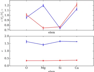
Figure 6.Upper panel: correction factors, the empirical yield to theoretical yield ratio,áYXemp,IIñ áYXtheo,IIñ, inferred to reproduce the observed [X/Fe]

values in the“thigh,”for theα-elements considered in this study and for both halo populations in the APOGEE sample. Bottom panel: efﬁciency of the SFR,

ν. The error bars show the values derived from the limits of theMuprange inferred of each population.

Figure 7. Parameters inferred from the “shin” (between [Fe H]knee and [Fe H]h). Top panel: fraction of SN Ia that explode per each simple stellar

populations of 1Me. Bottom panel: fraction of SN Ia relative to the fraction of

(7)

4. X( )tj ~X Hj ´H, where H=0.7392 (Asplund et al.2005).

Therefore,

= -n

-( ) ( ) ( ) ( )

M t M 0 e R t, 6

gas gas 1

whereRis the fraction of the mass ejected into the ISM by the dying stars.

Fromt=0 untiltk, a left-inﬁnite“thigh,”weﬁnd that n

= á ñ

-( )t Y ( R t) ( )

X k X 1 k, 7

and we obtain ν. The bottom panel of Figure 6 shows the ν values forα-elements and each population.

Focusing on the “shin,”we compute thfrom n

- = á ñ- -

-( )t ( )t Y ( R t)( t) ( )

X h X k Xk h 1 h k. 8

Finally, we calculate the SFR for each population: n

= -n

-( )_t _M ( )_e ( ) ( )

SFR 0 R t. 9

gas 1

We computeRusing stellar ejecta by Kobayashi et al.(2006)

and Karakas et al. (2009). Before theknee, only massive stars contribute to the ISM, andR=0.061. After theknee, massive and intermediate-mass stars die, andR=0.158. We derive the

SFR(t) assuming tk=1 Gyr and Mgas( )0 =1M. These choices are motivated to easily obtain the SFHs for other tk and Mgas( )0 values. Figure9 exhibits the resulting SFR(t)for

the HMg and LMg, in blue and red, respectively. We show the SFH for each population consideringν obtained from Fe, due to the familiar time–metallicity relation.

Table4presents the times when theﬁnal enrichment occurs for the analyzed elements for each population.

4. Results

4.1. Chemical Trends

The resulting trends for both populations are characterized by[X/Fe]decreasing with[Fe/H]. From the weighted[X/Fe] means, we identify thekneein the distribution at approximately −1.0 in the case of the LMg population and approximately −0.4 for the HMg population. Figure 4reveals that there is a gap in the weighted mean abundance ratios between the two populations. This separation is lower for[Si/Fe]and [Ca/Fe] than for [O/Fe] and [Mg/Fe]. The latter exhibits the largest difference.

It is important to notice that our sample of halo stars detected in APOGEE covers a metallicity range that is broader than those in previous works. The HMg population includes objects with[Fe H]> -0.4. Other halo studies had not taken account of stars at larger metallicities because of the difﬁculty of distinguishing them from disk stars without precise kinematical data. The accurate radial velocities measured in APOGEE allow us to distinguish these halo objects at[Fe H]> -0.4. The halo sample revealed at such high [Fe/H] shows a signiﬁcant decreasing trend of[X/Fe]with[Fe/H]. This trend was suggested by a handful of objects in NS97 at[Fe/H]∼ −0.4, but it is now well-established in this work.

This broad range in metallicity reveals the knee for both populations. This fact allows us to compare the level of[X/Fe] in stars from each population formed before and after the main contribution of SN Ia to the ISM. Consequently, we are able to well-establish whether the HMg population is in fact α-enhanced relative to the LMg population. Since the contribution by SN Ia of the α-elements Si and Ca is larger than that of Mg, we want to conﬁrm that the enhancement observed in the[X/Fe]versus[Fe/H]space is also detectable in[X/H]versus[Fe/H]. From the weighted means, we obtain the α-to-hydrogen ratios by subtracting the corresponding mean[Fe/H]. Figure10shows the[X/H]mean abundances as a function of[Fe/H]for each population in the“thigh.”We see that the HMg population reaches higher[X/H]values than the LMg population at[Fe/H]∼−1. In addition, the former has its knee shifted to a higher [Fe/H] and includes stars with higher [Fe/H] than the latter (which do not show stars at

>

-[Fe H] 0.6dex—see Table1). This implies that the HMg population is also metal-enriched relative to the LMg population.

As detected in previous works, we see that the separation between the two populations depends on the element considered. Besides, although all the APOGEE-reliableα-elements show a decrease of [X/Fe] with [Fe/H], the slope differs from one element to another, especially at the lowest metallicities. This is, however, expected since the yields from the very massive progenitor stars for these very metal-poor objects are different for each element. However, the slope of[Mg/Fe]with [Fe/H]

Figure 8.Percentage contribution by SN II(cyan)and SN Ia(magenta)to the

(8)

from the kneeup to[Fe H]h in the LMg is less steep than the slope at the same range in metallicity observed for[O/Fe]. This is not expected at all, considering the current yields of Mg and Fe for SN Ia, which predict a very low contribution of[Mg/H] and [O/H], and greater contributions of [Si/H] and [Ca/H]. Consequently, the slope would be similar to that for[O/Fe]and steeper than that observed for[Si/Fe]and[Ca/Fe]. This is not what we observed from our LMg chemical trends.[O/Fe],[Si/ Fe], and[Ca/Fe]exhibit similar slopes, which are steeper than for[Mg/Fe].

4.2. Inferences from the Chemical-evolution Models

As explained in Section 3.1, the star formation parameters are inferred by studying the two metallicity ranges: “thigh” and “shin.”

4.2.1. Upper Mass Limit for the IMF, Empirical Yields, and Star Formation Efﬁciency

We derived the Mup values for each halo population as described in Section3.1and Figure5. We obtain thatMupfor the HMg population (26.41.3M) is higher than for the LMg population (17.92.7M). Subsequently, the fraction

fSN IIderived for the HMg data is higher than that inferred from the LMg. The resulting values for both parameters are shown in Table 3. The fact that MupHMg>MupLMg implies that the HMg

population formed from an ISM polluted by more massive stars than the LMg population.

From the derived Mup values, and fixing the average Fe yields for massive stars, we obtain the correction factors for α-elements that should be applied to the theoretical yields tofit the abundance ratios. These are shown in the upper panel of Figure 6. We find that they are fairly well-approximated by unity. Thus, the derived Mup ranges are representative of the trueMupof each population.

In general, the correction factors for LMg are slightly higher than for the HMg, except for Mg. The difference between the Mg correction factors is the largest, due to the fact that the[Mg/H]difference between the HMg and the LMg is the highest among the fourα-elements (see Figure 10).

We also derive the star formation efﬁciency, ν, for each stellar population from each of the α-elements (see Equation (8)). The bottom panel in Figure 6 depicts the ν values. The efﬁciencies are in excellent agreement within the results from each elemental-abundance ratio. Besides, theνfor the HMg population is higher.

From Section 3.1, we infer the SFR as a function of time. Figure 9 shows the resulting SFR for both populations, as a function of time on the left, and as a function of[Fe/H]on the right. The equivalence between t and [Fe/H] is given by Equations(7)and (8).

The SFR for the HMg population is higher during most of the evolution and decreases more steeply than for the LMg population, becausenHMg>nLMg. The time at which the star

formation ends is lower for the LMg population, meaning a shorter SFH. In conclusion, our results imply that the HMg

Figure 9.SFR as a function of time(left panel)and[Fe/H](right panel). Vertical lines represent the time and[Fe/H]for thekneefor each stellar population. The

ﬁgure is color coded as in Figure4.

(9)

stars formed from a more efﬁcient and longer SFH than the LMg population.

4.2.2. Contribution of SN Ia and SN II in the“Shin”

It is well known that the steeper downward slope of[X/Fe] versus[Fe/H]beyond thekneeis due to the contribution of SN Ia. Therefore, we derive their contribution, taking into account the SN Ia yields and the empirical yields for SN II, the latter

Z-averaged at the metallicities in the“shin.”

The upper panel of Figure7shows the fraction of SN Ia that occurs in1Mof stellar mass. The resulting values,~10-3M, are on the order of thefSN Iaobserved in dwarf galaxies(Maoz et al. 2014). The results obtained from the four α-elements show different trends between the populations. However, our results suggest that there is not a signiﬁcant difference between the fraction of SN Ia that contributes to each population. The differences between populations are within the typical errors found in dwarf galaxies. The lowfSN Iavalue obtained from Mg is due to theﬂatter slope in the“shin”for the LMg population. The resultingfSN Iafrom O shows a larger value for the LMg population because the slope of its“shin”is steeper than for the HMg population.

Figure 8 exhibits the percentage contribution of SN II and SN Ia to the α-element enrichment during the “shin.” As expected, in this metallicity range, the main contribution to O

and Mg is due to SN II, whereas Si and Ca have important contributions(~35%and~15%, respectively)from SN Ia.

5. Discussion

We have explored and modeled the chemical evolution of the two halo populations seen clearly in APOGEE data, as described in Paper I.

Halo stars selected by their large radial velocities and a non-disk-like motion in the GRV/cos(b)versuslspace within the

APOGEE DR13 database cover a metallicity range

−2.2<[Fe/H]<+0.5. This broad range in metallicity reveals the kneefor the two halo populations. The metal-rich side of the HMg population was unexplored in previous works (Nissen & Schuster papers; Hawkins et al.2015; Paper I). The population with higher α-to-iron ratios was truncated at−0.4 or lower metallicities in their samples, and the high-[α/Fe] trend with metallicity was described as ﬂat and constant. Our work reveals that this population also shows a steeper decreasing trend at higher metallicities, similar to the decrease observed in the NS10low-αpopulation, which they ascribed to an increase of iron abundance in the ISM from the contribution of Type Ia supernovae.

NS10 and later works tried to explain the chemical differences observed between populations in the metallicity range−1.6<[Fe/H]<−0.4 in terms of the contribution of SN Ia for thelow-αpopulation due to a lower SFH. The SFH of the high-α population should have been faster in order to reach larger metallicities without the contribution of SN Ia. Kobayashi et al. (2014) pointed out that these chemical differences observed between populations could be accounted for by yields from massive stars between 10 and 20 solar masses. They suggested that there could be a difference in the IMF that led to the differences detected in the chemical abundances.

Table 3

Upper Mass Limit for the IMF Determined from the Observed[X/Fe](see Figure5), and the SubsequentfSN II

Population Mup(M) fSN II(10−

3 )

HMg 26.4±1.3 4.59±0.1

LMg 17.9±2.7 4.00±0.4

Table 1

Halo Stars Selected within the DR13 APOGEE Database, with the Stellar Atmospheric Parameters and Chemical Abundances Determined by ASPCAP and Used in This Worka

2MASS ID Population Teff logg vrad [Fe H] [O Fe] [Mg Fe] [Si Fe] [Ca Fe]

2M13590274+0118564 HMg 4486 1.0 259.790 −1.95 0.53 0.39 0.27 0.29

2M23161405+1257322 HMg 4435 1.1 −179.804 −1.86 0.30 0.49 0.66 0.16

2M10374221−1042328 HMg 4346 1.2 181.805 −1.34 0.43 0.31 0.12 0.43

2M11002833−1044050 HMg 4483 1.1 337.768 −1.28 L 0.31 0.40 0.38

2M11422622−1409451 HMg 4323 1.2 258.096 −1.20 0.36 0.24 0.20 0.33

Note.

a

Full table is available at the CDS.

(This table is available in its entirety in machine-readable form.)

Table 2

Mean[Fe/H]and[X/Fe]Derived from the Two Stellar Populations at the Key[Fe/H]values

Population Element [Fe H]l [X Fe]l [Fe H]k [X Fe]k [Fe H]h [X Fe]h

HMg O −1.46±0.15 0.37±0.03 −0.43±0.02 0.20±0.01 0.08±0.09 0.09±0.01 Mg −1.48±0.13 0.34±0.04 −0.43±0.02 0.26±0.01 0.09±0.08 0.09±0.03 Si −1.56±0.14 0.30±0.05 −0.43±0.02 0.16±0.03 0.08±0.08 0.02±0.02 Ca −1.51±0.14 0.36±0.09 −0.44±0.02 0.14±0.01 0.09±0.07 0.03±0.01

(10)

However, it is important to notice that they were trying to explain chemical differences in objects that would have formed from an ISM enriched before and after the pollution by SN Ia (the high-α and low-α population, respectively). Since we detect the metallicity value at which the contribution of SN Ia became relevant, we are able to compare those objects from each stellar population, which had the same kind of progenitors. Therefore, we are able to clarify their hypothesis. On the one hand, we see that the metallicity range analyzed by Nissen & Schuster (−1.6<[Fe/H]<−0.4) comprises objects before thekneefor the HMg population and before and after thekneefor the LMg population. This fact implies that the differences observed are, at least partially, due to the contribution of SN Ia, as NS10 suggested. On the other hand, the inference of the IMF upper mass limit from objects before thekneefor both populations lets us ascertain whether there is, in addition, a difference in the IMF between the populations. We obtain that there is actually a difference in the IMF. Besides, we derive that the upper mass limit for the LMg population is between 10 and 20 solar masses, as pointed by Kobayashi et al. (2014). Therefore, we conclude that the chemical differences previously detected by NS are due to the combination of a difference in the IMF as well as the con-tribution of SN Ia for the LMg stars at metallicities lower than −0.4, at which point there was not yet a contribution of SN Ia for the HMg population.

The parameters inferred from these two different chemical trends lead us to two populations with different SFHs:

1. one population with an IMF weighted to more massive stars, and an SFR more intense and extended in time, and 2. a second population with a top-lighter IMF, and a lower

and shorter SFH.

The SFR(t)from the HMg stars behaves similarly to that of the inner Galactic disk (r~4 kpc) during the last 10 Gyr, while the SFR(t) from the LMg stars resembles that of the intermediate Galactic disk (r~8 kpc) during the last 7 Gyr (Carigi & Peimbert2008). Both regions of the Milky Way disk are explained assuming an inside-out scenario (see Carigi & Peimbert2008,2011). Therefore, we also may explain the two halo populations as resulting from an inside-out scenario for halo formation, where ﬁrst the HMg stars formed in the inner halo, and immediately after the LMg stars formed in the outer halo. The IMF for the inner halo needs to be top-heavier to match its α-enhancement, and the outer halo requires a

dynamically disrupted component to reproduce the retrograde mean orbit observed by NS10.

On the other hand, our results are also consistent with massive satellites reaching and populating more inner regions within the host galaxy during its formation(Tissera et al.2014; Amorisco 2017). The more massive the satellites are able to continue star formation after they enter the virial radius of the host galaxy. This implies that their SFR would be more extended in time. The less massive satellites would not be able to survive inside the galactic potential, which means that they would be likely to populate the outer regions. They will be disrupted and their star formation would cease. Their SFR before the disruption would be lower because of their lower masses.

Recent results have shown that the top-mass end of the IMF may vary from galaxy to galaxy and across the galaxies to explain the dark-matter and baryonic mass-to-light ratio (Cappellari et al. 2012; Lyubenova et al. 2016). Even more, variations are also found across each galaxy, with clear correlations with the stellar metallicity (Martín-Navarro et al.

2015). An IMF dominated at early times by high-mass stars would also produce an enhanced [Mg/Fe] (Martín-Navarro et al. 2015), presenting old stellar populations and being produced by a strong and short star formation event(Walcher et al.2015). This agrees with our results indicating that HMg stars were formed in a stronger star formation event, with a shorter decline time than LHg ones.

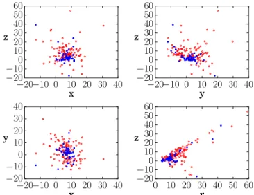
Figure11shows the space distribution of our sample, using distances from the BPG(Santiago et al.2016). From thexy,yz, and xz planes(in Galactic coordinates), we see that the HMg population is mainly conﬁned at inner regions of the halo. The bottom right panel shows the distance from the Galactic plane,

z, as a function of distance from the Galactic center, r. The HMg stars are concentrated nearer the Galactic plane (∣ ∣z  5 kpc) and the LMg stars reach to larger distances from the center of the Galaxy(r15kpc)and from the Galactic plane. This is consistent with our previous conclusions.

(11)

The abundance dispersion is larger for the LMg population than for the HMg population. It is also larger than the errors in the measurements. This fact suggests that this LMg sample is comprised of several populations, i.e., stars formed from environments with different previous enrichments. Moreover, the dispersion may also be caused by the stochastic pollution by massive stars, as the stochastic effects are more relevant when massive stars die in a metal-poor ISM inside small satellites (Carigi & Hernandez2008).

We assume a simple chemical-evolution model that is able to reproduce the chemical trends observed. We do not need to claim for inﬂows or outﬂows. However, a kinematical analysis with the precise data provided in the following Gaia data releases will help to reveal the origin of the stars and better clarify the stellar populations comprised in our sample and their chemical trends. A more complex chemical-evolution model might be necessary then. It is also necessary to establish with simulations the accretion history of the Galaxy, and better establish whether the chemical trends observed in halo stars could be the result of an inside-out scenario or different kinds of satellites accreted at different times from the host halo of the Galaxy.

6. Summary and Conclusions

We evaluate chemical trends in the[X/Fe]versus[Fe/H]space from 175 stars selected within the DR13 APOGEE database, at

<T <

4000 eff 4500K, for which abundances of theα-elements

O, Mg, Si, and Ca calculated by ASPCAP have the highest accuracy(mean uncertainties∼0.05 dex). We infer the IMF upper mass limit, fractions of SN II and SN Ia relative to the total stellar population, and the star formation efﬁciency, following a closed-box model of the chemical evolution of the Galaxy under a semi-instantaneous recycling approximation.

We obtain the following:

1. Two populations are distinguishable for eachα-element in the [X/Fe]versus [Fe/H]space. Their[α/Fe]versus [Fe/H]trends are in agreement with those found by NS10 and NS11 for halo stars.

2. The metallicity range covered extends, at both the low-and high-metallicity limits, beyond that analyzed for the two halo populations previously. This is theﬁrst time that these two populations are analyzed over the range-2.2<

< +

[Fe H] 0.5.

3. Both populations exhibit a decreasing α-to-iron abun-dance trend associated with Fe enrichment of the ISM by SN Ia. This change in the slope(at−0.4 and−1.0 for the HMg and LMg populations, respectively) is also observed for all the α-elements examined, except Ti. 4. Thus, we compare stars before thekneeand beyond the

knee, i.e., objects formed from an ISM with the contribution of only SN II and objects from an ISM with the additional contribution of SN Ia. This permits a proper comparison between both populations, in order to clarify whether one population is α-enhanced with respect to the other. We corroborate that the population with higherα-to-iron values revealed by NS10 is in fact α-enhanced with respect to the other. Besides, this population is also metal-enriched with respect to the LMg population.

5. According to our closed-box model, more massive stars contribute to the ISM where the HMg formed with

respect to the LMg population, which implies an IMF weighted to a higher upper mass limit.

6. There is no signiﬁcant difference between the two populations regarding the contribution of SN Ia to enrich the ISM from which the populations formed.

7. The SFR was higher in the HMg population, decreases more steeply with time, and was longer than the SFR(t)

inferred for the LMg population. The latter was lower at early times, more constant, and shorter.

E.F.A. acknowledges support from DGAPA-UNAM post-doctoral fellowships. L.C. is thankful for thefinancial support provided by CONACyT of México(grant 241732), by PAPIIT of México (IG100115, IA101215, IA101517), and by MINECO of Spain (AYA2015-65205-P). W.J.S. is thankful for the financial support provided by PAPIIT of México (IN103014). C.R.H. and S.R.M. acknowledge NSF grants AST-1312863 and AST-1616636. C.A.P. is thankful to the Spanish Government for funding for his research through grant AYA-2014-56359-P. T.C.B. acknowledges partial support from grant PHY 14-30152; Physics Frontier Center/JINA Center for the Evolution of the Elements(JINA-CEE), awarded by the US National Science Foundation. D.A.G.H. was funded by the Ramn y Cajal fellowship number RYC-2013-14182. D.A.G.H. and O.Z. acknowledge support provided by the Spanish Ministry of Economy and Competitiveness(MINECO) under grant AYA-2014-58082-P. B.T., J.F.-T., and D.G. gratefully acknowledge support from the Chilean BASAL Centro de Excelencia en Astrofísica y Tecnologías Afines (CATA)grant PFB-06/2007. S.V. gratefully acknowledges the support provided by Fondecyt reg. 1170518.

(12)

Cosmic Abundances as Records of Stellar Evolution and Nucleosynthesis, ed. F. N. Bash & T. G. Barnes(San Francisco: ASP),25

Avila-Vergara, N., Carigi, L., Hidalgo, S. L., & Durazo, R. 2016,MNRAS,

457, 4012

Beers, T. C., Carollo, D., Ivezic, Z., et al. 2012,ApJ,746, 34

Belokurov, V., Irwin, M. J., Koposov, S. E., et al. 2014,MNRAS,441, 2124

Bernard, E. J., Ferguson, A. M. N., Schlaﬂy, E. F., et al. 2016, MNRAS,

463, 1759

Bertran de Lis, S., Allende Prieto, C., Majewski, S. R., et al. 2016,A&A,590, A74

Blanton, M. R., Bershady, M. A., Abolfathi, B., et al. 2017,AJ,154, 28

Brunthaler, A., Reid, M. J., Menten, K. M., et al. 2011,AN,332, 461

Cappellari, M., McDermid, R. M., Alatalo, K., et al. 2012,Natur,484, 485

Carigi, L., & Hernandez, X. 2008,MNRAS,390, 582

Carigi, L., & Peimbert, M. 2008, RMxAA,44, 341

Carigi, L., & Peimbert, M. 2011, RMxAA,47, 139

Carlberg, R. G., Grillmair, C. J., & Hetherington, N. 2012,ApJ,760, 75

Carlin, J. L., Liu, C., Newberg, H.-J., et al. 2016,ApJ,822, 16

Carollo, D., Beers, T. C., Chiba, M., et al. 2010,ApJ,712, 692

Carollo, D., Beers, T. C., Lee, Y. S., et al. 2007,Natur,450, 1020

Chiba, M., & Beers, T. C. 2000,AJ,119, 2843

de Jong, J. T. A., Yanny, B., Rix, H.-W., et al. 2010,ApJ,714, 663

De Lucia, G. 2012,AN,333, 460

Duffau, S., Vivas, A. K., Zinn, R., Méndez, R. A., & Ruiz, M. T. 2014,A&A,

566, A118

Eggen, O. J., Lynden-Bell, D., & Sandage, A. R. 1962,ApJ,136, 748(ELS) Eisenstein, D. J., Weinberg, D. H., Agol, E., et al. 2011,AJ,142, 72

Fernández-Alvar, E., Allende Prieto, C., Schlesinger, K. J., et al. 2015,A&A,

577, 81

Franco, I., & Carigi, L. 2008, RMxAA,44, 311

Fulbright, J. P. 2002,AJ,123, 404

García Pérez, A. E., Allende Prieto, C., Holtzman, J. A., et al. 2016,AJ,151, 144

Gilmore, G., Wyse, R. F. G., & Kuijken, K. 1989,ARA&A,27, 555

Gratton, R. G., Carretta, E., Desidera, S., et al. 2003,A&A,406, 131

Gunn, J. E., Siegmund, W. A., Mannery, E. J., et al. 2006,AJ,131, 2332

Hawkins, K., Jofré, P., Masseron, T., & Gilmore, G. 2015,MNRAS,453, 758

Hayden, M. R., Bovy, J., Holtzman, J. A., et al. 2015,ApJ,808, 132

Hayes, C. R., Majewski, S. R., Shetrone, M., et al. 2017, in press(arXiv:1711. 05781)

Helmi, A. 2008,A&ARv,15, 145

Hernández-Martínez, L., Carigi, L., Peña, M., & Peimbert, M. 2011, A&A,

535, 118

Marín-Franch, A., Aparicio, A., Piotto, G., et al. 2009,ApJ,694, 1498

Márquez, A., & Schuster, W. J. 1994, A&AS,108, 341

Martín-Navarro, I., Vazdekis, A., La Barbera, F., et al. 2015,ApJL,806, L31

Mészáros, S., Martell, S. L., Shetrone, M., et al. 2015,AJ,149, 153

Mihalas, D., & Binney, J. 1981, Galactic Astronomy: Structure and Kinematics (San Francisco, CA: Freeman)

Morrison, H. L., Helmi, A., Sun, J., et al. 2009,ApJ,694, 130

Nidever, D. L., Holtzman, J. A., Allende Prieto, C., et al. 2015,AJ,150, 173

Nissen, P. E., & Schuster, W. J. 1997, A&A,326, 751

Nissen, P. E., & Schuster, W. J. 2010,A&A,511, L10(NS10) Nissen, P. E., & Schuster, W. J. 2011,A&A,530, A15(NS11) Norris, J. E., Bessell, M. S., & Pickles, A. J. 1985,ApJS,58, 463

Ramírez, I., Meléndez, J., & Chaname, J. 2012,ApJ,757, 164

Robles-Valdez, F., Carigi, L., & Peimbert, M. 2013,MNRAS,429, 235

Romano, D., Karakas, A. I., Tosi, M., & Matteucci, F. 2010,A&A,522, A32

Sandage, A. 1986,ARA&A,24, 421

Santiago, B. X., Brauer, D. E., Anders, F., et al. 2016,A&A,585, A42

Schlaufman, K. C., Rockosi, C. M., Allende Prieto, C., et al. 2009,ApJ,

703, 2177

Schlaufman, K. C., Rockosi, C. M., Lee, Y. S., et al. 2012,ApJ,749, 77

Schlaufman, K. C., Rockosi, C. M., Lee, Y. S., Beers, T. C., & Allende Prieto, C. 2011,ApJ,734, 49

Schönrich, R. 2012,MNRAS,427, 274

Schuster, W. J., Moreno, E., Nissen, P. E., & Pichardo, B. 2012,A&A,538, A21

Searle, L., & Zinn, R. 1978,ApJ,225, 357(SZ)