Beyond the quasistatic approximation: Impedance and capacitance of an exponential distribution of traps

Texto completo

(1)PHYSICAL REVIEW B 77, 235203 共2008兲. Beyond the quasistatic approximation: Impedance and capacitance of an exponential distribution of traps Juan Bisquert* Departament de Física, Universitat Jaume I, 12071 Castelló, Spain 共Received 9 November 2007; revised manuscript received 1 March 2008; published 9 June 2008兲 Electronic carriers in disordered organic and inorganic semiconductor materials, used in electronic, optoelectronic, and photovoltaic devices, are usually affected by an exponential distribution of localized states in the band gap 共traps兲. In this paper we provide a full solution of the relaxation of carriers in traps of such distribution, as a function of frequency and steady-state Fermi level. This includes in a unified treatment both the quasistatic limit, in which the traps modify time constants such as the trap-limited mobility, and the power-law relaxation at high frequency due to detrapping kinetics. We also analyze the combination of trapping with diffusion transport and recombination dynamics in photovoltaic devices. The different features of impedance and capacitance spectra are interpreted and also the analysis of the spectra in order to derive the main material parameters. DOI: 10.1103/PhysRevB.77.235203. PACS number共s兲: 73.23.⫺b, 72.20.Jv, 73.61.Ph. I. INTRODUCTION. Disordered organic and inorganic materials have raised increasing attention in the last two decades, in relation with applications in devices such as dye-sensitized solar cells 共DSCs兲,1,2 plastic solar cells,3,4 organic light-emitting diodes 共OLEDs兲,5 and organic electronics.6 Frequency domain techniques are becoming of widespread used in the study of these materials and devices, since they provide an insight both on fundamental electronic processes and global device properties. Impedance and capacitance spectroscopy of devices7,8 using such materials normally requires to consider a distribution of states in energy. Energy disorder is common for band-gap states of electronic carriers in disordered semiconductors, both for nanostructured metal oxides used in DSC 共Refs. 9 and 10兲 and for organic conductors used in thin-film transistors 共TFT兲,11–13 OLEDs,8,14 and organic solar cells.15 Especially in organic materials, deep traps are reactive sites as they are either radical cations or anions and can play a role in the degradation of organic molecules, such as polyphenylvinylene polymers. However, the degradation occurs at time scales of thousands of hours in the most stable systems. An important factor is therefore the presence of impurities which can also act as trapping sites, extrinsic traps, which can greatly influence the stability of the system. Also in ionic materials such as Li battery cathodes, energetic inhomogeneity has been found.16 The exponential distribution of states seems to play a key role in many of the mentioned systems. For example, such distribution is routinely obtained as a chemical capacitance in electrochemical measurements of nanostructured TiO2 共Refs. 17 and 18兲 and the exponential density of states 共DOS兲 also explains the observed variation of electron diffusion coefficient in DSC using multiple trapping arguments.9,10 The exponential DOS is also often employed in connection with organic conductor materials.8,12–15 Closely connected to such a distribution is the anomalous diffusion model19 that so far seems to be the best approach for interpretation of diffusion of guest ions in transitionmetal oxides.20,21 1098-0121/2008/77共23兲/235203共15兲. Most of the work presented in the literature for the interpretations of these systems uses a multiple trapping model, where the effect of traps is to reduce the mobility and increase the recombination time by a factor of the free to trapped charge. This approach, which dates back to Rose,22,23 is formulated as a quasistatic approximation in Refs. 24 and 25 and has been widely used in the DSC area.10,26 Similar approaches to trap-limited mobility are well known in the field of crystalline organic electronic devices27 and amorphous organic semiconductors.8,11 This approximation is quite useful since it allows us to treat the trap distribution simply as an additional charge, which follows the relaxation of the free charge in the system, so that the time constants in the system can be easily deduced using the kinetic model of the trap-free system. However, any relaxation of the trapped carriers is assumed to be very fast and is neglected from the beginning. However, if the trap distribution indeed exists, one should be able to observe the relaxation of trappingdetrapping kinetics, provided that one measures in the appropriate frequency domain. A direct measurement of trap kinetics is very important for tailoring the materials with required properties for device operation. There exist classical results on dispersive 共power-law兲 behavior of the photoconductivity and mobility in time transient experiments, which is due completely to the trapping kinetics.28,29 Therefore, one can switch from the regime, where the traps remain in equilibrium, to that in which they dominate the transient response.30 In this paper we provide a full solution of the relaxation of the exponential distribution of traps, which unifies both regimes of behavior in a single framework, in the frequency domain. It is well known that in semiconductor devices, each trap level provides a series RC circuit.31 The capacitance Ctrap is the chemical capacitance of a localized state32 and relates to the equilibrium occupancy of the trap f̄ 共with 0 ⱕ f ⱕ 1兲 as Ctrap ⬀ f̄共1 − f̄兲. It should be emphasized that Ctrap is related to the variation of the occupation of the trap with respect to the quasi-Fermi level. So this capacitance has nothing to do with a standard dielectric capacitance and is more related to the chemical capacitance,17,33 also known as accumulation. 235203-1. ©2008 The American Physical Society.

(2) PHYSICAL REVIEW B 77, 235203 共2008兲. JUAN BISQUERT. Extended states Potential. “shallow” states. Fermi level. “deep” states Localized states. FIG. 1. 共Color online兲 The scheme shows a semiconductor where the Fermi level can be controlled with external potential. The semiconductor has both extended states 共e.g., conduction-band levels兲 and localized 共band-gap兲 levels. The Fermi-level marks approximately the separation between occupied and empty localized levels, which applies in an exponential distribution of traps. The equivalent circuit for two specific levels 共one occupied, another one empty兲 is shown. For each level, the resistance corresponds to the thermal release of electron to the extended levels, and the capacitance corresponds to the variation of equilibrium occupancy of the level under variation of Fermi level, i.e., a chemical capacitance. The extended states also possess a chemical capacitance, though this is not shown. The characteristic frequencies of the equivalent circuits of occupied and empty levels have different properties, as discussed in the text, and are denoted as “deep” and “shallow,” respectively.. capacitance34 or redox capacitance.35 On another hand the resistance Rtrap contains the kinetic factor for detrapping. Both values depend on the occupancy of the level, and the characteristic trap frequency is given by. ␻t =. 1 . RtrapCtrap. 共1兲. The value of ␻t determines the relaxation properties of each level in the distribution. The properties of simple trap combinations in the frequency domain are illustrated in Appendix. We have discussed in detail in a previous paper the frequency-dependent capacitance in a two-state model,36 and this model has been successfully applied in experiments of ion insertion in metal oxides.16 Using a similar method we provide here a full solution of the capacitance and impedance of the exponential DOS. Since the characteristic time for detrapping depends exponentially on the distance between a trap level and the transport level, the exponential distribution introduces a very large set of time scales. Furthermore, the trap response is largely variable depending on the occupancy of the trap. Therefore, it is required to establish the steady state of the DOS, at given Fermi level, as indicated in Fig. 1, and then to calculate the frequency-dependent capacitance Cⴱ共␻兲, by integration of the capacitance of the different levels, and the associated impedance, Z共␻兲 = 1 / i␻Cⴱ共␻兲. By summation, we give here a closed expression for the capacitance Cⴱ共␻兲 of the whole distribution in a good approximation. Very often, in experimental spectra, several frequency effects due to distinct phenomena 共e.g., energy disorder and. geometry inhomogeneity16兲 have to be deconvoluted. For the interpretation of experimental data, it is very useful to have an understanding, in terms of analytical models, of the different spectral features in separate segments of the frequency window of measurement. Therefore, we will develop analytic approximations to the whole response of the exponential distribution of traps. The shape of spectra and different behaviors obtained at low and high frequencies will be discussed in detail, as well as the dependence of parameters on steady-state conditions, in order to assist the interpretation of experimental data. The paper is divided into two main parts. Section II treats the relaxation of a continuous distribution of traps in the frequency domain, as shown schematically in Fig. 1. The goal of this section is to find out the local effects caused by the trapping-detrapping phenomena when all the states of the distribution are considered simultaneously. Section III describes an approach to spatially extended device modeling, by considering diffusion trapping in a restricted layer, and the effect of the trap distribution on recombination dynamics in the frequency domain, mainly in relation with photovoltaic systems such as DSC. We expect that these results will find application in a wider variety of systems. In this work we restrict our attention to systems in which the Fermi level can be considered homogeneous across the active device layer. We plan to apply the present developments in highly inhomogeneous systems such as TFTs and OLEDs in a future work. Another interesting development left for the future is to apply a similar method to the Gaussian distribution that is also widely used in organic semiconductors.25,37 II. TRAP MODEL. Figure 1 shows a basic scheme of the model discussed in this paper. The scheme shows a piece of semiconductor, both with a transport level 共extended states兲, and localized states in the band gap. The traps are assumed to be connected 共by trapping-detrapping kinetics兲 to the transport level, which communicates with the outer contacts. In the scheme, we indicate that the applied potential governs the Fermi level 共a specific realization of this is shown in Fig. 8; see also Ref. 2兲. Therefore, we assume that the local Fermi level can be fixed at a value EF. The measurement involves two levels of perturbation. The first is the steady-state value of the potential. This fixes the occupation of the traps and the free-carrier concentration. More generally, if the traps also serve as recombination centers, they are normally not in thermal equilibrium with the conduction-band carriers, and they require separate Fermi levels.38,39 However, in the present work we do not treat such situation, and the traps are conservative with respect to number of carriers. The second level is a small harmonic perturbation. The latter causes the dynamic response of the traps and facilitates the analysis of experimental systems by looking at the spectral features of the capacitance and impedance. In essence the frequency response of a trap is a RC series circuit, as shown in Fig. 1 for two traps and discussed in Appendix. However, there is a great difference of trap response according to their steady-state occupancy. The empty. 235203-2.

(3) PHYSICAL REVIEW B 77, 235203 共2008兲. BEYOND THE QUASISTATIC APPROXIMATION:…. ⳵ ft = ␤nc关1 − f t兴 − ␧f t . ⳵t. 共5兲. Here, ␤ is the time constant for electron capture, usually given in terms of the thermal velocity of the electrons and capture cross section,. ␤ = v␴n . 共5兲. In steady state, at given Fermi level EF, we have from Eq.. f̄ t = FIG. 2. 共Color online兲共a兲 Energy diagram showing the thermal occupation at temperature T = 300 K of an exponential DOS in the band gap. EF is the Fermi level of electrons and Ec is the conduction-band energy. The clear 共green兲 shaded region indicates the band-gap states that are occupied with electrons, and the dark 共blue兲 shaded region indicates empty levels, as determined by the Fermi–Dirac distribution function 共red dashed line兲. 共b兲 The trap frequencies as a function of energy. The parameters used in the calculation: T0 = 800 K, Nc = 1020 cm−3, Nt = 1020 cm−3, and ␤ = 10−10 cm2 s−1.. traps readily capture electrons, while the full traps do not. More exactly, the occupation of electron traps above the Fermi is well approximated by the Boltzmann distribution. Below the Fermi level, traps are almost fully occupied, but the density of vacant traps 共holes兲 also obeys the Boltzmann distribution. The occupations are quantitatively shown in Fig. 2共a兲 in the energy axis. The aim of the following development is to obtain the characteristic spectra of the combined relaxation of all the traps in the exponential distribution. A. Kinetic equations. The model is formulated assuming the extended states at the level Ec 共conduction-band edge兲, with effective density Nc and number density of carriers nc. With respect to the Fermi level EF, we have nc = Nce共EF−Ec兲/kBT ,. nt =. 冕. Ec. g共E兲f t共E兲dE.. 共3兲. 1 1 + ␧/共␤n̄c兲. F共E,EF兲 =. ⳵ nc ⳵ nt =− =− ⳵t ⳵t. 冕. Ec. Ev. ⳵ ft g共E兲 dE, ⳵t. 共4兲. 共7兲. 1 . 1 + e共E−EF兲/kBT. 共8兲. By detailed balance condition, the time constant for release from the traps at the energy Et is ␧共Et兲 = ␤Nce共Et−Ec兲/kBT .. 共9兲. B. Frequency-dependent capacitance of a trap distribution. The method to obtain the frequency-dependent capacitance is explained in detail in Ref. 36. Let us denote steadystate quantities by ȳ and small perturbation quantities by ŷ. The capacitance is the relation of ac charge 共Q̂兲 to voltage 共V̂兲, C ⴱ共 ␻ 兲 =. Q̂ V̂. =. q V̂. 共n̂c + n̂t兲 =. q V̂. 冉冕. Ec. n̂c +. Ev. 冊. g共E兲f̂ tdE , 共10兲. where q is the positive elementary charge. Note that all capacitances C in this section are given per unit volume. The extended states follow instantaneously the variation of applied voltage, which causes a variation of the Fermi level of the free electrons in the conduction band, −qdV = dEF. 共This assumption involves infinitely fast transport in the extended states and will be relaxed in Sec. III.兲 Therefore, we can use the relationship n̂c =. dn̄c. V̂.. dV̄. 共11兲. This last equation can be expressed n̂c =. C0 V̂ q. 共12兲. in terms of the chemical capacitance of the extended states,17,33. Ev. For the sake of brevity we omit the argument of f t in the following. The kinetic equations are. = F共Et,EF兲. in terms of the Fermi–Dirac function,. 共2兲. where kB is Boltzmann’s constant and T the temperature. In addition, we assume a distribution of traps g共E兲, with occupancy f t共E兲, where E is the energy; see the diagram in Fig. 2共a兲 that illustrates the exponential distribution. The number of density of carriers in trap states is. 共6兲. C0 = q. dn̄c dV̄. =. q2 n̄c . k BT. 共13兲. In contrast to Eq. 共11兲, the traps do not follow instantaneously the voltage variation, since each trap only communicates with the conduction band. By solving Eq. 共5兲 for a small perturbation, we obtain. 235203-3.

(4) PHYSICAL REVIEW B 77, 235203 共2008兲. JUAN BISQUERT. (a) C0. rt0. rt1. rtm. ct0. ct1. ctm. conduction band. n̂t =. traps. (c). (b). C0. C0. “shallow” levels. Qa. Ztraps FIG. 3. 共a兲 The equivalent circuit of the conduction-band states 共represented by capacitance C0兲 and the distribution of traps, each energy interval dE being associated with a RC circuit. 共b兲 The trap impedance is represented by Ztraps. 共c兲 Reduction of the impedance of an exponential distribution of traps Ztraps to a much simpler equivalent circuit, valid in the high-frequency domain, as is demonstrated quantitatively in the text. The sum of individual RC elements, each corresponding to a narrow energy interval, over all the shallow levels 共above the Fermi level兲 collapses into a CPE element.. f̂ t =. 1 f̄ t共1 − f̄ t兲 n̄c 1 + i␻/␻t. n̂c ,. 共14兲. where the trap frequency has the expression. ␻t =. ␧. .. 1 − f̄ t. 共15兲. From Eqs. 共12兲 and 共14兲 we obtain that the trap occupancy depends on the frequency as f̂ t =. q f̄ t共1 − f̄ t兲 V̂. k BT 1 + i ␻ / ␻ t. 共16兲. C. Characteristic trap frequencies. Let us discuss the dependence of characteristic frequencies 关Eq. 共15兲兴 on the trap energies using approximations to the Fermi–Dirac distribution f̄ t. For Et ⬍ EF, the trap frequency is constant,. ␻t0 = ␤n̄c ⬇ ␤Nce−共Ec−EF兲/kBT . 共17兲. The second term in Eq. 共17兲 is the frequency-dependent capacitance of the trap distribution. It has the form ⴱ 共␻兲 = Ctraps. 冕. Ec. Ev. Ct共E兲 dE, 1 + i␻/␻t. 共18兲. where Ct共E兲 is the equilibrium chemical capacitance per unit energy,32. ␻t共Et兲 ⬇ ␤Nce−共Ec−Et兲/kBT .. 共22兲. These results are illustrated in Fig. 2共b兲 and are independent of the distribution g共E兲, provided that the approximation of the Boltzmann distribution can be used, as already mentioned. The different dependence of ␻t below and above EF makes it a useful step to split the integral in Eq. 共18兲 in two parts, ⴱ ⴱ ⴱ Ctraps 共␻兲 = Ctraps 共␻兲 + Ctraps 共␻兲 ⬅. 共19兲. so that CtdE is the capacitance associated to the traps in the interval dE. Equation 共18兲 means a parallel connection of all the separate capacitances of the traps, as indicated in Fig. 3. Integrating Eq. 共14兲 over the energy axis, we can write the relationship between ac modulation of trapped and free carriers as. 共21兲. On another hand, for Et ⬎ EF the trap frequency increases with Et,. 2. q Ct共E兲 = g共E兲f̄ t共1 − f̄ t兲, k BT. 共20兲. From Eqs. 共18兲 and 共19兲 a numerical calculation of the frequency-dependent trap capacitance, at given Fermi level, is now possible and will be used below to plot the exact results. As indicated above, we also wish to understand the separate features of the spectra in different ranges of the frequency domain. According to Eq. 共9兲 the levels below EF are almost fully occupied, while the levels above EF are populated following the Boltzmann distribution: f t = e−共E−EF兲/kBT 关see Fig. 2共a兲兴. This makes a great difference for the kinetics of the traps; therefore, a main distinction in the calculation below is made for trap levels above and below the Fermi level. We have denoted them, respectively, as “shallow” and “deep” traps, as indicated in Fig. 1. This is a convenient notation for the purpose of the model that does not imply that either kind of trap is close or far from the transport level in an absolute sense. In addition, the Boltzmann statistics can also be used to describe vacant states below the Fermi level. The use of the Boltzmann statistics, to describe the trap occupancy in suitable domains of the energy axis, is a good approximation for the exponential distribution and other distributions. However, in other cases, such as the Gaussian distribution when the Fermi level is deep, this approach fails. Indeed the carrier occupation at low carrier density has the form of a Gaussian distribution around ␴2d / kBT below the center of the DOS 共Ref. 37兲共see Ref. 25 for a discussion of this question兲. Thus, the Gaussian distribution requires a separate treatment.. Inserting Eqs. 共13兲 and 共16兲 in Eq. 共10兲, we obtain ⴱ 共␻兲. Cⴱ共␻兲 = C0 + Ctraps. ⴱ 共␻兲 Ctraps n̂c . C0. +. 冕. 冕. EF. Ev. Ec. EF. Ct共E兲 dE 1 + i␻/␻t. Ct共E兲 dE. 1 + i␻/␻t. 共23兲. D. Capacitance of deep levels. According to Eq. 共21兲, all the occupied sites bellow EF 共which we will call the deep levels兲 relax with the same. 235203-4.

(5) PHYSICAL REVIEW B 77, 235203 共2008兲. BEYOND THE QUASISTATIC APPROXIMATION:…. frequency, ␻t0, which is also the slowest frequency in the distribution. We can immediately infer that the deep levels can be described as a RC series circuit, ⴱ 共␻兲 = Cdeep. Cdeep0 . 1 + i␻/␻t. 冕. q2 k BT. EF. g共E兲f̄ t共1 − f̄ t兲dE.. 1 . ␻t0Cdeep0. Ctraps =. q k BT. Rdeep =. 冕. Ec. g共E兲f̄ t共1 − f̄ t兲dE.. 共27兲. Ev. In this case, the traps and extended state occupation remain in equilibrium throughout the measurement, so there are no kinetic manifestations of the traps. This forms the basis for the quasistatic approximation to multiple trapping systems, which will be shown in detail in Sec. III, below. With respect to the shallow levels, at Et ⬎ EF, we note in Eq. 共22兲 and Fig. 2共b兲 that ␻t increases exponentially with energy, up to the maximum value. ␻tm = Nc␤ .. 共28兲. q2 k BT. 冕. Ec. EF. g共E兲. f̄ t共1 − f̄ t兲 dE, 1 + i␻/␻t共E兲. has to be calculated for the specific distribution of traps. In the following we calculate the two components of the frequency-dependent capacitance, for deep and shallow levels, in the specific case of an exponential distribution defined as g共E兲 =. Nt exp关− 共Ec − E兲/kBT0兴. k BT 0. 共30兲. Here, Nt is the total volume density of localized states in the distribution, kB is Boltzmann’s constant, and T0 is a parameter with temperature unit that defines the depth of the distribution below Ec. E. Relaxation of an exponential distribution of traps: Deep levels. For the deep levels we note that the following approximation is valid:. 共32兲. kB共T + T0兲共E −E 兲共1/k T +1/k T兲 e c F B 0 B . ␤ q 2N tN c. f̄ t共1 − f̄ t兲 ⬇ e−共Et−EF兲/kBT. 共33兲. 共at. Et ⬎ EF兲.. 共34兲. Let us introduce the exponents a=1−␣=1− Equation 共29兲 turns into ⴱ Cshallow =. q2Nte−Ec/kBT0+EF/kBT0 kB2 TT0. 冕. Ec. EF. T . T0. 共35兲. e−aE/kBT −1 −共E−Ec兲/kBT dE. 1 + i␻␻tm e 共36兲. In a previous work,36 by using a distribution with certain properties concerning the characteristic frequencies, it was shown that one can obtain the constant-phase element 共CPE兲 behavior, with impedance Z共␻兲 = Q−1共i␻兲−m. We treat the integral in Eq. 共36兲 as described in Ref. 36. Using the change −1 −共E−Ec兲/kBT e , t0 = i␻ / ␻t0, and tm = i␻ / ␻tm, of variables t = i␻␻tm we obtain ⴱ Cshallow =. 共29兲. q2Nte−共Ec−EF兲/kBT0 , kB共T + T0兲. For the shallow levels we find. Therefore, the relaxation of these levels, given by ⴱ 共␻兲 = Cshallow. 共31兲. F. Relaxation of an exponential distribution of traps: Shallow levels. 共26兲. Since ␻t0 is the slowest frequency in the distribution, we deduce that the observation of the trap relaxation in the impedance measurement will occur only if the measurement frequencies are ␻ ⬎ ␻t0. If, on the other hand, the measurement is such that ␻ ⬍ ␻t0, Eq. 共18兲 reduces to a constant capacitance, the chemical capacitance of the localized levels,. Et ⬎ EF兲.. and from Eqs. 共21兲 and 共26兲 we get the resistance dependence on Fermi level. Ev. Rdeep =. 2. Cdeep0 =. 共25兲. The resistance in the equivalent circuit of Eq. 共24兲 is 共see Appendix兲. 共at. Calculating the integral in Eq. 共25兲 we obtain. 共24兲. The constant capacitance in Eq. 共24兲 consists simply on the summation of the chemical capacitances over all the levels, Cdeep0 =. f̄ t共1 − f̄ t兲 ⬇ e共Et−EF兲/kBT. 冉冊冋冕. q2Nte−共Ec−EF兲/kBT i␻ k BT 0 ␻tm. −a. t0. tm. 册. ta−1 dt . 共37兲 1−t. In the range of frequencies ␻t0 Ⰶ ␻ Ⰶ ␻tm, we can set in the integral in Eq. 共37兲 tm ⬇ 0 and t0 ⬇ ⬁. The final results are ⴱ Cshallow = Q␣共i␻兲−a ,. Q␣ =. q2␲Nt共Nc␤兲−ae−共Ec−EF兲/kBT . kBT0 sin共␲a兲. 共38兲共39兲. Equation 共38兲 represents a CPE element and dominates ⴱ at ␻t0 Ⰶ ␻ Ⰶ ␻tm. The reduction of the the capacitance Ctraps combination of the traps to a simple CPE model is indicated in Fig. 3. The CPE behavior of the impedance is, according to Eq. 共38兲, Zshallow =. 共i␻兲−␣ . Q␣. 共40兲. By Laplace transform to the time domain, Eq. 共40兲 is directly related to the classical results on dispersive 共power-law兲 behavior of the mobility in transient experiments29 in disordered semiconductors.. 235203-5.

(6) PHYSICAL REVIEW B 77, 235203 共2008兲. JUAN BISQUERT. 3. 3. Rdeep Cdeep. 103. C' (µF/cm ). -C'' (µF/cm ). C*traps Qshallow. (a). 102 101. Qshallow. 5. 10. 15. 20. C' (µF/cm3). f =ωt0/2π. 60. (b). 55. 10-2 10-1. ωt0. Ctraps 0. 10-1. Rdeep Cdeep0. 5. 100. 10-3. 100. 101. 102. 102. 103. ωt0. 50 45. (b). 101. 40. 3. -Z'' (kΩ cm ). 3. (a). 0. 10-2. -C'' (µF/cm ). 10. 100 10-1. f =ωt0/2π. 35 30 25 20. 10-2 10-3. 10-2. 10-1. 100. 101. 102. 103. 15. f (Hz). 10. FIG. 4. 共Color online兲 Representation of the real and imaginary ⴱ parts of the frequency-dependent capacitance Ctraps for an exponential distribution of traps as a function of the frequency. Also shown are the approximations at low frequency 共Cⴱdeep兲, an RC circuit, and ⴱ high frequency 共Cshallow 兲, a CPE element. The square point marks the deep trap frequency ␻t0. The parameters used in the calculation: T = 300 K, EF = 0.4 eV, Ec = 1 eV, T0 = 800 K 共␣ = 0.375兲, Nc = 1020 cm−3, Nt = 1020 cm−3, and ␤ = 10−10 m2 s−1.. Figure 4 illustrates the behavior of the trap capacitance as a function of the frequency. In the representation, we denote C⬘ = Re共Cⴱ兲 and C⬙ = Im Cⴱ. It is observed that the series circuit of Rdeep and Cdeep0 is a good approximation to the exact capacitance in the low-frequency range 共␻ ⬍ ␻t0兲. It is also observed that the CPE in Eq. 共38兲 is an excellent approximation to the exact result in the high-frequency range 共␻t0 ⬍ ␻ ⬍ ␻tm兲. Figure 5 shows the capacitance and impedance in the complex plane representation. 共Note that the elementary trap resistances are connected in parallel, hence the macroscopic resistance of a film is inversely proportional to the volume of material.兲 At low frequencies 共below ␻t0兲, the impedance behaves indeed as a series circuit of Rdeep and Cdeep0. In fact, it is observed in Fig. 5共a兲 that Rdeep and Cdeep0 provide a good approximation to the dc value 共␻ = 0兲 of the impedance ⴱ 共0兲, respecRtraps共0兲 = Re关Z共0兲兴 and capacitance Ctraps = Ctraps tively. These parameters are represented as a function of Fermi level in Fig. 6. Note that Eqs. 共32兲 and 共33兲 introduce a factor of error to the exact dc values of the exponential distribution. The reason for this is clear in Fig. 5共a兲: the values Rdeep and Cdeep0 provide the low-frequency arc in the capacitance plot, and therefore a contribution to the capacitance by the shallow levels, at higher frequency, is neglected. Nonetheless, Eqs. 共32兲 and 共33兲 constitute useful approximations with analytically closed expressions and describe well the Fermi-level dependence of Rtraps共0兲 and Ctraps, as seen in Fig. 6. Figure 7 shows in more detail the spectral features of the impedance. In Fig. 7, the time constant for electron capture. 5 0 0. 5. 10 15 20. Z' (kΩ cm3). FIG. 5. 共Color online兲共a兲 Representation of the capacitance ⴱ Ctraps and 共b兲 correspondent impedance in the complex plot for an exponential distribution of traps. The square point marks the deep trap frequency ␻t0. In 共a兲 are indicated in dashed lines the CPE approximation at high frequency 共green line兲 and the series circuit, RdeepCdeep0, at low frequency 共brown line兲. The vertical line in 共b兲 shows the value of low-frequency resistance. The parameters used in the calculation: T = 300 K, EF = 0.4 eV, Ec = 1 eV, T0 = 800 K 共␣ = 0.375兲, Nc = 1020 cm−3, Nt = 1020 cm−3, and ␤ = 10−10 cm2 s−1.. has been decreased with respect to Fig. 5, and we see that this modification has a large impact on the value of the trap resistance. The overall shape is similar to the simple two-trap model in Fig. 14共b兲, with a transition from the parallel resistance value observed at the intercept in Fig. 7共a兲 to the lowfrequency value in Fig. 7共c兲. The additional feature, introduced by the exponential distribution, is the CPE behavior, a tilted straight line of slope ␣ in the intermediate frequency range, which is observed in Fig. 7共b兲. III. DEVICE MODELING. Models for electronic 共or ionic or mixed兲 devices are formulated with the appropriate transport and/or conservation equation for each kind of carrier. Models can vary widely depending on the number of material layers, different phases in each layer, and the boundary conditions that describe carrier transfer or blocking at the different interfaces. In Sec. II, we have formulated the trap model in the frequency domain using the standard approach that assumes the same average distribution of electronic levels at each point of the phase that shows such distribution. Therefore, whatever the device model, the presence of the exponential distribution implies. 235203-6.

(7) PHYSICAL REVIEW B 77, 235203 共2008兲. BEYOND THE QUASISTATIC APPROXIMATION:…. Ctraps (F/cm ). 10-2. L (a). 3. 10-3 10-4 10-5. (b). electron energy. Cdeep0. 10-6. 3. Rtraps(0) (Ω cm ). 0.2 109 8 10 107 106 105 104 103 102 101 100 10-1 10-2 10-3 10-4 0.2. 0.3. 0.4. 0.5. 0.6. 0.7. 0.8. Rdeep. 0.3. 0.4. 0.5. 0.6. 0.7. 0.8. FIG. 6. 共Color online兲 The thick red lines show the dc value of the 共a兲 capacitance and 共b兲 resistance for an exponential distribution of traps as a function of the Fermi level. In blue dashed lines are shown the dc values for the capacitance and resistance of the deep levels, according to the approximations discussed in the main text. The parameters used in the calculation: T = 300 K, Ec = 1 eV, T0 = 800 K 共␣ = 0.375兲, Nc = 1020 cm−3, Nt = 1020 cm−3, and ␤ = 10−10 cm2 s−1.. that the development of Sec. II “hangs” at each point as part of the conservation equation, in addition to the specific transport features of the device model.. 3. (c). 900 0.05. 800. 3. -Z'' (kΩ cm ). 5. 700 0.10. (b). 4. 3. 0.05. Z' (kΩ cm3). -Z'' (kΩ cm ). -Z'' (kΩ cm ). 1000. (a). 0.00 0.00. 600 500 400 300. 3. 200. 2. 100. 1 0 0. 1. EC. Eredox. EF (eV). 0.10. EF. 2. 3. 4. Z' (kΩ cm3). 5. 0 0. 100. Z' (kΩ cm3). FIG. 7. 共Color online兲 Representation of the impedance Ztraps ⴱ = 1 / 共i␻Ctraps 兲 for an exponential distribution of traps. 共a兲–共c兲 show successive enlargement of the axis. The parameters used in the calculation: T = 300 K, EF = 0.4 eV, Ec = 1 eV, T0 = 800 K 共␣ = 0.375兲, Nc = 1020 cm−3, Nt = 1020 cm−3, and ␤ = 10−14 cm2 s−1.. FIG. 8. 共Color online兲共a兲 Schematic representation of a porous semiconductor film, formed by connected nanoparticles deposited over a conducting substrate 共shown at the left兲. 共b兲 Electronic processes in the porous film, when it is immersed in a redox electrolyte. Electrons injected from the substrate diffuse by displacement in the extended states. They have a probability of being trapped and further released by localized states in the band gap. In addition, electrons in the conduction band have a chance to be captured by the oxidized form of the redox ions, which are indicted below around the redox potential level. The Fermi level is shown inclined, indicating a transient situation in which macroscopic diffusion of electrons occurs toward the right direction.. Obviously, device model can become quite complicated, especially in those cases in which the carrier distribution is heavily inhomogeneous. The trap occupation will vary from point to point, and this usually requires numerical solution. In order to illustrate the application of the trap model, we consider in this section the model of transport by diffusion coupled with trapping in a layer of thickness L. This model is not trivial and applies in a variety of situations, but it has the advantage that it is a one-dimensional problem in which steady-state carrier distribution is nearly homogeneous and can be solved analytically. An example of application is presented in Fig. 8. The scheme shows a nanostructured and undoped metal-oxide semiconductor, deposited on a conducting substrate 共left boundary兲, and immersed in electrolyte solution that compensates with ions any increase of electronic charge in the solid porous phase.9 Electrons can be injected and extracted in the film from the substrate, diffuse in the film, and are reflected at the outer edge 共right boundary兲 of the semiconductor layer. This structure is of interest for a number of nanostructured electrochemical devices,9 among which the most prominent are the photoelectrochemical solar cells such as DSC.1,2 It is well documented that metal oxides such as TiO2 used in DSC exhibit an exponential distribution of electronic traps,18 and such distribution exerts an important influence over the electron diffusion coefficient. This subject has been reviewed recently25 using the quasistatic approximation, and in the following we will develop the complete dynamics of traps in the frequency domain. The observation of trap dynamics in electron transport in nanostructured TiO2 has been reported in the time domain at very short-time scales,40,41 but to our knowledge, the ample body of experimental data in the frequency domain 共see Ref.. 235203-7.

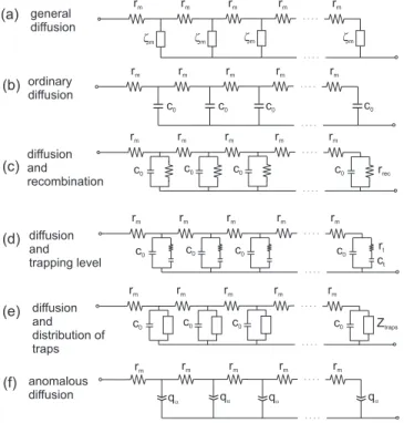
(8) PHYSICAL REVIEW B 77, 235203 共2008兲. JUAN BISQUERT. 7 and references therein兲 has not been scanned in search of trap dynamics, very probably due to the lack of suitable models that expose the frequency response of the trap distribution. It is also likely that the dynamics of electronic traps is far too fast to be observed in the usual frequency range of impedance spectroscopy 共0.1 Hz–1 kHz兲. In the case of ionic solid conductors, such as electrochromic and Li battery materials, the trap dynamics is generally much slower and more likely to be clearly detected. So one important point in the following model is to justify the appearance of anomalous diffusion in the case of the exponential distribution of traps. Such model was developed using formal considerations,19 and it has been found very powerful for describing electrointercalation diffusion in solids.21,42 Recently, published impedance data43 seem to realize all the features of the diffusion-trap model, including anomalous diffusion features. Another central aspect of photovoltaic applications, coupled with diffusion, is recombination, and this will also be considered below. In general, recombination means the loss of electronic carriers, by meeting another kind of carrier, as in electron-hole annihilation. In contrast to trapping process, in which the carriers are accumulated in certain localized states and can be retrieved, recombination is an irreversible process where the carriers are lost by transformation, and therefore, the free energy associated with such carriers does not contribute to energy output of the solar cell. The general situation treated in this section is illustrated in Fig. 8. Injection 共or extraction兲 of carriers causes diffusion along the extended states. While they advance, free carriers have the chance to be captured, and later released, by traps. In addition, free carriers have a possibility to be captured in recombination process. The recombination process specifically shown in Fig. 8 is the electron transfer from the metaloxide nanoparticles toward ionic species in solution 共these are depicted around their own Fermi level, the redox potential兲. This is the dominant recombination mechanism in standard liquid electrolyte DSC,1 where the I− / I−3 redox couple is normally used to regenerate the oxidized dye molecules from the counterelectrode. The concentration of electron acceptor ions is very high and is not affected by charge transfer from the semiconductor. The exponential distribution of traps has been amply applied in the studies of DSC with a liquid redox electrolyte, and it is agreed that the lifetime dependence on Fermi level is well explained by the trapping effect;10,44,45 however, these studies all used the quasistatic approximation. We should also remark that DSC can be made also with organic electronic hole conductors filling the voids of the porous network, and the interfacial charge transfer implies electron-hole recombination.46 In Secs. III A–III C we derive first the theory of impedance for diffusion trapping in spatially restricted conditions and, thereafter, the model for recombination coupled with trapping. The main point is to reveal the effects of trap dynamics on diffusion and recombination phenomena beyond the quasistatic approach that was used in previous works.24,25,45,47 A. General features of the diffusion impedance. Considering the different processes outlined in Fig. 8, we extend Eq. 共4兲 to the transport-conservation equation as follows:. ⳵ nc ⳵ nt ⳵ Jn nc =− − − . ⳵t ⳵t ⳵ x ␶0. 共41兲. In Eq. 共41兲 ␶0 is the lifetime of electrons in the extended states and Jn is the flux of free carriers at position x that relates to the gradient of concentration by Fick’s law, Jn = − D0. ⳵ nc , ⳵x. 共42兲. where D0 is the diffusion coefficient of the free electrons in extended states. The analysis of diffusion impedance models has been presented in previous papers19,48,49 and we build on those results here. The solution of Eq. 共41兲 for small ac perturbation, with a blocking boundary condition, is the general expression of the diffusion impedance in a film of thickness L, Z共s兲 = 关␨m共s兲rm兴1/2 coth兵L关␨m共s兲rm兴1/2其.. 共43兲. Here s = i␻ and rm is the transport impedance per unit length per area 共⍀ m兲, rm = AR1M /L,. 共44兲. R1M. is the macroscopic transport resistance of the film where of area A. rm is the reciprocal to the electronic conductivity ␴ n, rm = ␴−1 n .. 共45兲. The conductivity relates to the free electron diffusion coefficient as. ␴ n = C 0D 0 ,. 共46兲. where C0 is the specific chemical capacitance of the extended states48,50 defined in Eq. 共13兲. Equation 共46兲 is an expression of the Einstein relation.25 We note that the conductivity is given by. ␴n =. q 2n cD 0 , k BT. 共47兲. The element ␨m in Eq. 共43兲 adopts different forms, depending on the local processes included in the model 共trapping, recombination, etc.兲. For the interpretation of the model, it is useful to represent Eq. 共43兲 as a distributed equivalent circuit 共a transmission line兲. The general impedance in Eq. 共43兲 is represented in Fig. 9共a兲, and the transmission lines 共b兲–共f兲 represent specific models that will be discussed in this section. Note that Fig. 9共a兲 must be regarded as a continuous model in which the branching does not correspond to finite distances. The elements rm, associated with diffusive transport,50 are distributed in the spatial direction and are continuously interrupted by transversal elements ␨m. This combination corresponds to the physical probabilities for electronic events in Fig. 8 and gives rise to the characteristic structure of a transmission line. Generally, linear equations for physical quantities varying in space with local dissipation are represented with transmission lines, for example, acoustic waves.51 We discuss first the simplest 共ordinary兲 diffusion model, with no traps and no recombination, shown in Fig. 9共b兲. In. 235203-8.

(9) PHYSICAL REVIEW B 77, 235203 共2008兲. BEYOND THE QUASISTATIC APPROXIMATION:… rm. (a) general. rm. rm. rm. rm. 40. 300. c0 rm. rm. rm. c0 rm. rm c0. c0. rm. rm. rm. 20. 10. diffusion. (c) and. recombination. c0. c0. c0. c0. rm diffusion and distribution of traps. c0. c0 rm. c0 rm. c0. c0. c0. rm. rm. rm. rm. qa. qa. Ztraps. 10 (d). 20. 共48兲. Here, C0M is the macroscopic chemical capacitance of the film. Equation 共43兲 gives 共49兲. The characteristic transport frequency ␻d0 is the reciprocal of the transit time through the layer of thickness L,. rrec . 1 + s/␻rec. The characteristic frequency of recombination is. 共51兲. 0 0. 10. 20. 0. 5. Z' (kΩ). 10. Z' (kΩ). FIG. 10. 共Color online兲 Representation of diffusionrecombination impedance of a film of thickness L. 共a兲 Diffusion in the absence of recombination. The square point marks the angular frequency of turnover, related to ␻d = 100 rad s−1. 关共b兲,共c兲 and 共d兲兴 Diffusion-recombination impedance, showing two cases with different values of lifetime, as indicated. The yellow round point marks −1 the effective lifetime frequency ␶−1 s and 0 , with the values ␶0 = 10 ␶0 = 10−3 s. The parameters used in the calculation: T = 300 K, EF = 0.75 eV, Ec = 1 eV, Nc = 1018 cm−3, D0 = 10−4 cm2 s−1, L = 10−3 cm, and A = 1 cm2.. ␻rec0 = ␶−1 0 ,. 共52兲. and the distributed recombination resistance is given by. 共50兲. The impedance spectrum of blocked diffusion is shown in Fig. 10共a兲. At high frequencies the spectrum exhibits the 45° line 共Warburg impedance兲 associated with diffusion. At frequencies lower than ␻d0 the spectrum is capacitive, and the low-frequency resistance is R1M / 3. This is an important feature, since the electronic conductivity of the semiconductor layer can be directly extracted from R1M , by Eqs. 共44兲 and 共45兲. For diffusion and recombination, there appears a recombination resistance in parallel with the chemical capacitance in the transmission line 关see Fig. 9共c兲 and Ref. 48兴. This will be further discussed in Sec. III C. The transverse ␨ impedance in this case is. ␨m =. 5. 10. −1 this model the distributed admittance ␨m consists on the chemical capacitance. 1 D0 ␻d0 = 2 = M M . L R1 C0. 300. qa. FIG. 9. 共a兲 Transmission line representation of the diffusion impedance with the distributed diffusion resistance rn and the general transverse element ␨n. 关共b兲–共f兲兴 Specific models are indicated, depending on the local electronic processes coupled with diffusion.. Z共s兲 = R1M 共␻d0/s兲1/2 coth关共s/␻d0兲1/2兴.. 200. Z' (kΩ). 0. ␨m−1 = C0s = 共C0M /AL兲s.. 100. 30. rm. qa. 0. (c). (f) anomalous diffusion. 20. 40. rt ct. rm c0. 100. Z' (kΩ). rm c0. rm. 10. -Z'' (kΩ). and trapping level. rm. -Z'' (kΩ). (d) diffusion. rm. ωrec = 1/τ0. 0 0. rm. 200. 2π ωd. rrec 0. rm. τo = 0.001 s. 30. -Z'' (kΩ). rm. τ0 = 0.1 s. zm. -Z'' (kΩ). rm. diffusion. zm. zm. zm. (b) ordinary. (e). (b). (a). diffusion. rrec =. ␶0 = LAR3M , C0. 共53兲. where R3M is the macroscopic recombination resistance of the layer. In contrast with Fig. 10共a兲, the spectra of diffusion recombination, shown in Figs. 10共b兲–10共d兲, are resistive at low frequencies. There are two competing processes now, the transport across the layer 共␻d0兲 and the carrier loss by recombination 共␻rec0兲. The shape of the spectra is regulated by the factor relating the characteristic frequencies, which can be expressed in several alternative ways,48. 冉冊. ␻d0 R3M Ln = M= ␻rec0 R1 L. 2. ,. 共54兲. where Ln = 冑D0␶0 is the electron diffusion length. In the case of low recombination 共␻rec0 Ⰶ ␻d0 or Ln Ⰷ L兲, the carriers have plenty of time to cross the layer before they are lost. The spectrum is a recombination arc, shown in Fig. 10共b兲, and further discussed below. The diffusion Warburg is a. 235203-9.

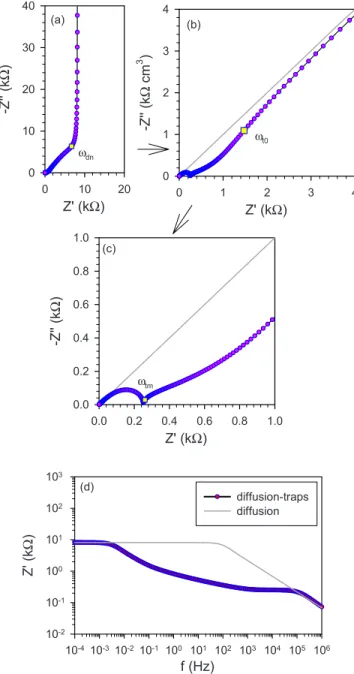
(10) PHYSICAL REVIEW B 77, 235203 共2008兲. JUAN BISQUERT 40. 3. 3. -Z'' (kΩ cm ). 20. 10. 2 ωt0. 1. ωdn 0. 0 0. 10. 20. 0. 1. Z' (kΩ) 1.0. 2. 3. 4. Z' (kΩ). (c). -Z'' (kΩ). 0.8. The calculation of the impedance of diffusion and trapping is given in Ref. 49 for a single trap. The result is that the transverse element in Eq. 共43兲 takes the form. 0.6 0.4 0.2. 共55兲. ωtm. 0.0 0.0. 0.2. 0.4. 0.6. 0.8. 1.0. Z' (kΩ) 103. (d). diffusion-traps diffusion. 102. Z' (kΩ). The resulting transmission line is shown in Fig. 9共d兲. According to Eq. 共55兲, the RC circuit of the trap is connected in parallel to the capacitance C0 of the extended states. Of interest here is the diffusion-trap impedance for an exponential distribution of localized states. It can be easily shown that the ac impedance, obtained using Eqs. 共41兲 and ⴱ is the full 共5兲, has the form of Eq. 共55兲, where now, Ctraps capacitance of the distribution 关Eq. 共18兲兴, which we have characterized in Sec. II. The distributed equivalent circuit is shown in Fig. 9共e兲, where the transverse element should be regarded as that given in Fig. 3. So we can readily calculate the shape of the spectra by including Eq. 共55兲 in Eq. 共43兲. A first set of results is shown in Fig. 11. In this example, the lowest trap frequency ␻t0 is larger than the frequency of transit time ␻dn. Therefore, the overall shape of the impedance spectra, shown in Fig. 11共a兲, is the same as that of diffusion without traps, shown in Fig. 10共a兲. The kinetic effect of trapping appears as a modification of the Warburg domain, at high frequencies, shown in Figs. 11共b兲 and 11共c兲. We find two interesting features in this high-frequency range. First, at the highest frequencies, Fig. 11共c兲, we observe the Gerischer impedance, associated with diffusion recombination, and shown before in Fig. 10共d兲. This, in fact, occurs at frequencies higher than ␻tm, which is for the fastest trap, i.e., the upper cutoff frequency of the distribution. The appearance of the Gerischer impedance is due to the fact that above ␻tm, the trap capacitors are shunted, hence the trap behaves like a pure resistance, and the circuit in Fig. 9共d兲 reduces to that in Fig. 9共c兲. In the intermediate frequency range 共␻ ⬍ ␻tm兲, we observe in Fig. 11共c兲 a diffusion line with slope lower than 45°. This indicates the occurrence of anomalous diffusion,19 and this is caused by the reduction of Ztraps to a CPE, as pointed out in Fig. 3 and discussed in Sec. II F. The CPE replaces the pure capacitance C0 of ordinary diffusion, and the transmission. (b). 30. B. Diffusion-trapping impedance. ⴱ ␨m−1 = 关C0 + Ctraps 共s兲兴s.. 4. (a). -Z'' (kΩ). small feature in the high-frequency part, clearly visible in the enlarged plot of Fig. 10共c兲, where we can see the start of the curvature of the capacitive part of Fig. 10共a兲, due to recombination. In the spectrum of Fig. 10共c兲 we can still determine the electronic conductivity from R1M / 3, i.e., the resistance at the turnover, and this method has been effectively applied in experiments.7,52 On the other hand, in the case of strong recombination 共␻rec0 Ⰷ ␻d0 or Ln Ⰶ L兲 the injected carriers penetrate a restricted extent in the layer, and the boundary condition is irrelevant. The recombination resistance distorts the diffusion spectrum even at frequencies higher than the frequency of turnover ␻d0, and the spectrum adopts the form of the Gerischer impedance, shown more clearly in Fig. 10共d兲, which corresponds to diffusion recombination in semiinfinite space.. 101 100 10-1 10-2 10-4 10-3 10-2 10-1 100 101 102 103 104 105 106. f (Hz) FIG. 11. 共Color online兲 Representation of the impedance of diffusion in a film of thickness L, with an exponential distribution of traps. 关共a兲–共c兲兴 Impedance spectra in the complex plane. The gray thin line is the impedance of diffusion without traps. The yellow square points mark the diffusion frequency ␻dn = 共C0 / Ctraps兲␻d0, the cutoff frequency ␻tm, and the deep traps frequency ␻t0. 共d兲 The real part of the impedance as a function of the frequency. The parameters used in the calculation: T = 300 K, EF = 0.75 eV, Ec = 1 eV, T0 = 1000 K 共␣ = 0.33兲, Nc = 1018 cm−3, Nt = 1020 cm−3, D0 = 10−4 cm2 s−1, L = 10−3 cm, and A = 1 cm2.. line of Fig. 9共e兲 adopts, in a restricted frequency range, the form of Fig. 9共f兲, which is the anomalous diffusion model.19,53 Let us return to the global spectrum shown in Fig. 10共a兲. Although it has the form of ordinary diffusion, as already commented, there is a strong change of the characteristic frequency of turnover, ␻dn, with respect to that of free diffusion, ␻d0. This is clearly appreciated in the representation of the impedance as a function of the frequency 关Fig. 11共d兲兴,. 235203-10.

(11) PHYSICAL REVIEW B 77, 235203 共2008兲. BEYOND THE QUASISTATIC APPROXIMATION:…. ␻dn =. 1 Dn . M M 2 = L R1共C0 + Ctraps 兲. 100. 共56兲. 0. 15. 10 ωtm. 5. 0 0. 20. 40. 0. 5. Z' (kΩ) 103. 共57兲 Z' (kΩ). 10. 15. 20. Z' (kΩ). (c). diffusion-traps diffusion. 102 101 100. 共58兲. Equation 共58兲 corresponds to the generalized Einstein relation.25 These results are an application of the quasistatic approximation24 that was mentioned in Sec. I. If the trapping dynamics is fast, then the system can be described in terms of the transport model of the trap-free system. There is a modification of the measured time constant, i.e., the chemical diffusion coefficient, which is reduced by the additional capacitance of the traps. However, the dc quantities, such as the dc conductivity, are not modified at all.25 In Fig. 12 we plot the impedance of diffusion trapping with another set of parameters and we obtain a very different result. The change is due to the fact that trapping kinetics, in this case, are slower than the transit time. Thus, the shape of spectra 关Fig. 12共a兲兴 is not that of diffusion, but instead, we obtain the impedance response of the exponential distribution of traps, shown in Figs. 5 and 7. As before, at high frequency we obtain the Gerischer impedance, which is the manifestation of diffusion trapping. In Fig. 12共c兲 we observe that the low-frequency resistance is mainly due to traps in this case and not associated to the transport resistance. Therefore, the quasistatic approximation is invalid in this case, and we cannot infer the conductivity from the lowfrequency resistance, in contrast with the previous example.. (b). 3. 40 20. In general, Dn can be interpreted as a chemical diffusion coefficient.25,47 Note that the measured conductivity 共from R1兲 is not modified, since ␴n is the same as that in Eq. 共46兲,. ␴n = CnDn = 共C0 + Ctraps兲Dn = C0D0 .. -Z'' (kΩ cm ). 60. Comparing with Eq. 共50兲, we observe that the measured diffusion coefficient in the presence of traps is C0 D0 . Dn = C0 + Ctraps. 20. (a). 80. -Z'' (kΩ). where both models are shown, for diffusion with and without traps. Here it is seen that the frequency of turnover is lowered by five decades of frequency. The reason for this is that, even though the trap relaxation occurs only at high frequencies, the traps strongly increase the equilibrium capacitance in the low-frequency range, which is given by Ctraps 关Eq. 共27兲兴, as mentioned in Sec. II D. Therefore, the turnover frequency from the Warburg to the capacitive part has the value. 10-1 10-5 10-4 10-3 10-2 10-1 100 101 102 103 104. f (Hz). FIG. 12. 共Color online兲 Representation of the impedance of diffusion in a film of thickness L, with an exponential distribution of traps. 共a兲 and 共b兲 show the impedance in the complex plane. The gray thin line is the impedance of diffusion without traps. The yellow square point marks the cutoff frequency ␻tm. 共c兲 shows the real part of the impedance as a function of the frequency. The parameters used in the calculation: T = 300 K, EF = 0.75 eV, Ec = 1 eV, T0 = 1000 K 共␣ = 0.33兲, Nc = 1018 cm−3, Nt = 1020 cm−3, D0 = 10−4 cm2 s−1, L = 10−3 cm, and A = 1 cm2.. the DOS, related to both the extended states and exponential distribution. In order to show this, we consider that diffusive transport is very fast in the system of Fig. 8. This implies that carrier densities are homogeneous. Integrating Eq. 共41兲 between the extracting boundary at x = 0 and the blocking boundary at x = L, we obtain. ⳵ nc ⳵ nt nc Jn0 =− − + . ⳵t ⳵ t ␶0 L. 共59兲. For a small perturbation in the frequency domain, Eq. 共59兲 gives. C. Trapping-recombination impedance. From previous general analysis of the impedance of solar cells, we know that recombination introduces a resistance in parallel to the chemical capacitance.54 This has been already remarked above in Fig. 10共b兲. In the case in which the diffusion transit time, L2 / D0, is much faster than the electron lifetime ␶0, the impedance response is basically given by a recombination arc. In the following, we wish to calculate the modifications of the recombination impedance by the effect of the exponential distribution of traps. The result we expect is a resistance in parallel with the full capacitance Cⴱ共␻兲 of. i␻共n̂c + n̂t兲 +. n̂c Ĵn0 . = ␶0 L. 共60兲. Using Eq. 共20兲, we can write Eq. 共60兲 as. 再. ⴱ i␻关C0 + Ctraps 共␻兲兴 +. 冎. 1 Ĵn0 , V̂ = rrec L. 共61兲. where the recombination resistance is defined in Eq. 共51兲. The impedance of the film, per unit area, is. 235203-11.

(12) PHYSICAL REVIEW B 77, 235203 共2008兲. JUAN BISQUERT. 0.3. 共62兲. 0.2 3. qĴn0. 1 rrec . = ⴱ L 1 + i␻rrec关C0 + Ctraps 共␻兲兴. -Z'' L (MΩ cm ). Z=. V̂. This shows, as anticipated, that recombination introduces the resistance rrec in parallel to the total frequency-dependent capacitance Cⴱ共␻兲 of Eq. 共17兲. Let us assume that the frequencies of the measurement are lower than the frequency ␻t0. In this case Eq. 共20兲 reduces to Ctraps n̂c , n̂t = C0. 1 rrec , L 1 + i␻␶n. C0 + Ctraps ␶0 . C0. 3. -Z'' L (kΩ cm ). 共64兲. 3. 共65兲. Equation 共64兲 means that if ␻ Ⰶ ␻t0 the relaxation dynamics is the same as that of free electrons.54 There are no kinetic effects of traps. The traps, however, modify the time constant for recombination by the ratio of equilibrium capacitances 关Eq. 共66兲兴. This is because displacing the Fermi level requires to discharge the traps, as was first noted by Rose.22,23 The quasistatic approximation considerably simplifies the analysis of experimental techniques that probe the properties of DSC; see, for example, Refs. 10 and 45 that discuss the experimental determination of Eq. 共66兲. In Fig. 13 we have plotted the impedance of the exponential distribution of traps with the parallel recombination resistance 关Eq. 共62兲兴. We have neglected the free charge capacitance C0 since this is usually not significant in ⴱ , unless EF is very close to the comparison to Ctraps conduction-band edge. Now there are two characteristic frequencies in the system: ␻t0 indicates the onset of trap relaxation and CPE behavior, as discussed above, and ␻rec = ␶−1 n is the effective lifetime frequency. In Fig. 13共a兲 we have ␻t0 Ⰷ ␻rec, therefore the traps relaxation discussed in Fig. 7, occurs undisturbed at very high frequencies. When lowering the frequency, the impedance closes toward the real axis by the effect of recombination resistance, as in Fig. 10共b兲. The recombination arc54 has the characteristic frequency ␶−1 n . In Fig. 13共b兲 we have still ␻t0 ⬎ ␻rec, but their values are closer than in the previous example, and in this case the trap. 0.1. 0. 100. 5. 10. 15. 20. Z' L (MΩ cm3). 10. (b). 50 ωt0. 0. ωrec. 0. 10. 20. 0. 10. 50. 100. 150. 200. Z' L (kΩ cm3). (c). Qshallow ωt0. 5 ωrec. 0 0. 共66兲. 0.0 0.0. 0. where, by Eq. 共53兲,. ␶n =. ωrec. 20. and this can be written Z=. ωt0. 0.1. 共63兲. -Z'' L (kΩ cm ). 1 rrec , L 1 + i␻rrec关C0 + Ctraps兴. (a). 0. where Ctraps is given in Eq. 共27兲. Equation 共63兲 is the rigorous formulation of the quasistatic approximation24 for small modulation quantities. It means that the modulation of the trapped charge follows instantaneously the modulation of the free charge, as mentioned before, and the ratio of these quantities is given by equilibrium chemical capacitances of the corresponding states. If Eq. 共63兲 holds, then from Eq. 共62兲 we arrive at the impedance Z=. 10. 5. 10. 15. Z' L (kΩ cm3). 20. FIG. 13. 共Color online兲 Repesentation of impedance of a film of thickness L, with an exponential distribution of traps with recombination from the conduction band. The green square point marks the deep trap frequency ␻t0, and the blue round point marks the effective lifetime frequency ␶−1 n , with the values 共a兲 ␶0 = 1 s and ␶n = 362 s, 共b兲 ␶0 = 0.01 s and ␶n = 3.62 s, and 共c兲 ␶0 = 0.001 s and ␶n = 0.362 s. In 共c兲 in green dashed line the CPE approximation at high frequency is indicated. The parameters used in the calculation: T = 300 K, EF = 0.4 eV, Ec = 1 eV, T0 = 800 K 共␣ = 0.375兲, Nc = 1020 cm−3, Nt = 1020 cm−3, and ␤ = 10−10 cm2 s−1.. relaxation is visible as a modification of the recombination arc in the high-frequency part. Finally, in Fig. 13共c兲, we have ␻t0 ⬍ ␻rec. In this case the recombination resistance is smaller than the trap resistance. Therefore, the CPE behavior of trap relaxation is fully visible and is converted into an arc at the lower frequencies by the parallel recombination resistance. It should be recalled that Fig. 13 represents a homogeneous model of recombination, in which carrier transport is infinitely fast, as assumed above. The impedance patterns of Fig. 13 are remarkably similar to those of the diffusionrecombination impedance in Figs. 10共b兲 and 10共c兲. In principle, this similarity introduces an ambiguity of models that could lead to mistake interpretation of trapping recombination 共or trapping reaction兲 as diffusion-recombination results. However, from the Fermi-level dependence of the resistance in the high-frequency straight part, both models, diffusion and traps, should be readily distinguished. Indeed, in the diffusion model the high-frequency feature gives the transport. 235203-12.

(13) PHYSICAL REVIEW B 77, 235203 共2008兲. BEYOND THE QUASISTATIC APPROXIMATION:… 1.0. -C'' /Ctot. resistance R1, which depends on the potential as exp关共Ec − EF兲 / kBT兴关Eq. 共47兲兴. In contrast, the Fermi-level dependence of the traps resistance is much more steep, as indicated in Eq. 共33兲 and in Fig. 6共b兲. Therefore, we should emphasize that the spectra should be monitored over a sufficient variation of bias potential in order to determine the correct interpretation. In experimental results of impedance of DSC, the mentioned transport resistance dependence of Fermi level was observed,7,55 it therefore appears that trap relaxation is quite fast in nanostructured TiO2 surrounded with liquid electrolyte, and the widespread application of the quasistatic approximation is well justified. The extension of the approach presented in this section, for nonhomogeneous device models, requires a twofold numerical solution. First, steady-state equations must be solved to find the local values of charge density at each point of the device. Then, such information allows us to write the transport equations for small ac quantities, which contain also dc parameters. An example is given in Ref. 50.. 0.6. ωt2. 0.4. ω. 0.0 0.0. 0.2. ACKNOWLEDGMENTS. The work was supported by MEC under Project No. MAT2007-62982, HOPE Project No. under Grant No. CSD2007-00007 共Consolider-Ingenio 2010兲, and Generalitat Valenciana under Project No. ACOMP07/103. I am grateful to Henk Bolink for discussions on organic conductors.. 0.6. 0.8. 1.0. (b). -Z'' (kΩ ). 1.0 ω. 0.0 0.0. 0.5. 1.0. 1.5. 2.0. Z' (kΩ ). FIG. 14. 共Color online兲 Representation of 共a兲 capacitance and 共b兲 impedance in the complex plane, for single and double trap models, as indicated. Parameters: Ct1 = 10−3 F, Rt1 = 103 ⍀, ␻t1 = 1 rad s−1, Ct1 = 5 ⫻ 10−3 F, Rt1 = 2 ⫻ 103 ⍀, ␻t1 = 0.1 rad s−1, and Ctot = Ct1 + Ct2.. Here, Ct1 is the trap capacitance and ␻t1 is a constant, the characteristic trap frequency. The impedance associated with Eq. 共A1兲 is Zt1共␻兲 = Rt1 +. 1 , i␻Ct1. 共A2兲. where the trap resistance is defined as. Rt1 =. 1 . ␻t1Ct1. 共A3兲. From Eq. 共A2兲 we see that the equivalent circuit of the trap is RC series. In the complex plane the capacitance forms an arc, of width Ct1, while impedance forms a vertical line, being the resistance constant at all frequencies. This is illustrated in Fig. 14. When we combine two traps, the RC circuits are in parallel, as indicated in Fig. 1, so we have ⴱ 共␻兲 = Ctot. 共A1兲. C' /C. 1.5. APPENDIX: IMPEDANCE AND CAPACITANCE OF SIMPLE COMBINATIONS OF TRAPS. The frequency-dependent capacitance of a single trap is. 0.4. tot. 2.0. 0.5. The relaxation of an exponential distribution of traps in the frequency domain contains two main features. At low frequency the distribution gives the normal relaxation of a single trap, i.e., a RC series circuit. At high frequency the distribution responds as a constant-phase element. The CPE exponent is independent of the Fermi-level position but changes with the temperature as ␣ = T / T0. The transition between the two features occurs roughly at the frequency of the highest occupied trap level at the position of the Fermi level. In the presence of diffusion and recombination, the interplay between the frequency of the highest occupied trap level and the effective 共chemical兲 diffusion coefficient or effective lifetime determines the shape of impedance spectra. In the presence of very slow traps, the quasistatic approximation is not valid, since the low-frequency response is governed by the trap kinetics. We have found similarities between diffusionrecombination and trapping-recombination impedance models. Therefore, a careful analysis of experimental data is necessary, regarding these models, and exploring a wide window of potential and if possible temperature seems recommended to identify correctly the trap relaxation by impedance spectroscopy. The variation of impedance parameters with bias potential and temperature in agreement with the model should provide strong evidence for the identification of the trap kinetics.. Ct1 = . 1 + i␻/␻t1. one trap two traps ωt1. (a). 0.2. IV. CONCLUSIONS. ⴱ 共␻兲 Ct1. 0.8. Ct1 Ct2 + . 1 + i␻/␻t1 1 + i␻/␻t2. 共A4兲. This forms a double arc in the complex capacitance plane, as shown in Fig. 14共a兲. If we calculate the real part of the ⴱ , we obtain impedance, Ztot = 1 / i␻Ctot. 235203-13.

(14) PHYSICAL REVIEW B 77, 235203 共2008兲. JUAN BISQUERT. Re关Ztot共␻兲兴 =. 2 2 Rt1Rt2关Rt1␻t1 + Rt2␻t2 + 共Rt1 + Rt2兲␻2兴 . 2 共Rt1␻t1 + Rt2␻t2兲 + 共Rt1 + Rt2兲2␻2. 共A5兲. because the impedances of the capacitors vanish at high frequency. On the other hand, the low-frequency limit of the real part of the impedance depends on the capacitances 共via the characteristic frequencies兲,. In the high-frequency limit this gives Re关Ztot共␻ → ⬁兲兴 =. Rt1Rt2 . Rt1 + Rt2. 共A6兲. Therefore, the impedance intersects the x axis at the value of the parallel combination of the trap resistances. This is. O’ Regan and M. Grätzel, Nature 共London兲 353, 737 共1991兲. 2 J. Bisquert, D. Cahen, S. Rühle, G. Hodes, and A. Zaban, J. Phys. Chem. B 108, 8106 共2004兲. 3 C. J. Brabec, N. S. Sariciftci, and J. C. Hummelen, Adv. Math. 11, 15 共2001兲. 4 P. Peumans, U. Uchida, and S. R. Forrest, Nature 共London兲 425, 158 共2003兲. 5 J. H. Burroughes, D. D. C. Bradley, A. R. Brown, R. N. Marks, K. MacKay, R. H. Friend, P. L. Burn, and A. B. Holmes, Nature 共London兲 347, 539 共1990兲. 6 S. R. Forrest, Nature 共London兲 428, 911 共2004兲. 7 Q. Wang, S. Ito, M. Grätzel, F. Fabregat-Santiago, I. Mora-Seró, J. Bisquert, T. Bosshoa, and H. Imai, J. Phys. Chem. B 110, 19406 共2006兲. 8 B. Ramachandhran, H. G. A. Huizing, and R. Coehoorn, Phys. Rev. B 73, 233306 共2006兲. 9 J. Bisquert, Phys. Chem. Chem. Phys. 10, 49 共2008兲. 10 L. M. Peter, J. Phys. Chem. C 111, 6601 共2007兲. 11 M. C. J. M. Vissenberg and M. Matters, Phys. Rev. B 57, 12964 共1998兲. 12 P. Servati, A. Nathan, and G. A. J. Amaratunga, Phys. Rev. B 74, 245210 共2006兲. 13 G. Paasch and S. Scheinert, J. Appl. Phys. 101, 024514 共2007兲. 14 M. M. Mandoc, B. de Boer, G. Paasch, and P. W. M. Blom, Phys. Rev. B 75, 193202 共2007兲. 15 Z. Chiguvare and V. Dyakonov, Phys. Rev. B 70, 235207 共2004兲. 16 M. D. Levi and D. Aurbach, J. Phys. Chem. B 109, 2763 共2005兲. 17 J. Bisquert, Phys. Chem. Chem. Phys. 5, 5360 共2003兲. 18 J. Bisquert, F. Fabregat-Santiago, I. Mora-Seró, G. GarciaBelmonte, E. M. Barea, and E. Palomares, Inorg. Chim. Acta 361, 684 共2008兲. 19 J. Bisquert and A. Compte, J. Electroanal. Chem. 499, 112 共2001兲. 20 J.-W. Lee and S.-I. Pyun, Electrochim. Acta 50, 1777 共2005兲. 21 C. Montella, R. Michel, and J. P. Diard, J. Electroanal. Chem. 608, 37 共2007兲. 22 A. Rose, RAC Rev. 12, 362 共1951兲. 23 A. Rose, Concepts in Photoconductivity and Allied Problems 共Interscience, New York, 1963兲. 24 J. Bisquert and V. S. Vikhrenko, J. Phys. Chem. B 108, 2313 共2004兲. 25 J. Bisquert, Phys. Chem. Chem. Phys. 共to be published 2008兲.. 2 2 Rt1␻t1 + Rt2␻t2 . 共Rt1␻t1 + Rt2␻t2兲2. 共A7兲. The impedance rises vertically when the frequency decreases, but it makes a transition between the values in Eqs. 共A6兲 and 共A7兲关see Fig. 14共b兲兴.. 26 L.. *bisquert@fca.uji.es 1 B.. Re关Ztot共0兲兴 = Rt1Rt2. M. Peter, A. B. Walker, G. Boschloo, and A. Hagfeldt, J. Phys. Chem. B 110, 13694 共2006兲. 27 M. E. Gershenson, V. Podzorov, and A. F. Morpurgo, Rev. Mod. Phys. 78, 973 共2006兲. 28 J. Orenstein and M. Kastner, Phys. Rev. Lett. 46, 1421 共1981兲. 29 T. Tiedje and A. Rose, Solid State Commun. 37, 49 共1981兲. 30 A. L. Roest, P. E. de Jongh, and D. Vanmaekelbergh, Phys. Rev. B 62, 16926 共2000兲. 31 D. L. Loose, J. Appl. Phys. 46, 2204 共1975兲. 32 F. Fabregat-Santiago, I. Mora-Seró, G. Garcia-Belmonte, and J. Bisquert, J. Phys. Chem. B 107, 758 共2003兲. 33 J. Jamnik and J. Maier, Phys. Chem. Chem. Phys. 3, 1668 共2001兲. 34 C.-T. Sah, Fundamentals of Solid State Electronics 共World Scientific, Singapore, 1991兲. 35 C. E. D. Chidsey and R. W. Murray, J. Phys. Chem. 90, 1479 共1986兲. 36 J. Bisquert, Electrochim. Acta 47, 2435 共2002兲. 37 H. Bässler, Phys. Status Solidi B 175, 15 共1993兲. 38 J. G. Simmons and G. W. Taylor, Phys. Rev. B 4, 502 共1971兲. 39 I. Mora-Seró and J. Bisquert, Nano Lett. 3, 945 共2003兲. 40 T. Dittrich, I. Mora-Seró, G. Garcia-Belmonte, and J. Bisquert, Phys. Rev. B 73, 045407 共2006兲. 41 J. A. Anta, I. Mora-Seró, T. Dittrich, and J. Bisquert, J. Phys. Chem. C 111, 13997 共2007兲. 42 J. Backholm, P. Georén, and G. A. Niklasson, J. Appl. Phys. 103, 023702 共2008兲. 43 F. Bardé, P. L. Taberna, J. M. Tarascon, and M. R. Palacín, J. Power Sources 179, 830 共2008兲. 44 L. M. Peter, J. Electroanal. Chem. 599, 233 共2007兲. 45 J. Bisquert, A. Zaban, M. Greenshtein, and I. Mora-Seró, J. Am. Chem. Soc. 126, 13550 共2004兲. 46 H. J. Snaith and L. Schmidt-Mende, Adv. Math. 19, 3187 共2007兲. 47 J. Bisquert, J. Phys. Chem. B 108, 2323 共2004兲. 48 J. Bisquert, J. Phys. Chem. B 106, 325 共2002兲. 49 J. Bisquert and V. S. Vikhrenko, Electrochim. Acta 47, 3977 共2002兲. 50 A. Pitarch, G. Garcia-Belmonte, I. Mora-Seró, and J. Bisquert, Phys. Chem. Chem. Phys. 6, 2983 共2004兲. 51 L. Brioullin, Wave Propagation in Periodic Structures 共Dover, New York, 1953兲.. 235203-14.

(15) PHYSICAL REVIEW B 77, 235203 共2008兲. BEYOND THE QUASISTATIC APPROXIMATION:… 52. F. Fabregat-Santiago, G. Garcia-Belmonte, J. Bisquert, A. Zaban, and P. Salvador, J. Phys. Chem. B 106, 334 共2002兲. 53 J. Bisquert, G. Garcia-Belmonte, and A. Pitarch, ChemPhysChem 4, 287 共2003兲. 54 I. Mora-Seró, J. Bisquert, F. Fabregat-Santiago, G. GarciaBelmonte, G. Zoppi, K. Durose, Y. Proskuryakov, I. Oja, A.. Belaidi, T. Dittrich, R. Tena-Zaera, A. Katty, C. Lévy-Clement, V. Barrioz, and S. J. C. Irvine, Nano Lett. 6, 640 共2006兲. 55 F. Fabregat-Santiago, J. Bisquert, G. Garcia-Belmonte, G. Boschloo, and A. Hagfeldt, Sol. Energy Mater. Sol. Cells 87, 117 共2005兲.. 235203-15.

(16)