A Model of Artificial Genotype and Norm of Reaction in a Robotic System
12
0
0
Texto completo
(2) E. G− → P (GEP) map. For an understanding of this concept it is fundamental to consider the role of phenotype plasticity and the idea of reaction norm, which are introduced as the basic link relating the three variables (GEP). Phenotype plasticity is the property of a given genotype to produce different phenotypes in response to distinct environmental conditions. The fundamental conceptual research tool in phenotypic plasticity is the idea of norm of reaction [10]. A norm of reaction is a function that relates the environments to which a particular genotype is exposed and the phenotypes that can be produced. In practice, such a tabulation can only be made for a partial genotype, a partial phenotype, and some particular aspects of the environment [6]. Frequently, this abstraction level has been used to model evolutionary behaviors in artificial systems. The G → P map is usually the basis of bio-inspired genetic algorithms (GAs). However, such algorithms have been more concerned with imitating the evolution process results in order to solve searching and optimization problems. Genetic algorithms emphasize the use of a “genotype” that is decoded and evaluated. These genotypes are often simple data structures [14]. Genetic algorithms are a simple form of evolutionary algorithms (EAs). These are composed of four components: a genotype, G → P mapping, a set of variation operators, and a user-defined function to be optimized, called a fitness function. The EAs are often classified as “black-box optimization algorithms” [3]. Overall, this kind of algorithms propose that, although evolution manifests itself as a succession of changes in a species’ features, it is the changes in the genetic material that form the essence of evolution [13]. The main idea of these methods is based on the “genetic blueprint” or a “genetic programme”. In other words, genes determine phenotypes. This sort of answer bypasses the process of development, which is treated as an incidental blackbox with no direct causal relevance to the evolutionary process [11]. From this point of view, changes in the species are produced by isolated changes in the individuals. In addition, the influence of the environment is limited to be used merely as a testbed to evaluate the phenotype fitness. Evolutionary Robotics (ER) proposes to employ EAs to design robots or, more often, control systems for robots. Over millions of years of evolution, living organisms have adapted to different environments and have competed for survival, allowing them to improve their phenotypic attributes. From a conceptual standpoint, the information to generate living organisms has been transmitted in successive generations, improving and diversifying in each iteration and generating the particular attributes in each species. Nowadays, any species has the same common phenotype as a result of evolution because this information is transferred to the new members by inheritance. The species’ individuals have differences which are usually morphological, but the main mechanism that accounts for these allelic differences is not mutation in genes, as in clasical EAs. The aim of this paper is to propose an artificial genotype data structure which generates a given phenotype conditioned by an environment. In particular, this work is focused on the way the species share functionalities using their genes..
(3) To evaluate the performance of this proposed artificial genotype, a “species” of robotic system is used. The artificial genotype for each species’ individual is obtained and it is used to check the GEP model proposed. To do this, the reaction norm of the species’ individuals is estimated. The proposed artificial genotype shows the same behavior that a biological genotype does in relation to phenotype plasticity.. Initial functional protein params.. Θ1,2. Θ2,1. 0. Θ2,2. 0. Θn ,2. Θn ,1. Γ1. Species' regulatory parameters. ω1. GENOTYPE. Γ2. Allelic parameters. 0. 0. Θ2, m. 0. 0. Θn , m. Species' functional parameters. W1. Ω1,1. Ω2,1. Ωl ,1. W2. Ω1,2. Ω2,2. Ωl ,2. Wm. Ω1, m Ω2, m. Ωl , m. M (Y , ^ Y). Θ1,1. Θ1,2. Θ1, m. Θ2,1. Θ2,2. Θ2, m. Θn ,1. Θn ,2. Θn , m. b1. ω2. Γa. Adaptation Function. 0. Θ1, m. PHENOTYPE T. Ψ(Ω , X ) Θ. b2. ωm. Adapted functional protein params.. ^ Y. Transcription Function. X. + -. 0. +. T. Φ(ω ,b , Γ) W. 0. Θ1,1 1. +. Translation Function. bm. ENVIRONMENT Individual. Y. Species. Figure 1: Schema of the proposed genotype model and the relationship with the environment and phenotype. 2 2.1. Model Genotype model. The biochemical information stored in the DNA strings is converted in some way in living organisms with their anatomy, physiology and behaviors. In the proposed model, different types of information are defined according to the way this information is encoded in living organisms. The genotype model proposed transfers this information to a space parameters – Allelic information. It is the information stored in DNA which encode amino acids and proteins directly, so some phenotypes can be determined directly by this information. This information is encoded by allelic parameters: Γ = {Γ1 , Γ2 , ..., Γa } | Γ ∈ Ra , where a is the number of encoded allels..
(4) – Species’ regulatory information. It is related to information stored in DNA which does not encode amino acids directly, but is shared by all individuals of the species.This kind of data is encoded by the species’ regulatory parameters(SRP). There are two kind of SRP parameters: the first class is the regulatory parameters of transcription function: W = {W1 , W2 , ..., Wm , } | Wi ∈ Rt where t is the number of combinations of the encoded proteins from allelic genes, to encode a functional protein. The second class is the combination parameters from allelic and species’ regulatory information: ω = {ω1 , ω2 , ..., ωm } | ωi ∈ Ra,t , b = {b1 , b2 , ..., bn } | bi ∈ Rt . – Species’ functional information. It is the information encoded in DNA which is transformed into specific species’ phenotypes. The function of this information is regulatory and regards the control of the functional combination of synthesized proteins from allelic information which is encoded by the species’ functional parameters (SFP): Ω ∈ Rl,m , where l is the number of the environment modifiers and m is the number of proteins which adjust the obtained phenotype. – Functional protein configuration. It is a sequence of proteins that are obtained from the translation function and regulatory species information. These proteins represent a certain phenotype which can be modified by the environment. This kind of information is transferred into parametric space: initial functional protein parameters(F P P 0 ), these parameters represents the initial proteins synthesized from species’ genes, but they are going to be 0 }| modified by the interaction with the environment. Θ0 = {Θ10 , Θ20 , ..., Θm Θi0 ∈ Rn where n is the number of parameters that define a phenotype. The successive modified sets of functional parameters depend on the consecutive environments where the individual has been adapted. This kind of parameters are named adapted functional protein parameters: Θ = {Θ1 , Θ2 , ..., Θm } | Θi0 ∈ Rn where n is the number of parameters that define a phenotype. 2.2. GEP mapping model. So far, we have encoded the information stored in DNA in a parametric space. The parameter space defined above can be considered as a data structure. Several operations can be established for modeling GEP mapping (fig. 1). Hence, a species’ individual has got a genotype defined by the previous structure. One part is specific for this individual (allelic information). In the biological case, this information is represented by allelic genes which can be converted into proteins. The transcription of one gene may be turned on or off by other genes called regulatory genes [6]. In the proposed system, this transcription process is modeled by the transcription function (eq. 1). Θ0 = Φ(ω, b, Γ )T W. (1). In a mathematical way, the transcription function is a regression model that relates the allelic information with initial functional parameters. The SRP fit this model and represent the information shared with every member of this species that accounts for the phenotypic behavior..
(5) Furthermore, proteins encoded by one gene may modify the proteins encoded by a second gene in order to activate or deactivate protein function. The equivalent of the latter proteins are the SFP in the proposed model. These proteins can also be modified by the environment through signal transduction. Moreover, proteins encoded by one gene may bind to proteins from other genes to form an active complex that performs some function. This is modeled by a transduction function. Ŷ = Ψ (Ω, X)T Θ (2) This function finally generates a phenotype. From a mathematical point of view, the transduction function is a recursive regression model, where there are some input cues (X) that are combined with common fixed parameters (Ω) into a nonlinear function Ψ for all the species individuals and the regression parameters are Θ. So far, the environment adaptation has not been considered. In 1930, Ronald A. Fisher emphasized [4] that adaptation is characterized by the movement of a population towards a phenotype that best fits the present environment. However, this evolution is produced by changes in the individuals in this population. In the proposed model, this is considered in the adaptation function. Θe = Θe−1 + M (Y, Ŷ ). (3). where e is the number of interacting successive environments. This equation has to accomplish these limit restraints: when e = 0 → Θe = Θ0 and the difference between Θe − Θe−1 has to tend to zero. The value Y is the optimal phenotype and Ŷ is the current individual phenotype. Eq. 3 expresses a sequence of changes in functional proteins modifying the phenotype showed by the individual. The motor for these changes is the gap between the optimal phenotype and the current phenotype expressed in a functional way in the adaptation function. This had been defined as a first degree dynamic system where its initial condition is defined by the initial functional protein parameters. When the individual is adapted the gap between Y and Ŷ has to be minimum (Θe∗ ). Once in this point, there might be another adaptation stage for the individual, so Θe∗ generates epigenetic changes in SRP. This changes are propagated to the descendants improving Θ0 estimation. From an information point of view, the environment adaptation is a learning procedure whose goal is to learn the environment model to better predict the response to environmental cues.. 3 3.1. Case study The robot species description. Of course, the genotype for a robotic system is not defined as a biological system, but from an information point of view the model GEP can be considered valid for a robot. In this case, the environment is the part of the universe with which.
(6) the robot interacts, i.e. it receives information through its sensors and modifies it using its actuators. The phenotype comprises not only its morphology but also its behavior. The genotype as defined above is composed of the allelic information, which are the parameters or design variables of the robot, and the information concerning the species. This last point is a critical question because it is not usual to work with the concept of species in robotics. Two robots belong to the same ”species” if they have the same number of design variables and show a similar behavior in a similar environment. Let us consider a species composed of robot heads. We have selected this species because it presents sensor and actuators to interact with the environment. These sensors and actuators may be different between individuals from the same species. However, this species can show a behavior that is shared by all its individuals, namely saccadic movements. This species is characterized for having two cameras and 3 DOF. One of them for each camera and the other shared. The morphological traits can be described from a robotics point of view as a Denavit-Hartenberg model (Table 1). In addition, the sensor traits, are modeled by the pinhole scheme. So each camera has several characteristics: focal length, pixel size (supposed squared), height and width image resolution. Therefore, the design parameters, which are individual traits into the same species, are defined by a=16 values. This information corresponds to allelic information in the proposed genotype model (Γ ∈ R16 ). The genotype-phenotype mapping of this allelic information is directly the morphology and sensor properties of each individual in the species and it is not dependent on the environment. If other complex phenotypes are defined for every individual of this species, for example, the ability to execute saccadic movements, the environment must be considered. A saccade is a fast eye movement that shifts the gaze to a target point and can be used to scan the visual space [2]. We will focus on the transformation that links the visual position of a stimulus into a target position of the eyes, as well as on feedback error learning (FEL) as described in [8]. In this method, there are two inverse controllers. A fixed controller (B) that slowly drives the system toward the target and provides a learning signal to a second adaptive controller (Cf ). In this case, the phenotype is quantified by the gaze point after a saccade. If the projection of the gaze point were in the center of the two images, the phenotype would be optimal. Therefore, the gap for the adaptation function is the difference between these gaze points. 3.2. The environment. The environment is a spatial region around the robot head. A virtual object is randomly placed in the vision field of the two robot cameras. This object is static related to the robot frame. To assure that these points cam be watched by the two cameras at the same time, the environment region has been generated from the minimal and maximum tilt, version and vergence angles of the heads. For this reason the resulting region is not regular and the geometrical centroid point is used to represent this spatial region..
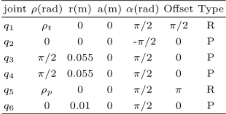
(7) Table 1: Denavit-Hartenberg model of the left side of the head. ρp , ρt are the revolute joints of the pan and common tilt motors. The right side is the same model and it shares the ρt joint. 5 z. 4 3 6. z. 0.04 y x. 3. 4. 0.06. Z5. y xX Y. Z. X. 0.02. Y 0. 1. joint ρ(rad) r(m) a(m) α(rad) Offset Type 2 2. q1. ρt. 0. 0. π/2. π/2. R. q2. 0. 0. 0. -π/2. 0. P. q3. π/2. 0.055. 0. π/2. 0. P. q4. π/2. 0.055. 0. π/2. 0. P. q5. ρp. 0. 0. π/2. π. R. q6. 0. 0.01. 0. π/2. 0. P. 3.3. X (m). 6. -0.02. 0.02 0 -0.02. Z (m). -0.04 -0.04. -0.02. 0. 0.02. 0.04. 0.06. Y (m). Figure 2: Example of the head model. Applying the GEP model to the robotic system. To match the GEP model with the robot species proposed, it is necessary to identify the transcription, activation and adaptation function. In the proposed case, to adapt the saccadic behavior to the environment, the robot must learn how it has to change the cameras position to gaze the object. The environment transduction cues are the projection of the visual stimulus in the robot camera images. They, combined with the propioception of the robot, must generate the saccadic behavior. The transduction function is really the system controller. If the robotic system had perfectly adapted to the environment, the projection of the visual point in the images of the cameras would be in the center, exactly. So the distance between the real projection to the image center could be considered as a gap between the optimal phenotype and the showed phenotype. In the GEP proposed model, the system controller represented by a transduction function is modified by an adaptation function depending on the phenotype gap, so the proposed system controller represented by a transduction function is really an adaptive controller. In the proposed FEL model [2] for one robot, there are two controllers, a fixed one (B) and adaptive (Cf ), both contributions are the system controller. As B is independent of the environment, it is possible to apply the G → P model and B can be estimated from allelic information (Γ ), directly. The Cf controller is implemented by a single-layer neural network, with 7 inputs and 3 outputs. The environment cues are defined by these seven inputs (l =7). Gaussian activations using random space features [12] were used for the hidden layer. If these random space features are the same for every species’ individual, they are the species’ functional parameters (Ω), because they regulate the phenotype function. The weights in this network combine the activation functions, as the transduction function is modified by functional proteins parameters in the proposed model, hence these weights are Θ. The dimensions of Θ are the number of units in the hidden layer (n) and the number of outputs (m). The adaptation function is.
(8) equivalent to adapt the weights in the neural network. In [2] the incremental sparse spectrum Gaussian process regression (I-SSGPR) is used. Finally, the transcription function is another regression model that relates the allelic information with the initial functional parameters (Θ0 ). Hence, the regression parameters can be obtained if Γ and Θ0 are known. The problem is to fix the Θ0 value for each individual in the species. 3.4. Getting the robot genotype. Thus, if a population of robots from the same species is forced to adapt to the same environment and to develop the same behavior, the shared information that defines the behavior of all the species individuals can be extracted. To do this: 1. A robot population is generated, changing their allelic information. The SRP and F P P 0 are initialized randomly but they are the same for all the members of the species. 2. Each individual is immersed into the same environment and it is forced to adapt to get Θe∗ from (eq. 3): dM (Y, Ŷ ) ≈ 0 → Θe = Θe∗ de. (4). 3. With the Θe∗ value for each individual and their allelic information, the transcription function is converted into a regression problem where its parameters are the SRP. A fixed environment is used to obtain these parameters. The species individuals will adapt quickly in similar environments and slowlier in different ones. Prismatic joints (cm) Left size p Γi,1 p Γi,3 p Γi,5 p Γi,7. = q2 = q3 = q4 = q6. Right side. ∈ [−0.054, 0.054] ∈ [0, 0.07] ∈ [−0.02, 0.054] ∈ [0, 0.01]. Cameras parameters:. p Γi,2 p Γi,4 p Γi,6 p Γi,8. = q2 = q3 = q4 = q6. p = Γi,1 + [0, 0.01] p = Γi,3 + [0.035, 0.07] p = Γi,5 + [0, 0.02] p = Γi,7 + [0, 0.01]. f (px); s(m/px);w (px);h(px). Left camera. Right camera. p Γi,9 = fl ∈ [340, 1920] p Γi,11 = sl ∈ [3. 10−6 , 7. 10−6 ] p Γi,13 = hl ∈ [340, 1920] p Γi,15 = wl ∈ [340, 1920]. p Γi,10 p Γi,12 p Γi,14 p Γi,16. p = fr = Γi,9 + [0, 200] = sr ∈ [3. 10−6 , 7. 10−6 ] p = hr = Γi,13 + [0, 200] p = wr = Γi,15 + [0, 200]. p p p p p p p p if Γi,13 > Γi,15 , swap(Γi,13 , Γi,15 ) if Γi,14 > Γi,16 , swap(Γi,14 , Γi,16 ). Table 2: Design parameters to generate the allelic information.
(9) 4. Experimental results. To validate the model fitting to a population of robots, the shared information by every individual of this population must be known. In the living organism, this information is encoded in DNA, but in robots, we have to set up an environment, a behavior and an allelic encoded morphology for each individual in order to get that shared information. Once we have the species genotype model, we must check if this model shows the same performance that the living organisms. That is, when an individual’s genotype is completely defined and it is placed in different environments, the phenotype has to be changed according to the norm of reaction. 4.1. Generating a population of robots. A robot model was used to simulate different robot head setups (44271 individuals were generated ) with allelic information as described in the previous section. A reasonable interval is fixed to avoid unfeasible configurations. The values of the left side of the head are chosen randomly and the right side is defined in a random interval as shown in Table 2. The generated population is split into three groups: (i) Adaptation group (26500 individuals). This group is used to get an estimation of the transcription function because there is no knowledge about the species regulatory parameters. (ii) Control group (4500 individuals). This group is used to validate the species regulatory parameters obtained from the adaptation group. (iii) Control population (13271 individuals). This group is used to validate the obtained genotype. 4.2. Getting the genotype model from the generated population of robots. Each of the individuals in the adaptation group, that were generated previously, is immersed in the same environment and it starts the adaptation process interacting with this environment. The F P P 0 are zero for all individuals because there is no previous information. The SFP are randomly initialized, however they are shared by all the species individuals. Hence, all of them show the same initial degree of adaptation to this environment. The result of this adaptation process is a set of pairs of allelic information (Γ ) and Θc∗ (eq. 4). From a robotics point of view, the used neural network controller has the same value for the initial weights (zero) for all training cases. In addition, a unique set of random sparse features are generated for all neural network controllers. Each robot setup is trained with the same environment using the same neural network parameters tuned previously [5]: variance of the model (σn2 =0.1), signal variance (σf2 =1.0) and number of projections (m=300) so the number of neural centers is 600. With these parameters the mathematical dimensions of the proposed genotype are defined as: Γ ∈ R16 and Ω ∈ R3,300 . The F P P 0 are Θ ∈ R3,600 . The results of this process are the neural network weights for.
(10) each robotic head setup that allow the robot head to generate saccadic movements. In figure 3a, there is an example of how the phenotype changes with each adaptation. The relationship between the allelic and the species’ regulat-. Norm of reaction. 9 R 2 =0.9664. Example of adaptation curve. 24. 8. 22. 7. Phenotype (px). 20. phenotype (px). 18 16 14. R 2 =0.9003 6. 5 R 2 =0.9369. 12. 4 10 8. 3. 6. 2. 4 0. 50. 100. 150. 200. 250. 300. 350. 400. 450. 500. 0. 0.1. 0.2. 0.3. 0.4. 0.5. 0.6. 0.7. Environment (m). iterations. (a) Example of adaptation curve. (b) Norm of reaction. Figure 3. ory information connect the particular traits of an individual with specific traits of the species. After the environment adaption described previously, a set of allelic information, and species’ functional parameters are defined along with a valid set of initial functional protein parameters for each individual. As it is shown in (eq. 1), the transcription function is a regression model. Hence, it is possible to use any regression method to estimate the parameters (ω, b, Γ ). The challenge is to solve the dimensional problem. In particular, the mapping from Γ (16 dimensions) to Θ (1800 dimensions). Fortunately, due to the fact that the weights of a trained network are independent among them, the regression problem can be decomposed into multiple smaller regression problems. Each Θi is influenced by Γ independently of the rest of Γ . The problem is transformed into solving 1800=(3x600 dimensions of Θ) small regression problems. In this way, the SRP are the set of parameters of each regression. The regression tool used is a MLP neural network with 16 inputs, 10 units in the hidden layer and one output. The hyperbolic tangent function was used for the hidden layer and the output layer was linear. The algorithm to train each network was the scaled conjugate gradient descent (SCG) [9]. The performance follows from comparing the weights obtained after training the adaptive controller and those estimated by the neural network stack. The training result for the adaptation group has a mean square error equal to (2.19 ± 0.43)10−4 . In this way the SRP are 1800 matrices and vectors: ω ∈ R16,10 , b ∈ R10 and W ∈ R10 . The result of this procedure is a set of 44500 individuals with their own allelic information that generates different traits in the same species. Hence,.
(11) there are 44500 different genotypes, but every individual has the same SRP and SFP characterized by Ω and (ω, b, Γ ). 4.3. The genotypes’ norm of reaction. For each individual in the species, one artificial genotype is defined. When the individual is placed in a distribution of environments, a distribution of phenotypes results. This relationship is regulated by the norm of reaction. Therefore, each individual in the control population is characterized by its norm of reaction. The defined environment is a spatial region in front of the robotic system, so one way to create a distribution of environments is to displace this region in one axis direction. Then, the robot system is placed in each environment. The F P P 0 are generated with the allelic information and SRP from its artificial genotype using the transcription function. The robot interacts with the environment using the transduction function and the SFP parameters from its artificial genotype and it adapts to the environment using the adaptation function. The phenotype is measured in this case study as the mean distance to the centers of images. Finally, a set of pairs of phenotype (distance in pixels) and environment variations (exploration space distance in meters) is obtained. For the sake of clarity, we randomly selected three individuals from the control group and we represent the obtained pairs of values PE (figure 3b). It can be observed that there is a linear correlation. The mean squared correlation coefficient for the control group is R2 = (0.930 ± 0.034) for linear regression of their norms of reaction.. 5. Discussion. Figure 3b shows three examples of the proposed genotype model. These samples represent three robotic systems from the same species which show a specific phenotype after an adaptation process using the explained model. These results are similar for every robot in the control group, as the value of R2 shows. Beyond the shape of the curves, this experiment shows: (i) The proposed genotype model is able to show different behaviors (different curves) for each individual robotic system. (ii) The relationship between environments and phenotype can be handled (linearly in this case) by the proposed model. (iii) For a species individual with its genotype, we obtained different phenotypes in response to distinct environmental conditions, in a certain way, phenotype plasticity is achieved by the proposed model. This differs from classical models used in genetic and evolutionary algorithms, which only consider allelic information for determining an individual’s phenotype. This is a key point due to the fact that the plasticity of a robot system is achieved without changing the individual genotype.. 6. Conclusions. We proposed an artificial genotype model based on the GEP relationship that exists in living organisms. To do this, we extracted the common information from.
(12) all the individuals in a species and then we used it to define their genotypes by mixing it with the specific individual differences (allelic information). The obtained result is equivalent to norm of reaction behavior in living organisms. Therefore, the proposed model of genotype is able to behave as a biological genotype in relation to phenotype and environment. In the case study, the norm of reaction is able to generate phenotypic plasticity as in living organisms. We tested this artificial genotype in a robot system estimating the species parameters and generating norm of reaction curves similar to those obtained by biologists for living organisms.. Acknowledgements. This paper describes research done at the UJI Robotic Intelligence Laboratory. Support for this laboratory is provided in part by Ministerio de Economı́a y Competitividad (DPI2015-69041-R), by Generalitat Valenciana (PROMETEOII/2014/028) and by Universitat Jaume I (P1-1B2014-52, PREDOC/ 2013/06).. References 1. Alberch, P.: From genes to phenotype: dynamical systems and evolvability. Genetica 84(1), 5–11 2. Antonelli, M., Duran, A.J., Chinellato, E., del Pobil, A.P.: Learning the visualoculomotor transformation: Effects on saccade control and space representation. Robotics and Autonomous Systems 71, 13–22 (2015) 3. Doncieux, S., Mouret, J.B.: Beyond black-box optimization: a review of selective pressures for evolutionary robotics. Evolutionary Intelligence 7(2), 71–93 (2014) 4. Fisher, R.A.: The genetical theory of natural selection: a complete variorum edition. Oxford University Press (1930) 5. Gijsberts, A., Metta, G.: Real-time model learning using Incremental Sparse Spectrum Gaussian Process Regression. Neural networks 41, 59–69 (may 2013) 6. Griffiths, A.: An Introduction to Genetic Analysis. W. H. Freeman, 8 edn. (2005) 7. Griffiths, A.: Introduction to Genetic Analysis. W. H. Freeman, 10 edn. (2008) 8. Kawato, M.: Feedback-error-learning neural network for supervised motor learning. In: Eckmiller, R. (ed.) Advanced Neural Computers, pp. 365–372. North-Holland, Amsterdam (1990) 9. Møller, M.F.: A Scaled Conjugate Gradient Algorithm for Fast Supervised Learning Supervised Learning. Neural Networks 6, 525–533 (1993) 10. Pigliucci, M.: Phenotypic plasticity: beyond nature and nurture. JHU Press (2001) 11. Pigliucci, M.: Genotype–phenotype mapping and the end of the ‘genes as blueprint’ metaphor. Philosophical Transactions of the Royal Society of London B: Biological Sciences 365(1540), 557–566 (2010) 12. Rahimi, A., Recht, B.: Random features for large-scale kernel machines. In: Advances in neural information processing systems. pp. 1177–1184 (2007) 13. Srinivas, M., Patnaik, L.M.: Genetic algorithms: a survey. Computer 27(6), 17–26 (June 1994) 14. Whitley, D., Sutton, A.M.: Handbook of Natural Computing, chap. Genetic Algorithms — A Survey of Models and Methods, pp. 637–671. Springer Berlin Heidelberg, Berlin, Heidelberg (2012).
(13)
Figure

Documento similar