FDI, Trade Integration and the Border Effect:
Evidence from the European Union
Valeriano Martínez-San Román
Marta Bengoa
Blanca Sánchez-Robles
CES
IFO
W
ORKING
P
APER
N
O
.
4867
C
ATEGORY8:
T
RADEP
OLICYJ
UNE2014
An electronic version of the paper may be downloaded
• from the SSRN website: www.SSRN.com
• from the RePEc website: www.RePEc.org
CESifo Working Paper No. 4867
FDI, Trade Integration and the Border Effect:
Evidence from the European Union
Abstract
This paper intends to combine two fields in the economic literature by examining empirically the FDI pattern –horizontal versus vertical– within the European Union and the relevance of trade integration as a potential determinant of investment flows over the period 1995-2009. We capture trade integration by estimating the magnitude and evolution of the home bias or border effect rather than by using other indicators such as the openness rate or the existence of tariffs and non-tariff barriers. We find that, for the particular case of the EU, it is not possible to strictly discriminate between horizontal or vertical FDI. The market-seeking strategy appears to be more important than factor-proportion related motivations; however, the robust relationship of complementarity between trade integration and FDI provides at least one argument in support of vertical FDI and suggests that the vertical model cannot be dismissed entirely.
JEL-Code: F100, F140, F150, F210.
Keywords: international trade, FDI, gravity model, home bias, border effect, European Union.
Valeriano Martínez-San Roman* Department of Economics
University of Cantabria Avda. Los Castros s/n Spain – 39005 Santander
[email protected] Marta Bengoa
City College of New York (CUNY) & Colin Powell School for Civic and Global
Leadership 160 Convent Avenue USA – New York, NY 10031
Blanca Sánchez-Robles Department of Economics
University of Cantabria Avda. Los Castros s/n Spain – 39005 Santander [email protected]
1. Introduction.
Trade and investment flows among countries have experienced a remarkable expansion
over the first decade of the 21st century. A favourable economic climate during the first
part of the decade alongside with a widespread trend among firms towards the geographical reorganization of production are some of the reasons underlying this behaviour.
Trade in goods and services grew from US$ 16 trillion in 2000 to over US$ 37 trillion in 2010. The ratio world trade to GDP increased in 10 percentage points (from 49% in 2000
to 59% in 2010) during the first decade of the 21st century (UNCTAD, 2010a, 2011a). The
global stock of inward Foreign Direct Investment (FDI) mounted from US$ 7.5 trillion in 2000 to US$ 19 trillion in 2010, its share in world GDP rising from 23% in 2000 to over
31% in 20101.
To what extent are these increases in trade and FDI linked? The answer to this question is not straightforward. If trade and FDI are alternative ways whereby multinational firms (MNEs) serve foreign markets, the expected correlation between trade and FDI will be negative. If, instead, the majority of MNEs fragment production and locate the various stages in different countries seeking cost reductions, FDI and trade will display a positive association. Ultimately, the connection between trade and FDI flows will be heavily contingent on the kind of operational model adopted by MNEs.
The empirical evidence available on this issue is still not conclusive, since different pieces of research have found links between trade and FDI of either sign.
This paper intends to contribute to this debate by analysing this issue for the particular case of the European Union. More specifically, the aim of this paper is twofold, first to find the FDI model that better describes the pattern of foreign investment within the EU and, secondly, to study specifically the nexus between commercial integration and FDI. To this end, we have used an alternative measure, the evolution of the home bias, to capture commercial integration within the EU.
In order to pursue these goals, we exploit the information contained in an unbalanced panel comprising data for 19 EU economies by means of a gravity model with bilateral country-level data over the period 1995-2009.
1 The Great Recession, obviously, has affected trade and FDI flows negatively. After a slowdown in 2008, the volume
of world trade dropped by over 13% in 2009, the greatest decline since World War II. World merchandise trade, however, increased 14% in 2010. FDI flows fell 15% in 2008, 37% in 2009 and increased only by a modest 5% in 2010 (UNCTAD, 2010b, 2011b).
2
In our view, the European Union provides a very interesting sample for the purpose of this investigation. The European countries encompass a highly integrated area, also characterized by a large increase of trade and investment flows in the first years of the 21st century. European trade (imports + exports) in value terms grew 112% along the last decade, reaching a maximum of 11.7 trillion dollars in 2008. EU-19 FDI inflows, in turn,
almost tripled from 2004 to 2007, reaching a maximum of 825.3 billion dollars2.
Furthermore, the EU generates a relatively large share of world trade and FDI, around 40%.
Our methodological approach is novel in two different ways. First, we circumscribe our study to the analysis of intra-European FDI and trade flows since data available show that the majority of FDI and trade within the EU come from other EU economies. In effect, FDI with origin and destination within the EU accounted for 66% of the total inflows; in turn, 64% of total EU exports moved within the EU-19, while for imports the percentage was about 60% on average over 1995-2009. Thus, using intra-European data will allow us to draw an accurate picture regarding the idiosyncrasy of the FDI-trade nexus within the EU. Second, and following Balta and Delgado (2009), we employ a relatively original measure
for trade integration: the evolution of the home bias3. In order to capture commercial
integration, studies have traditionally used variables such as the openness rate or the evolution of tariffs or dummies which reflect the fact of a country pertaining to a trade zone. However, the use of tariffs in our study is not possible as the EU is a customs union. Moreover, dummies capture the fact of some countries belonging to a trade agreement but they do not provide information on the members’ performance within that framework. In our view, the use of the home bias may help reflect more accurately the de facto effectiveness and success of the commercial integration phenomena in general, and of the EU as a highly integrated area in particular.
Home biases may be employed within both a static and a dynamic approach. A home bias close to zero in a given moment of time suggests an almost perfect commercial integration. The evolution over time of the home bias, in turn, informs about the changes in the degree of commercial integration. An observed reduction in the home bias evidences a higher level of commercial integration. Notwithstanding these ideas, we have
2 Again, the Great Recession had a negative impact on these figures. During 2008 and 2009, European trade
experienced a 20% decline. EU 19 investment flows fell by 37% in 2008 and by an additional 32% in 2009.
3 The home bias is the effect whereby consumers prefer domestic to foreign goods of similar characteristics. Its
presence, in even highly integrated areas, has been regarded as one of the six major puzzles in the international economics (Obstfeld and Rogoff, 2001). A substantial number of studies has measured this phenomenon and highlighted its importance; for further discussion see Martinez et al. (2012b).
3
also employed the openness rate in our empirical analysis, thus carrying out a straightforward robustness test of the appropriateness of the home bias.
The remainder of the paper is organized as follows. In section 2 we present a brief review of the empirical and theoretical literature. Section 3 describes the data and offers a descriptive analysis. Section 4 explains our conceptual framework and the empirical specifications considered in this paper. We report our results in section 5. In the last section of the paper we conclude with policy implications and possible extensions for future work.
2. A brief review of the literature.
The choice of one or more appropriate locations for their plants abroad is a fundamental issue for MNEs. Usually, MNEs pursue different goals - often linked to their particular business model – when making these strategic decisions, and can be classified in distinct categories accordingly. Some of the first theoretical contributions which tackled this topic can be traced back to the 70s and early 80s (Caves, 1971; Dunning, 1973; Hymer, 1976; Buckley and Casson, 1976). Dunning classified the motivations driving foreign investment placements in four types, in a well-known taxonomy: strategic asset seeking, resource seeking, market seeking, and efficiency seeking.
The literature in the 80s and 90s, in an intuitively appealing classification, suggested that FDI activities could follow horizontal or vertical models. Horizontal firms choose to locate their plants in specific countries or regions with the purpose of serving those markets, and hence produce the same good (or a slightly different version of it) in each country or
region4. These are known as proximity-concentration models (Brainard, 1997; Helpman
et al, 2004; Bevan and Estrin, 2004; Neary, 2009). Vertical firms, instead, try to minimize production costs by separating the different stages of production and placing them at the
most favorable locations in terms of resource endowments5. These are known as
factor-proportion models. (Helpman, 1984; Helpman and Krugman, 1985; Bergstrand, 1989; Brainard, 1997).
The sign of the correlation between trade and FDI for each country or region will depend upon the type of model adopted by the majority of firms operating in it. By and large, the setup adopted by horizontal firms may be considered as an alternative to exports; therefore, the FDI flows associated to these firms usually behave as a substitutive of
4Thus, these firms maximize proximity to customers. Usually (but not necessarily) they could also be able to profit from
scale economies. In many occasions they will confront a tradeoff between proximity to customers and concentration of production intended to exploit scale economies.
5 Decisions in this regard will be driven by the availability and costs of inputs at each potential site.
4
trade. Vertical MNEs, in turn, bring about trade flows among the different stages of the value chain, thus being complementary with trade.
The distinction between horizontal and vertical firms is not always straightforward, though, since both types of models may coexist. At the end of the 90s, Markusen and Venables (1998), Carr et al (2001) and Markusen and Maskus (2002) designed the so called Knowledge-Capital model, which combined horizontal and vertical features. This model is based on three key assumptions (Carr et al., 2001): a) innovation and production activities can be undertaken at different venues; b) R+D activities are intensive in skilled labor; c) their outcomes can be incorporated into production at a low cost. In this setting, firms will behave as vertical MNEs when placing R+D and production in separated venues, according to factor costs, and as horizontal companies when locating production close to the markets intended to be served.
Other approaches, often coming from the field of the New Economic Geography, have
explored alternative factors driving firms’ decisions6. Especially pertinent for the purpose
of this paper is the contribution of Head and Mayer (2004), which stressed market potential, understood as the set of customers that can be accessed from a particular venue, as an important determinant for investment location.
The sign of the connection between trade and FDI has also been addressed empirically. Some studies have found a substitution relationship between trade and FDI (Mundell, 1957, Graham, 1996; Carstensen and Toubal, 2004). Other contributions, instead, document that FDI and trade behave as complements rather than substitutes (Pfaffermayer, 1996; Brainard, 1997; Brenton et al, 1999; Balasubramanyam et al, 2002; Egger and Pfaffermayer, 2004a, 2004b; Alguacil et al, 2008; Neary, 2009; Martinez et al, 2012a). Furthermore, other papers (Goldberg and Klein, 1999; Blonigen, 2001, Head and Ries, 2001, Swenson, 2004; Turkcan, 2007; Fillat-Castejón et al, 2008), have found both types of relationship between trade and FDI, suggesting that trade and FDI perform as complements when using country level data whereas, depending on the particular industry where they operate, the relationship can be positive or negative. In terms of the empirical evidence available, therefore, the literature has not reached a consensus yet on the sign of the connection between trade and FDI.
3. Descriptive analysis of the data.
This section will provide a first characterization of the data employed in our empirical analysis. Table 1 displays the proportion of total EU-19 trade and FDI flows which takes
6 For an excellent review of FDI determinants see Blonigen (2005).
5
place within the EU economies. It is apparent from the Table that the own EU market is key for the EU-19 commercial and FDI activity. Around 64% of EU exports and 60% of EU imports have their destination or origin in other European countries. On average, also about 62% of European inward FDI flows come from other EU economies. Above and beyond these figures, the evolution of trade shows a very stable pattern up to 2005, ranging around 65% and 62% of the total for exports and imports, respectively. In 2005, though, the European interdependency regarding trade declined by 3 percentage points and finally, in 2009, it diminished notably –7% and 5% for exports and imports, respectively–.
In turn, the importance of EU countries when acting as hosts of European FDI exhibits an important increase from 1995 –when they account for 44% of total EU inward FDI– to 2005 – when 80% of inward FDI came from other European economies–. During the last years of the period the trend changes and intra-European FDI suffers a downturn, with only 53% of total FDI flows coming from other European countries.
Table 1. Intra-European participation in total EU-19 trade and FDI
Exports Imports Trade Inward FDI
1995 65.096 63.405 64.268 44.570 1996 64.292 63.002 63.661 52.145 1997 63.992 62.527 63.276 55.912 1998 65.496 63.252 64.389 52.346 1999 66.834 63.283 65.066 61.815 2000 65.438 60.401 62.906 76.125 2001 65.595 61.345 63.474 79.723 2002 65.223 62.675 63.967 78.891 2003 65.816 62.903 64.373 74.173 2004 65.874 62.107 63.997 80.482 2005 65.198 60.257 62.709 80.057 2006 62.217 57.058 59.604 72.690 2007 62.306 58.227 60.251 67.504 2008 62.007 56.907 59.424 62.610 2009 55.389 51.606 53.496 53.917
Source: Own elaboration.
Notes: Figures denote the percentage of EU-19 total exports, imports and inward FDI flows that take place among the EU-19 countries.
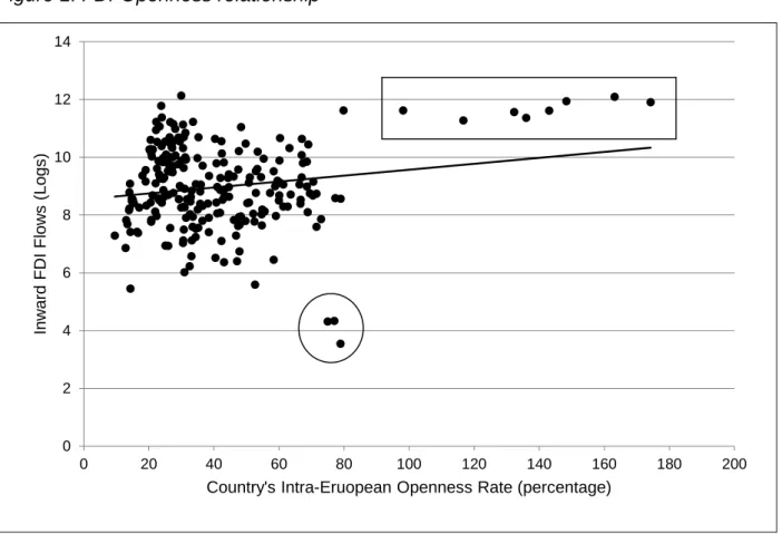
On a priori grounds it is not clear to what extent the fluctuations in trade and FDI flows are interrelated. In this sense, Figure 1 displays a scatter plot of inward FDI flows (measured in natural logarithms) against the intra-European Openness rate. Each point accounts for the pair inward FDI–Openness rate for a country in a certain year. The Figure
suggests a positive correlation between both variables, but this is very reliant upon the inclusion of Belgium and Luxembourg in the Figure (points for Benelux are located inside the square at the upper right corner); moreover, it is easy to identify another group of outliers (inside the circle), corresponding in this case to Ireland in 1995, 1996 and 1997. The rest of dots do not appear to follow a definite pattern: the trend line would be horizontal if Benelux was removed from the sample. The connection between trade and FDI within Europe, thus, is not straightforward.
Figure 1. FDI-Openness relationship
Source: Own elaboration.
Data used in this study come mainly from the OECD. The International Direct Investment database provides data on bilateral foreign direct investment. FDI data is documented on an aggregate basis and measured in current US dollars. Data on bilateral exports, disaggregated by industries, are computed by the OECD in its Structural Analysis database (STAN). The GDPs in real terms and US dollars are taken from the OECD National Accounts Dataset. The FDI and Exports series have been deflated using the GDPs deflators included in the National Accounts Dataset. Data provided by the Centre
d´Etudes Prospectives et d´Informations Internationals (CEPII) is employed to account
for other variables included in our analysis, such as adjacency, common language and 0 2 4 6 8 10 12 14 0 20 40 60 80 100 120 140 160 180 200 Inw ar d F D I F low s ( Logs )
Country's Intra-Eruopean Openness Rate (percentage)
bilateral distances. Bilateral geodesic distances are calculated following the great circle formula, which uses latitudes and longitudes of the most important cities/agglomerations (in terms of population) in each country.
Relative Factor Endowments ratios (RFE) have been constructed using data on skilled7
and total employment from the Yearbook of Labour Statistics published by the International Labour Organization (ILO). Finally, the Corruption Perception Index elaborated by Transparency International is included in the specifications as an institutional control variable. This index ranks from 0 (high perception of corruption) to 10 (low corruption).
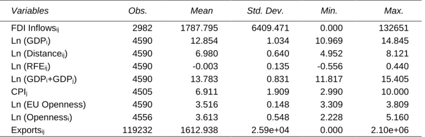
Table 2 presents the descriptive statistics of the main variables used in the study.
Table 2. Descriptive Statistics
Variables Obs. Mean Std. Dev. Min. Max.
FDI Inflowsij 2982 1787.795 6409.471 0.000 132651 Ln (GDPi) 4590 12.854 1.034 10.969 14.845 Ln (Distanceij) 4590 6.980 0.640 4.952 8.121 Ln (RFEij) 4590 -0.003 0.135 -0.556 0.440 Ln (GDPi+GDPj) 4590 13.783 0.831 11.817 15.405 CPIj 4505 6.911 1.909 2.990 10.000 Ln (EU Openness) 4590 3.516 0.148 3.309 3.809 Ln (Opennessi) 4556 3.613 0.548 2.228 5.160
Exportsij 119232 1612.938 2.59e+04 0.000 2.10e+06
Source: Own elaboration.
Notes: All variables in real terms. Bilateral FDI inflows and Exports are in levels (millions 2005US$).
4. Home bias estimation and empirical specification for FDI.
As stated above, the objectives of the paper are to investigate the sign of the relationship between trade and FDI flows within the EU by using the evolution of the home bias as an alternative measure of commercial integration, and to analyse the FDI pattern for the countries in our sample. Next, we shall present the results obtained when estimating the home bias and afterwards we shall describe the analysis pursued in order to understand the FDI pattern within the EU, employing as one of the key variables precisely the home bias computed before.
7 Skilled employment is defined as the sum of occupational categories 1 (legislators, senior officials and managers), 2
(professionals) and 3 (technicians and associate professionals) from the ISCO-88 classification. 8
4.1. Estimation of the Home Bias for the European Union (EU-19).
Different variables, such as the openness rate or the evolution in tariffs, have been used by the literature to measure commercial integration. Some contributions suggest that the performance of the home bias can be used as a measure of trade openness (Balta and Delgado, 2009). We have chosen to employ this last indicator since it may capture other dimensions (informal barriers, preferences) that ultimately determine commercial integration, and which are not included in alternative measures. In effect, the home bias measures the difference between the external and the internal (i.e. domestically oriented) trade of each country, thus capturing all factors which affect consumers’ decisions in favor of domestic good and services as opposed to those produced in other countries.
The home bias has received a remarkable deal of attention in the literature. The path breaking contribution of McCallum (1995), which used a gravity model as his framework of analysis and found a substantial degree of home bias in the Canadian-USA trade, was followed by other pieces of research covering OCDE countries (Wei, 1996), the EU (Nitsch, 2000; Chen, 2004; Qian, 2007; Martinez et al. 2012b) and regions (Combes et al., 2005; Wolf, 2009; Llano et al., 20011).
In its simplest form (Tinbergen, 1962), the gravity equation states that the volume of trade between any two countries is positively correlated with the economic size of the exporter and importer countries and negatively associated with the distance between them. Further extensions have introduced natural or artificial trade resistances (Anderson, 1979; Bergstrand, 1985; Anderson and Van Wincoop, 2003).
According to Anderson and Van Wincoop (2003), the gravity equation for trade is specified as follows: 𝑥𝑥𝑖𝑖𝑖𝑖𝑖𝑖 = 𝑦𝑦𝑖𝑖𝑖𝑖𝑦𝑦𝑦𝑦𝑗𝑗𝑖𝑖 𝑖𝑖𝑤𝑤 � 𝑖𝑖𝑖𝑖𝑗𝑗 𝑃𝑃𝑖𝑖𝑖𝑖𝑃𝑃𝑗𝑗𝑖𝑖� 1−𝜎𝜎 (1)
where xij measures exports from the exporter i country to the importer j country in year t.
yit and yjt are the gross domestic product of the exporter and importer countries. ytw is the
world GDP. tij stands for the bilateral trade barrier between country i and country j. Price
indices Pit and Pjt are, in the terminology of Anderson and Van Wincoop (2003),
“multilateral resistance” variables since they depend on all bilateral barriers or resistances (tij).
Thus, the gravity equation for trade to be estimated is as follows:
𝑥𝑥𝑖𝑖𝑖𝑖𝑖𝑖𝑖𝑖 = 𝛽𝛽0+ 𝛽𝛽1𝑙𝑙𝑙𝑙(𝑦𝑦𝑖𝑖𝑖𝑖) + 𝛽𝛽2𝑙𝑙𝑙𝑙�𝑦𝑦𝑖𝑖𝑖𝑖� + 𝛽𝛽3𝑙𝑙𝑙𝑙�𝐷𝐷𝐷𝐷𝐷𝐷𝐷𝐷𝑖𝑖𝑖𝑖� + 𝛽𝛽4�𝐷𝐷𝑖𝑖𝑖𝑖� +
+ 𝛽𝛽5(𝐻𝐻𝐻𝐻𝐻𝐻𝐻𝐻𝑖𝑖) + 𝜂𝜂𝑖𝑖+ 𝜂𝜂𝑖𝑖+ 𝜂𝜂𝑖𝑖+ 𝜂𝜂𝑖𝑖+ 𝜀𝜀𝑖𝑖𝑖𝑖𝑖𝑖𝑖𝑖 (2)
where: Xijkt are the k-sector bilateral exports from country i to country j in year t. yit and yjt
are the GDPs of countries i and j, respectively. Distij stands for the bilateral trade barrier
between country i and country j (the bilateral distance) and Dij captures different
characteristics of the exporter and importer countries such as sharing a common
language or land border, being an island or being landlocked. Homet is a dummy variable
which takes value 1 for intra-national trade and 0 otherwise. Additionally, the model
includes origin and destination (ηi, ηj) as well as industry and time (ηk, ηt) fixed effects in
order to account for the unobserved price indices or “multilateral resistance” mentioned
by Anderson and Van Wincoop (2003)8. ε
ijkt refers to the error term.
We have estimated the border effect by means of a gravity equation employing data on
bilateral trade for 23 sectors of activity9 among 19 European countries10 over the period
1995 to 2009. We employ a Poisson Pseudo-Maximum Likelihood model (PPML), proposed by Santos-Silva and Tenreyro (2006), in order to overcome the disadvantages of a log-linear specification of the gravity model. These authors showed that, in the presence of heteroskedasticity in the error term, the parameters of log-linearized models estimated by OLS lead to biased estimations of the true elasticities. In addition, log-linearization is incompatible with the existence of zeros in the dependent variable. The PPML method estimates the parameters by entering the dependent variable in levels while the independent ones are expressed in natural logarithms, thus providing a natural
way to deal with zeros in the data11.
On an a priori basis, bilateral exports from country i to country j are supposed to show a positive correlation with the economic sizes of both countries. Sharing special characteristics such as language or a common land border reduce transaction costs and
8 Since the multilateral resistance terms are not observable, it is a common practice to use importer and exporter fixed
effects to replace them; this approach, according to Feenstra (2002), provides consistent estimates and is easy to implement.
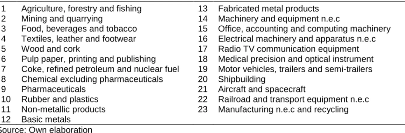
9 See table A1 in the appendix.
10 Austria, Benelux (Belgium-Luxembourg), Czech Republic, Denmark, Finland, France, Germany, Greece, Hungary,
Ireland, Italy, Netherlands, Poland, Portugal, Slovakia, Spain, Sweden, and United Kingdom.
11 Panel dataset has 111,780 potential observations (23-sectors x 18-exporting countries x 18-importing countries x
15-years) of which 4,463 are zero.
10
consequently foster bilateral trade. The bilateral distance between countries i and j should act as a barrier to trade and hence exhibit a negative sign.
For the purpose of this paper, the key parameters in equation (2) are those corresponding
to the dummy for Homet since we can recover yearly border effects from their point
estimates. The exponential of the coefficient of Homet, is the ratio of intra-national trade
to international trade for a certain year, country or industry, after controlling for the size of
GDP, distance, language, adjacency and others12 . Therefore, small point estimates for
the home dummies indicate a low relative weight of intra-national trade and thus a large relevance of international trade for the correspondent countries, industries or years of the sample, and substantial trade integration (Qian, 2007; Balta and Delgado, 2009; Martinez et al, 2012b). If border effects diminish over time, it means that intra-national trade becomes less important relative to international trade and hence preference for domestically produced goods, as opposed to foreign ones, declines over the period considered, other things equal.
We have estimated two types of Home Bias (HB). First, we compute the HB for the entire EU-19 sample over the years 1995-2009 in order to capture the size of the EU commercial integration as a whole. Second, we compute the HB for each country to help understand how individual HBs affect bilateral flows of FDI among EU countries. Table A2 in appendix reports the original estimations using different specifications of the gravity equation (2). As shown in Table A2, in all specifications, the basic gravity explanatory variables are highly significant and the coefficients have the expected signs. In order to compute the border effect from the estimations we take the exponential of the point estimate of the
home variable13.
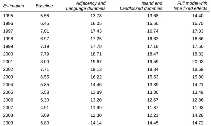
Table 3 summarizes the evolution of the border effects obtained from the estimations reported in the appendix and for different model specifications.
12 See, among others, McCallum (1995), Helliwell (1996), Wei (1996), Nitsch (2000), Wolf (2009), Chen (2004) and Liu
et al. (2010) for further explanation.
13 For example, to calculate the HB for 2009, we use the estimation at the fourth column and year 2009
(Home2009=2.689); this figure means that, on average, a European country traded 14.7 times (exp2.689=14.71) more
with itself than with another European partner.
11
Table 3. Evolution of the home bias
Estimation Baseline Adjacency and Language dummies
Island and Landlocked dummies
Full model with time fixed effects
1995 5.58 13.78 13.68 14.40 1996 6.45 16.05 15.50 15.75 1997 7.01 17.43 16.74 17.03 1998 6.97 17.25 16.63 16.86 1999 7.19 17.78 17.18 17.50 2000 7.79 18.71 18.47 18.82 2001 8.00 19.67 19.59 20.03 2002 7.71 19.13 18.34 18.69 2003 6.55 16.22 15.53 15.80 2004 5.85 14.45 13.89 14.21 2005 5.58 13.89 13.30 13.49 2006 5.30 13.20 12.67 12.86 2007 4.91 11.99 11.87 11.93 2008 5.09 12.30 12.21 14.28 2009 5.80 14.14 14.45 14.72
Source: Own elaboration.
Notes: Estimated Border Effects are calculated as the exponential of the β-estimates for the Home variables in table A2 (expHome
t). Columns are presented in the same order as in table A2.
The first column exhibits the results from the standard gravity equation where the economic size of the exporter and importer countries and the distance between them are considered. Calculations reported in Column 2 include dummy variables for adjacency and language. The last two columns display results from equations that include other potentially important features for trade, as being an island or landlocked, either for the
exporter and importer countries14. The average overall border effect shows a net increase
of around 3% from 1995 to 2009 for the EU-19 countries. Point estimates for the border effects in column 1 show lower values than in the rest of columns; however, since this is a very simple model where some likely relevant variables are omitted, those coefficients may be biased. Once dummy variables are included and different fixed effects are considered, the border effects rise but display comparable values across specifications. A very similar pattern over time arises for the border effect estimates in all the specifications, suggesting three sub-periods. In the first one, 1995-2001, the values of the HB grow over time around 40%. A second sub-period, from 2002 to 2007, is characterised by a sharp decline in border effects, also close to 40%; finally, the border
14 See Martinez et al. (2012b) for further discussion on the coefficients and their interpretation.
12
effect mounts again in the last two years of analysis, between 18% and 23%, this increase being especially important in 2009 when the border effect augments between 14% and 19% from the previous year, depending on the specification considered. These results fit remarkably well the picture which arises from the descriptive analysis of the data.
We have also computed the evolution of the border effect from a country point of view by estimating the country-specific evolution of the home bias over the period considered.
Estimated border effects and intra-European openness rate15 for each country are
presented in Figure 2.
The results offer a different picture depending on the country but we can also observe common trends. In general terms, a clear decrease of the border effect in 15 out of the 19 countries considered can be seen. When sub-periods are analyzed, twelve economies show an increase of the home bias until 2001-2002, followed by a sharp fall afterwards. Similarly, estimates show a rise of the border effect, for all countries, in 2009.
The analysis by individual countries suggests that the Central and Eastern European economies (Poland, Czech Republic, Hungary and Slovakia) exhibit the highest values for the border effect, with Hungary ranking on the first position; these figures indicate, in turn, that exports from these countries to the rest of countries in the sample in 1995 were small relative to the domestic demand. The decline of the HB over time is remarkable, and can be traced back to the process of EU enlargement and the subsequent possibilities of accession to a larger market. Estimates for Slovakia and Poland at the end of the period, for example, are comparable to those of France, Italy or Spain.
Benelux and the Netherlands exhibit the lowest levels of the home bias. Moreover, the border effect in these countries has decreased significantly along the period. Germany and the UK also display a large level of trade integration compared to the rest of the EU-19. Some of the peripheral countries, such as Finland, Ireland, Greece and Portugal, make up another group of similar characteristics, with similar levels of the HB and with an evolution over time which ends up in a slightly higher border effect at the end of the period with respect to 1995. The remaining countries in the sample (Austria, Denmark, France, Italy, Spain and Sweden) show a clear downward trend in the HB, with Sweden and Denmark displaying higher home bias values within the sub-group. The openness rate shows a behavior which is almost perfectly the inverse of the home bias.
15 Intra-European Openness Rate is computed as exports plus imports to/from the rest of the EU-19 divided by GDP.
13
Figure 2. Country specific home bias and intra-European openness rate
Austria Belgium-Luxembourg Czech Republic Denmark Finland
France Germany Greece Hungary Ireland
Italy Netherlands Poland Portugal Slovakia
Spain Sweden United Kingdom
Source: own elaboration
Notes: Solid lines account for the estimated border effect while the dotted ones represent the country’s intra-European Openness Rate. Left vertical axes are the reference for the openness rate (in percentage). Right vertical axes are the scale for the border effect. Data on exports, imports and GDP are from the OECD. Border Effects have been estimated by means of the gravity equation (2).
4.2. Gravity model for FDI.
In this subsection we present the empirical specification employed to ascertain which kind of model reflects better the behaviour of FDI flows within EU-19. To discriminate among the different FDI models, the theoretical literature establishes that the main determinants underlying location choices can be summarized in the following: size and market potential in the home and host countries, the difference in resource endowments between the home and host countries, and the distance between both countries. In turn, the potential of the host market may be contingent on aspects such as the degree of macroeconomic stability and the quality of institutions. These ideas can be easily accommodated within the framework proposed by Kleinert and Toubal (2010); these authors design a FDI gravity model which allows to include additional variables such as the trade protection indexes (see Carr et al, 2001; and Braconier et al, 2005; as well). This paper employs this basic setup, but proposes a novel approach to build the trade indicators from the estimation of the home bias or border effect.
Some papers have shown that the rationale behind the gravity equation for trade can also be employed to model the determinants of FDI (Eaton and Tamura, 1996; Graham, 1996; Brenton et al, 1999). Empirical studies that adapted the gravity equation for trade to FDI can be found, among others, in Brainard (1997), Markusen and Maskus (2002) and Bergstrand and Egger (2007). More in particular, Kleinert and Toubal (2010) provide the theoretical foundations for the application of the gravity equation to foreign affiliates’
sales16. This theoretical approach serves as a benchmark to develop a gravity equation
that could be modified to test for horizontal and vertical FDI models. For the proximity-concentration model –horizontal– the theoretical specification will be as follows:
𝑓𝑓𝑓𝑓𝐷𝐷𝑖𝑖𝑖𝑖𝑖𝑖 = 𝑦𝑦𝑖𝑖𝑖𝑖�𝜏𝜏𝐷𝐷𝑖𝑖𝑖𝑖𝜂𝜂1�
(1−𝜎𝜎)(1−𝜀𝜀)
𝑦𝑦𝑖𝑖𝑖𝑖 (3)
where fdiijt measures the aggregate FDI flows from country i to country j in year t. yit is the
home country GDP in real terms, which proxies for its supply capacity, and yjt is the host
country GDP in real terms, which accounts for its market potential. Distance costs, 𝜏𝜏𝐷𝐷𝑖𝑖𝑖𝑖𝜂𝜂1,
are an increasing function of geographical distance between i and j with 𝜏𝜏 being unit
distance costs of the iceberg type and η1>0.
16 Although this specification of the gravity model is intended to analyse sales of foreign affiliates, it also may be used
to account for FDI (See Bergstrand and Egger, 2007). 15
The vertical model for FDI flows can be characterized as:
𝑓𝑓𝑓𝑓𝐷𝐷𝑖𝑖𝑖𝑖𝑖𝑖 = 𝛿𝛿(1 − 𝜇𝜇)�𝑦𝑦𝑖𝑖𝑖𝑖+ 𝑦𝑦𝑖𝑖𝑖𝑖�𝑔𝑔2�𝑦𝑦𝑖𝑖𝑖𝑖⁄ �𝑓𝑓�𝜏𝜏𝑦𝑦𝑖𝑖𝑖𝑖 𝑖𝑖𝑖𝑖𝑍𝑍�𝑔𝑔1�𝑆𝑆𝐿𝐿𝑖𝑖𝑖𝑖⁄�𝑆𝑆𝑖𝑖𝑖𝑖+𝑆𝑆𝑗𝑗𝑖𝑖�
𝑖𝑖𝑖𝑖⁄�𝐿𝐿𝑖𝑖𝑖𝑖+𝐿𝐿𝑗𝑗𝑖𝑖�� (4)
Where fdiijt measures again the aggregate FDI flows from country i to country j in year t.
𝑔𝑔2�𝑦𝑦𝑖𝑖𝑖𝑖⁄ � is a function of the income ratio, 𝜏𝜏𝑦𝑦𝑖𝑖𝑖𝑖 𝑖𝑖𝑖𝑖𝑍𝑍 is a function of the distance costs, and
𝑔𝑔1�𝑆𝑆𝐿𝐿𝑖𝑖𝑖𝑖𝑖𝑖𝑖𝑖⁄⁄�𝐿𝐿�𝑆𝑆𝑖𝑖𝑖𝑖𝑖𝑖𝑖𝑖+𝑆𝑆+𝐿𝐿𝑗𝑗𝑖𝑖𝑗𝑗𝑖𝑖��� is a function of the relative factor endowment ratio between country i and
country j. The labor shares are computed as the proportion of the home country skilled
labor in total skilled labor of the two countries,𝑆𝑆𝑖𝑖⁄�𝑆𝑆𝑖𝑖 + 𝑆𝑆𝑖𝑖�, and the share of the home
country unskilled labor, 𝐿𝐿𝑖𝑖⁄�𝐿𝐿𝑖𝑖 + 𝐿𝐿𝑖𝑖�.
Equations (3) and (4) provide the baseline specification and can be transformed into empirical models to be estimated as follows:
𝑓𝑓𝑓𝑓𝐷𝐷𝑖𝑖𝑖𝑖𝑖𝑖 = 𝛼𝛼 + 𝛽𝛽1ln(𝑦𝑦𝑖𝑖𝑖𝑖) + 𝛽𝛽2ln�𝑦𝑦𝑖𝑖𝑖𝑖� + 𝛽𝛽3ln�𝐷𝐷𝐷𝐷𝐷𝐷𝐷𝐷𝑖𝑖𝑖𝑖� + 𝛽𝛽4ln(𝐻𝐻𝐻𝐻𝐻𝐻𝐻𝐻 𝐵𝐵𝐷𝐷𝐵𝐵𝐷𝐷𝑖𝑖) +
+𝛽𝛽5𝐶𝐶𝐶𝐶𝐶𝐶𝑖𝑖𝑖𝑖+ 𝜂𝜂𝑖𝑖 + 𝜂𝜂𝑖𝑖+ 𝜂𝜂𝑖𝑖+ 𝜀𝜀𝑖𝑖𝑖𝑖𝑖𝑖 (5)
𝑓𝑓𝑓𝑓𝐷𝐷𝑖𝑖𝑖𝑖𝑖𝑖 = 𝛼𝛼 + 𝛽𝛽1ln(𝑦𝑦𝑖𝑖𝑖𝑖) + 𝛽𝛽2ln�𝑦𝑦𝑖𝑖𝑖𝑖� + 𝛽𝛽3ln�𝐷𝐷𝐷𝐷𝐷𝐷𝐷𝐷𝑖𝑖𝑖𝑖� + 𝛽𝛽4ln(𝐻𝐻𝐻𝐻𝐻𝐻𝐻𝐻 𝐵𝐵𝐷𝐷𝐵𝐵𝐷𝐷𝑖𝑖) +
+ 𝛽𝛽5ln�𝑦𝑦𝑖𝑖𝑖𝑖+ 𝑦𝑦𝑖𝑖𝑖𝑖� + 𝛽𝛽6𝑅𝑅𝑅𝑅𝑅𝑅𝑖𝑖𝑖𝑖𝑖𝑖+ 𝛽𝛽7𝐶𝐶𝐶𝐶𝐶𝐶𝑖𝑖𝑖𝑖+ 𝜂𝜂𝑖𝑖 + 𝜂𝜂𝑖𝑖+ 𝜂𝜂𝑖𝑖+ 𝜀𝜀𝑖𝑖𝑖𝑖𝑖𝑖 (6)
Equation (5) above corresponds to horizontal FDI models while equation (6) refers to
vertical schemes. fdiijt are the bilateral investment flows from country i to country j in year
t. yit and yjt are the GDPs of countries i and j, respectively. Distij stands for the bilateral
distance between home and host countries. The Home Biast is estimated by using a
gravity model, as detailed above; its evolution over time reflects the degree of trade
integration between the home and host country. RFEijt is the relative factor endowment
ratio, defined as 𝐿𝐿𝑙𝑙�𝑆𝑆𝑖𝑖𝑖𝑖⁄�𝑆𝑆𝑖𝑖𝑖𝑖+ 𝑆𝑆𝑖𝑖𝑖𝑖�� − 𝑙𝑙𝑙𝑙�𝐿𝐿𝑖𝑖𝑖𝑖⁄�𝐿𝐿𝑖𝑖𝑖𝑖+𝐿𝐿𝑖𝑖𝑖𝑖�� . CPIjt is the Corruption Perception Index from Transparency International and proxies for the degree of institutional
environment. Additionally, the model includes origin, destination, and time (ηi, ηj, ηt) fixed
effects. εijt refers to the error term.
With respect to the estimation methodology, we have used bilateral data from a panel of 19 European countries for the period 1995-2009. Following Santos-Silva and Tenreyro (2006) again, we have employed a Poisson Pseudo-Maximum Likelihood model (PPML).
5. Results.
This section discusses the results obtained when trying to capture the impact of intra-European trade integration on the bilateral FDI flows within the nineteen intra-European countries, using the gravity model specifications discussed above. Figure 3 shows the correlation between the Home Bias and FDI inflows. More specifically, FDI for a reporting country accounts for the logarithm of the aggregate flows from the rest of the European countries in the sample. The figure suggests a negative relationship between FDI and the Home Bias. Thus, we may expect negative coefficients in the estimation of the gravity model for FDI. As we did in Figure 1, we have also identified the Benelux (right upper corner square) and Ireland in 1995, 1996 and 1997 (circle). It is apparent that, when using the Home Bias as an index of trade, the connection between commercial integration and FDI within Europe (see Figure 3) appears clearer and more definite than when the openness rate is employed as in Figure 1.
Figure 3. FDI–Home Bias relationship
Source: Own elaboration. 0 2 4 6 8 10 12 14 0 1 2 3 4 5 6 7 8 9 10 Inw ar d F D I F low s ( Logs )
Home Bias (Logs)
Table 4 presents the estimation results from equations (5) and (6). The dependent variable is the real FDI inflows to country j from country i, being country j the reporting one.
The first two columns of Table 4 present the simplest horizontal and vertical FDI models. Point estimates regarding home and host GDPs display positive and significant values in both columns. The structural models in Kleinert and Toubal (2010) suggest that for the case of the horizontal model, the coefficients on both GDP variables should be equal to
one17. However, our results show that the restriction of both coefficients being equal to
unity is rejected at the 1% level (see column 1). Furthermore, according to Kleinert and Toubal, the structural vertical model predicts a negative value for the home country GDP estimate, which, as it can be observed, is not supported by our estimations either. Regarding column 2, the structural vertical model also suggests that the variable market
demand for goods (proxied by the sum of GDPs) should present an estimate equal to
unity and the relative factor endowment ratio (RFE) should be positive18. In these two
cases our empirical results present mixed evidence. While the sum of GDPs is negative and significant at the 10% level, the RFE ratio displays a positive and significant coefficient. In all cases, estimates regarding bilateral distance are in line with the theoretical models.
Estimations reported in columns 3 and 4 in Table 4 include the home bias, thus providing information on the trade–FDI relationship. In column 3, we include the home bias variable for the overall EU-19, while in column 4 we consider the investor and recipient home bias variables separately. In both cases results show a negative and highly significant coefficients for these variables, suggesting that the higher the home bias of a particular country, the lower the FDI inflows it attracts. This result points out to a complementary pattern between European commercial integration and FDI.
In order to test the robustness of these results columns 5 and 6 report the estimations when using the traditional openness variable. Whereas column 5 considers the intra-European openness rate, column 6 introduces the home and host country openness rates individually. Results from using these variables indicate, as in the previous cases, a complementary relationship between intra-European trade and FDI. Moreover, results show a similar pattern to those obtained using the home bias variable proposed in this paper.
17 See Kleinert and Toubal (2010) for further information.
18 The intuition is that the more skilled labour abundant is the home country relative to the host country, the larger the
bilateral FDI flows between them.
18
Another remarkable aspect that arises from the estimation is the impact of the economic crisis. In this sense, it is particularly interesting to test whether the FDI-Trade relationship has been affected by the financial and economic turbulences. We have addressed this issue by including an interaction term between the EU Home Bias and the time dummies for the years 2007, 2008 and 2009 (column 7) Results show an overall complementary relationship between EU Home Bias and FDI (see column 3 and 7) however, column 7 suggests that this complementary relationship has changed throughout the last years of the analysis. The coefficient for the interaction term in 2007 is negative and significant, whereas the point estimate for this variable in 2008 is not statistically significant; finally, it is positive and significant for 2009.
Results so far do not enable us to discriminate fully between horizontal and vertical strategies in the pattern of Intra-European FDI; hence, it seems to be a more complex and less straightforward phenomenon, perhaps a combination of a horizontal and a vertical model.
Table 4: Home Bias-FDI nexus by means of the gravity equation (1) (2) (3) (4) (5) (6) (7) ln (Yi) 0.715 *** 1.086 *** 1.093 *** 0.852 *** 1.093 *** 1.396 *** 1.093 *** (0.094) (0.179) (0.191) (0.188) (0.191) (0.178) (0.191) ln (Yj) 0.560 *** 0.880 *** 0.796 *** 0.620 *** 0.796 *** 1.259 *** 0.796 *** (0.086) (0.202) (0.222) (0.226) (0.222) (0.156) (0.222) ln (Distij) -1.358 *** -1.347 *** -1.189 *** -0.804 *** -1.189 *** -0.631 *** -1.189 *** (0.150) (0.137) (0.102) (0.111) (0.102) (0.115) (0.102) ln (Yi+Yj) -0.722 * -0.810 ** 0.748 ** -0.810 ** -1.010 *** -0.810 ** (0.371) (0.378) (0.361) (0.380) (0.327) (0.378) RFEij 2.323 *** 1.123 0.506 1.123 1.300 * 1.123 (0.752) (0.825) (0.635) (0.825) (0.760) (0.825) CPIj 0.296 *** 0.248 *** 0.296 *** 0.269 *** 0.296 *** (0.066) (0.069) (0.066) (0.058) (0.066) IRELANDj 0.765 ** 0.551 * 0.765 ** 0.855 *** 0.765 ** (0.381) (0.298) (0.381) (0.244) (0.381) CEEj -1.288 *** -0.479 ** -1.288 *** -0.694 *** -1.288 *** (0.193) (0.218) (0.193) (0.163) (0.193) EU HB -3.359 *** -1.336 *** (1.013) (0.164) Home Biasi -0.373 *** (0.079) Home Biasj -0.298 *** (0.103) EU OPEN 2.474 *** (0.746) OPENi 0.712 *** (0.226) OPENj 1.042 *** (0.266) EU HB * 2007 -0.263 ** (0.114) EU HB * 2008 -0.121 (0.082) EU HB * 2009 0.562 *** (0.069) Observations 2982 2982 2952 2952 2952 2952 2952 Test ln(Yi)=ln(Yj)=1 57.64 *** 1.45 2.74 2.96 2.74 4.97 * 2.74 p-value 0.000 0.483 0.254 0.227 0.254 0.083 0.254 Source: Own elaboration.
Notes: The dependent variable is the real bilateral FDI inflows to country 𝑗𝑗 from country 𝐷𝐷 (country j reporting country). Poisson pseudo-maximum likelihood estimation. Clustered robust standard errors in parenthesis. *, **, *** denote significantly different from 0 at 10%, 5% and 1% levels, respectively. Home country, host country and time fixed effects are included in all the regressions.
The next columns (3 to 7) show the results from estimations which include additional variables to test for the extended vertical model. The Corruption Perception Index (CPI) of the host country is included in order to control for a safe investment environment. Dummy variables for Ireland and the Central and Eastern European countries (CEE) as recipients of FDI are included. The rationale behind the introduction of these dummy variables deal with the fact that Ireland has reduced its corporation tax from 28.5% in 1999 to 12.5% in 2003 and afterwards, making the investment activity in that country
more profitable. In the case of the CEE countries, their particular idiosyncrasies and their relatively recent inclusion in the European Union may be relevant to attract FDI. Finally, commercial integration variables are considered to test the trade-FDI nexus.
Once the model is augmented, the lack of conclusiveness remains, as shown in columns 3 to 7. On the one hand, the sign and size of the home GDP and the goods market demand (sum of GDPs) do not match the predictions of the vertical theory. It is true that the coefficient for RFE displays the correct sign, positive, but the evidence in favour of the factor–proportion differentials argument is not robust enough, as the results are not statistically different from zero in all specifications -except for column 2-. On the other hand, although estimates for the home and host GDPs variable reject the hypothesis of unity in the horizontal model (column 1), the results emerging from the rest of the estimations cannot reject this hypothesis. As mentioned above, our results do not enable us to discriminate between horizontal and vertical models. Our results are in line with Braconier et al (2005) who find strong support for the knowledge capital hybrid model using data on foreign affiliate’s sales for 56 home and 85 host countries for 1986, 1990,
1994 and 199819.
CPI estimates show positive and significant values in all the specifications. Additionally point estimates across the specifications are very stable, ranging from 0.218 to 0.296. These results suggest the importance of having a corruption free environment when it comes to attract FDI flows. The dummy variable for Ireland is positive and significant, which might be due to the effect of a reduced corporate tax, ceteris paribus. Point estimates range from 0.551 to 1.119 and are significantly different from zero at the 5% and 1% levels.
Instead, dummies for CEE countries are negative. This suggests that there are still some factors, such as the insufficient development of the institutional framework and the rule of law, the uncertainty regarding property rights and the lack of a developed financial sector, which jeopardize FDI inflows. Finally, given the special characteristics of the Benelux and Ireland highlighted previously (see Figure 1), we have estimated the FDI models without these two countries, Table A3 in the appendix shows the outcome. Results obtained are similar and in line to those computed for the whole sample.
19 Kleinert and Toubal (2010) however, suggest the prevalence of the horizontal model when analysing foreign affiliates’
sales using the same data than Braconier et al (2005). 21
6. Conclusions.
The empirical analysis carried out and described in this paper states that commercial integration and FDI within the European Union display a relationship of complementarity. The novelty of our analysis is that this relationship is captured using the evolution of the home bias as the proxy for commercial integration. Results obtained regarding this variable, nonetheless, are indeed confirmed and reinforced when using more traditional indicators such as the openness rate. An interesting feature suggested by our empirical exercise is that this complementary relationship does not seem to carry over in the crisis years 2008 and 2009. Does it mean that this relationship has experienced a structural change or it is just a consequence of the dynamics propitiated by the crisis? This issue deserves further research, to be pursued in the next future.
The results also point out that the FDI pattern within the European Union cannot be classified according to clear cut vertical or horizontal models. Instead, it seems that FDI flows follows a combination of both and therefore a hybrid model. While factor proportions appear not to be as relevant as the possibility of gaining market share –thus pointing to a horizontal model–, the complementarity relation between commercial integration and FDI suggest some kind of vertical motivations.
Our findings support the idea that policies targeted to promote further consolidations of the European Single Market –removing informal trade barriers, enhancing market liberalization and reducing bureaucracy–, may have positive effects, not only regarding the commercial performance of the EU but also helping to intensify FDI flows among the European countries, and indirectly, stimulating economic growth.
References.
Alguacil, M., Cuadros, A., Orts, V., 2008. EU Enlargement and Inward FDI. Review of
Development Economics 12, 594-604.
Anderson, J., 1979. A Theoretical Foundation of the Gravity Equation. American
Economic Review 69, 106-116.
Anderson, J., Van Wincoop, E., 2003. Gravity with gravitas: a solution to the border puzzle. American Economic Review 93, 170-192.
Balasubramanian, V., Sapsford, D., Griffiths, D., 2002. Regional Integration Agreements and Foreign Direct Investment: Theory and Preliminary Evidence. The Manchester
School 70, 460-482.
Balta, N., Delgado, J., 2009. Home Bias and Market Integration in the EU. CESifo
Economic Studies 55, 110-144.
Bevan, A., Estrin, S., 2004. The determinants of foreign direct investment into European transition economies. Journal of Comparative Economics 32, 775-787.
Bergstrand, J., 1985. The Gravity Equation in International Trade: some Microeconomic Foundations and Empirical Evidence. Review of Economics and Statistics 67, 474-481.
Bergstrand, J., 1989. The Generalized Gravity Equation, Monopolistic Competition, and the Factor-Proportion Theory in International Trade. The Review of Economics and
Statistics 714, 143-153.
Bergstrand, J., Egger, P., 2007. A Knowledge-and-Physical-Capital Model of International Trade Flows, Foreign Direct Investment, and Multinational Enterprises. Journal of
International Economics 73, 278-308.
Blonigen, B., 2001. In Search of Substitution between Foreign Production and Exports.
Journal of International Economics 53, 81-104.
Blonigen, B., 2005. A Review of the Empirical Literature on FDI Determinants. Atlantic
Economic Journal 33, 383-403.
Braconier, H., Nörback, P.J., Urban, D., 2005. Reconciling the Evidence on the Knowledge-capital Model. Review of International Economics 13, 770-786.
Brainard, S., 1997. An Empirical Assessment of the Proximity-Concentration Trade-off between Multinational Sales and Trade. American Economic Review 87, 520-544. Brenton, P., Di Mauro, F., Lucke, M., 1999. Economic Integration and FDI: an Empirical Analysis of Foreign Investment in the EU and in Central and Eastern Europe.
Empirica 26, 95-121.
Buckley, P., Casson, M., 1976. The Future of the Multinational Enterprise. Holmes & Meier Publishers. New York.
Carr, D., Markusen, J., Maskus, K., 2001. Estimating the Knowledge-capital Model of the Multinational Enterprise. American Economic Review 91, 693-708.
Carstensen, K., Toubal, F., 2004. Foreign Direct Investment in Central and Eastern European countries: a dynamic panel analysis. Journal of Comparative Economics 32, 3-22.
Caves, R., 1971. International Corporations: The Industrial Economics of Foreign Investments. Economica 39, 1-27.
Chen, N., 2004. Intra-national versus international trade in the European Union: why do national borders matter. Journal of International Economics 63, 93-118.
Combes, P., Lafourcade, M., Mayer, M., 2005. The Trade-creating Effects of Business and Social. Journal of International Economics 63, 93-118.
Dunning, J., 1973. The Determinants of International Production. Oxford Economic
Papers 25, 289-336.
Eaton, J., Tamura, A., 1996. Japanese and US Exports and Investment as Conduits of Growth. NBER Working Paper No. 5457.
Egger, P., Pfaffermayer, M., 2004a. Foreign Direct Investment and European Integration in the 1990s. World Economy 27, 99-110.
Egger, P., Pfaffermayer, M., 2004b. Distance, Trade and FDI: A Hausman-Taylor SUR Approach. Journal of Applied Econometrics 19, 227-246.
Feenstra, R., 2002. Border effects and the gravity equation: consistent method for estimation. Scottish Journal of Political Economy 49, 491-506.
Fillat-Castejón, C., Francois, J., Wörz, J., 2008. Cross-Border Trade and FDI in Services.
CEPR Discussion Paper No. 7074.
Goldberg, L., Klein, M., 1999. International Trade and Factor Mobility: an Empirical Investigation. NBER Working Paper No. 7196.
Graham, E., 1996. On the Relationship among Foreign Direct Investment and International Trade in the Manufacturing Sector: Empirical Results for the United States and Japan. WTO Staff Working Paper RD-96-008.
Head, K., Mayer, T., 2004. The empirics of agglomeration and trade, in: Henderson, J.V., Thisse, J.F. (Eds.), Handbook of Regional and Urban Economics, Vol. 4. North-Holland, Amsterdam, pp. 2609-2669.
Head, K., Ries, J., 2001. Increasing returns versus national product differentiation as an explanation for the pattern of US-Canada trade. American Economic Review 91, 858-876.
Helliwell, J. F., 1996. Do national borders matter for Québec’s trade? Canadian Journal
of Economics 29, 507-522.
Helpman, E., 1984. A simple theory of trade with multinational corporations. Journal of
Political Economy 92, 451-471.
Helpman, E., Krugman, P., 1985. Market Structure and Foreign Trade. MIT Press. Cambridge, MA.
Helpman, E., Melitz, M., Yeaple, S., 2004. Export versus FDI with Heterogeneous Firms.
American Economic Review 94, 300-316.
Hymer, S., 1976. The International Operations of National Firms: a Study of Foreign
Direct Investment. MIT Press. Cambridge, MA.
Kleinert, J., Toubal, F., 2010. Gravity for FDI. Review of International Economics 18, 1-13.
Liu, X., Whalley, J., Xin, X., 2010. Non-tradable goods and the border effect puzzle.
Economic Modelling 27, 909-914.
Llano, C., Minondon, A., Requena, F., 2011. Is the Border Effect an Artefact of Geographical Aggregation? The World Economy 34, 1771-1778.
Martinez, V., Bengoa, M., Sanchez-Robles, B., 2012a. Foreign Direct Investment and Trade: Complements or Substitutes? Empirical Evidence for the European Union.
Technology and Investment 3, 105-112.
Martinez, V., Bengoa, M., Sanchez-Robles, B., 2012b. European Union and Trade Integration: Does the Home Bias Puzzle Matter? Revista de Economia Mundial 32, 173-188.
Markusen, J., Venables, A., 1998. Multinational Firms and the New Trade Theory. Journal
of International Economics 46, 183-203.
Markusem, J., Maskus, K., 2002. Discriminating among Alternative Theories of the Multinational Enterprise. Review of International Economic, 10, 694-707.
McCallum, J., 1995. National borders matter: Canada-US regional trade patterns.
American Economic Review 37, 615-623.
Mundell, R., 1957. International Trade and Factor Mobility. American Economic Review 57, 321-335.
Neary, J., 2009. Trade Costs and Foreign Direct Investment. International Review of
Economics and Finance 19, 207-218.
Nitsch, V., 2000. National borders and international trade: evidence from the European Union. Canadian Journal of Economics 33, 1091-1105.
Obstfeld, M., Rogoff, K., 2001. The six major puzzles in international macroeconomics: is there a common cause? in: Bernanke, B., Rogoff, K. (Eds.), NBER Macroeconomic
Annual 2000. MIT Press. Cambridge, MA, pp. 339-390.
Pfaffermayer, M., 1996. Foreign Outward Direct Investment and Exports I Austrian Manufacturing: Substitues or Complements? Weltwirtschaftliches Archiv 132,501-552.
Qian, Z., 2007. FDI and European Economic Integration, Master dissertation, M. A. Economics of International Trade and European Integration. MIMEO, University of Antwerp, Belgium.
Santos-Silva, J., Tenreyro, S., 2006. The Log of Gravity. The Review of Economics and
Statistics 88, 641-658.
Swenson, D., 2004. Foreign Investment and the Mediation of Trade Flows. Review of
International Economics 12, 609-629.
Tinbergen, J., 1962. Shaping the World Economy: Suggestions for an International
Economic Policy. Twentieth Century Fund, New York.
Türkcan, K., 2007. Outward Foreign Direct Investment and Intermediate Goods Exports: Evidence from the USA. Economie Internationale 112, 51-71.
UNCTAD, 2010a, 2011a. Trade and Development Report. United Nations. New York and Geneve.
UNCTAD, 2010b, 2011b. World Investment Report. United Nations. New York and Geneve.
Wei, S., 1996. Intra-national versus international trade: how stubborn are nations in global integration. NBER Working Paper No. 5531.
Wolf, N., 2009. Was Germany Ever United? Evidence from Intra- and International Trade.
The Journal of Economic History 69, 846-881.
Appendix.
Table A1. Sectors of activity.
1 2 3 4 5 6 7 8 9 10 11 12
Agriculture, forestry and fishing Mining and quarrying
Food, beverages and tobacco Textiles, leather and footwear Wood and cork
Pulp paper, printing and publishing Coke, refined petroleum and nuclear fuel Chemical excluding pharmaceuticals Pharmaceuticals
Rubber and plastics Non-metallic products Basic metals 13 14 15 16 17 18 19 20 21 22 23
Fabricated metal products Machinery and equipment n.e.c
Office, accounting and computing machinery Electrical machinery and apparatus n.e.c Radio TV communication equipment Medical precision and optical instrument Motor vehicles, trailers and semi-trailers Shipbuilding
Aircraft and spacecraft
Railroad and transport equipment n.e.c Manufacturing n.e.c and recycling Source: Own elaboration
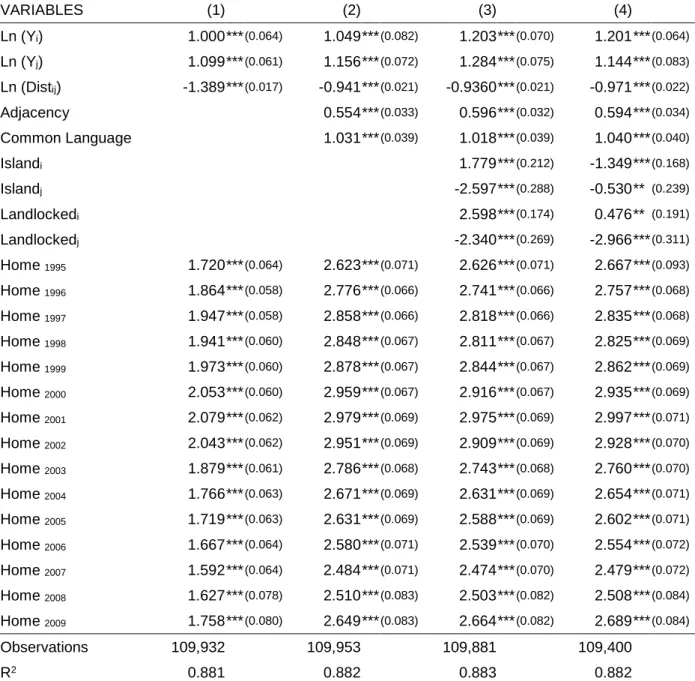
Table A2. Gravity equation for trade with yearly border effects VARIABLES (1) (2) (3) (4) Ln (Yi) 1.000 *** (0.064) 1.049 *** (0.082) 1.203 *** (0.070) 1.201 *** (0.064) Ln (Yj) 1.099 *** (0.061) 1.156 *** (0.072) 1.284 *** (0.075) 1.144 *** (0.083) Ln (Distij) -1.389 *** (0.017) -0.941 *** (0.021) -0.9360 *** (0.021) -0.971 *** (0.022) Adjacency 0.554 *** (0.033) 0.596 *** (0.032) 0.594 *** (0.034) Common Language 1.031 *** (0.039) 1.018 *** (0.039) 1.040 *** (0.040) Islandi 1.779 *** (0.212) -1.349 *** (0.168) Islandj -2.597 *** (0.288) -0.530 ** (0.239) Landlockedi 2.598 *** (0.174) 0.476 ** (0.191) Landlockedj -2.340 *** (0.269) -2.966 *** (0.311) Home 1995 1.720 *** (0.064) 2.623 *** (0.071) 2.626 *** (0.071) 2.667 *** (0.093) Home 1996 1.864 *** (0.058) 2.776 *** (0.066) 2.741 *** (0.066) 2.757 *** (0.068) Home 1997 1.947 *** (0.058) 2.858 *** (0.066) 2.818 *** (0.066) 2.835 *** (0.068) Home 1998 1.941 *** (0.060) 2.848 *** (0.067) 2.811 *** (0.067) 2.825 *** (0.069) Home 1999 1.973 *** (0.060) 2.878 *** (0.067) 2.844 *** (0.067) 2.862 *** (0.069) Home 2000 2.053 *** (0.060) 2.959 *** (0.067) 2.916 *** (0.067) 2.935 *** (0.069) Home 2001 2.079 *** (0.062) 2.979 *** (0.069) 2.975 *** (0.069) 2.997 *** (0.071) Home 2002 2.043 *** (0.062) 2.951 *** (0.069) 2.909 *** (0.069) 2.928 *** (0.070) Home 2003 1.879 *** (0.061) 2.786 *** (0.068) 2.743 *** (0.068) 2.760 *** (0.070) Home 2004 1.766 *** (0.063) 2.671 *** (0.069) 2.631 *** (0.069) 2.654 *** (0.071) Home 2005 1.719 *** (0.063) 2.631 *** (0.069) 2.588 *** (0.069) 2.602 *** (0.071) Home 2006 1.667 *** (0.064) 2.580 *** (0.071) 2.539 *** (0.070) 2.554 *** (0.072) Home 2007 1.592 *** (0.064) 2.484 *** (0.071) 2.474 *** (0.070) 2.479 *** (0.072) Home 2008 1.627 *** (0.078) 2.510 *** (0.083) 2.503 *** (0.082) 2.508 *** (0.084) Home 2009 1.758 *** (0.080) 2.649 *** (0.083) 2.664 *** (0.082) 2.689 *** (0.084) Observations 109,932 109,953 109,881 109,400 R2 0.881 0.882 0.883 0.882
Source: Own elaboration.
Notes: Poisson pseudo-maximum likelihood estimation. The dependent variable is the real bilateral exports from country i to country j. Clustered robust standard errors in parentheses. *, **, *** denote significant at the 10%, 5% and 1% level, respectively. Industry fixed effects and year-specific exporter and importer fixed effects are included in all the regressions (Feenstra, 2002). The last column also includes time fixed effects.
Table A3: Home Bias-FDI nexus (without Benelux and Ireland) (1) (2) (3) (4) (5) (6) (7) ln (Yi) 0.812 *** 1.357 *** 1.433 *** 1.250 *** 1.433 *** 1.546 *** 1.433 *** (0.083) (0.167) (0.158) (0.183) (0.158) (0.175) (0.158) ln (Yj) 0.772 *** 1.273 *** 1.222 *** 1.177 *** 1.222 *** 1.206 *** 1.222 *** (0.080) (0.145) (0.141) (0.143) (0.141) (0.146) (0.141) ln (Distij) -1.098 *** -1.087 *** -0.964 *** -0.885 *** -0.964 *** -0.914 *** -0.964 *** (0.168) (0.143) (0.138) (0.123) (0.138) (0.151) (0.138) ln (Yi+Yj) -1.153 *** -1.350 *** -1.448. *** -1.350 *** -1.400 *** -1.350 *** (0.329) (0.287) (0.292) (0.287) (0.283) (0.287) RFEij 2.737 *** 0.786 0.285 0.786 0.048 0.786 (0.841) (0.957) (0.732) (0.957) (0.968) (0.957) CPIj 0.344 *** 0.275 *** 0.344 *** 0.327 *** 0.344 *** (0.048) (0.054) (0.048) (0.055) (0.048) CEEj -0.761 *** -0.590 ** -0.761 *** -0.787 *** -0.761 *** (0.176) (0.212) (0.176) (0.184) (0.176) EU HB -2.427 ** -0.999 *** (1.209) (0.194) Home Biasi -0.289 *** (0.081) Home Biasj -0.078 (0.065) EU OPEN 1.788 ** (0.891) OPENi 0.469 ** (0.228) OPENj 0.164 (0.270) EU HB * 2007 -0.159 (0.131) EU HB * 2008 -0.102 (0.115) EU HB * 2009 0.415 *** (0.084) Observations 2321 2321 2292 2292 2292 2292 2292 Test ln(Yi)=ln(Yj)=1 13.28 *** 4.83 * 8.13 ** 1.99 8.13 ** 14.04 *** 8.13 ** p-value 0.001 0.090 0.017 0.370 0.017 0.001 0.017
Source: Own elaboration.
Notes: The dependent variable is the real bilateral FDI inflows to country 𝑗𝑗 from country 𝐷𝐷 (country j reporting country). Poisson pseudo-maximum likelihood estimation. Clustered robust standard errors in parenthesis. *, **, *** denote significantly different from 0 at 10%, 5% and 1% levels, respectively. Home country, host country and time fixed effects are included in all the regressions.