in Science and Engineering, CMMSE 2010 27–30 June 2010.
A Rakhmanov-like theorem for orthogonal polynomials on
Jordan arcs in the complex plane
C. Escribano1, M. A. Sastre1, A. Giraldo1 and E. Torrano1
1 Departamento de Matem´atica Aplicada, Facultad de Inform´atica, Universidad Polit´ecnica de Madrid
emails: cescribano@fi.upm.es,masastre@fi.upm.es,agiraldo@fi.upm.es, emilio@fi.upm.es
Abstract
Rakhmanov’s theorem establishes a result about the asymptotic behavior of the elements of the Jacobi matrix associated with a measureµwhich is defined on the intervalI= [−1,1] withµ0>0 almost everywhere onI. In this work we give a weak version of this theorem, for a measure with support on a connected finite union of Jordan arcs on the complex plane, in terms of the Hessenberg matrix, the natural generalization of the tridiagonal Jacobi matrix to the complex plane.
Key words: Hessenberg matrix, regular measures, Riemann map.
1
Introduction
In this paper, we consider regular Borel measuresµdefined on subsets of the complex plane which are Jordan arcs, or connected finite union of Jordan arcs, and we show how the support of µ is determined by the entries of the Hessenberg matrix D associated with µ. The Hessenberg matrix is the natural generalization of the tridiagonal Jacobi matrix to the complex plane and, in the particular case of measures with support the unit circleT, the Hessenberg matrix is a Toeplitz matrix.
Our result represents a broader, although weaker, extension of Rakhmanov’s theo-rem toC. In the real case, Rakhmanov’s theorem [15, 16] states that, if the support of a Borel measure is [−1,1] and µ0 >0 almost everywhere in [−1,1], then a
n → 12 and bn→0, wherean are the sequences of elements in the subdiagonal and superdiagonal,
andbn are the sequences of elements in the diagonal, in the Jacobi matrixJ associated
with µ. Moreover, if the support of µ is the interval [−2a+b, b+ 2a], then the above limits are, respectively,an→aybn→b. Conversely, if we know that µ0 >0 and that
of J we could obtain the support of µ, i.e., if an → a y bn → b then the support is [−2a+b, b+ 2a].
Generalizations of Rakhmanov’s theorem to orthogonal polynomials and to orthog-onal matrix polynomials on the unit circle has been given in [13] and [22]. The case of orthogonal polynomials in an arc of circumference has been studied in [2]).
There exist some previous results relating the properties of D and the support of µ. For example, if the Hessenberg matrix D defines a subnormal operator [12] in `2, then the closure of the convex hull of its numerical range agrees with the convex hull of its spectrum. On the other hand, the spectrum of the matrixDcontains the spectrum of its minimal normal extension N = men(D) which is precisely the support of the measure [6].
In this work we show that, in the case of regular measures µ whose support is a Jordan arc or a connected union of Jordan arcs in the complex planeC, the limits of the values at the diagonals of the Hessenberg matrixD of µ, supposing those limits exist, determine the terms of the coefficients of the series expansion of the Riemann mapφ(z) (see [20]) which applies conformally the exterior of the unit disk in the exterior of the support of the measure. As a consequence, the support of µ can be determined just knowing the limits of the values at the diagonals of its Hessenberg matrixD.
For general information on the theory of orthogonal polynomials, we recommend the books [4, 20] by T. S. Chihara and G. Szeg¨o, respectively, and the survey [11] by Golinskii and Totik.
2
Main result
Let µ(z) be a regular positive Borel measure with compact support Ω in the complex plane. Let P be the space of polynomials. The associated inner product is given by the expression
hQ(z), R(z)iµ=
Z
supp(µ)
Q(z)R(z)dµ(z),
for R, S ∈ P. Then there exists a unique orthonormal polynomials sequence (ONPS)
{Pn(z)}∞
n=0 associated to the measureµ (see [4], [8] or [20]).
In the space P2(µ), closure of the polynomials spaceP inL2µ(Ω), we consider the multiplication by z operator. Let D = (djk)∞j,k=0 be the infinite upper Hessenberg
matrix of this operator in the basis of ONPS {Pn(z)}∞
n=0, hence
zPn(z) = n+1 X
k=0
dk,nPk(z), n≥0, (1)
withP0(z) = 1 whenc00= 1.
It is a well known fact that the monic polynomials are the characteristic polynomials of the finite sections ofD.
A Jordan arc inCis any subset ofChomeomorphic to the closed interval [0,1] on the real line.
A measure µ is regular if lim
n→∞ 1 n
√
γn = cap(supp(µ)), the capacity of the support
of µ, where theγn are the conductor coefficients of the orthonormal polynomials, i.e., Pn(z) =γnzn+. . ..
An infinite matrixT = (ai,j)∞i,j=0 is a Toeplitz matrix if each descending diagonal
from left to right is constant, i.e, there exists (ai)i∈Z such that ai,j =ai−j, for every i, j∈N∪{0}. Given a Toeplitz matrixT, the Laurent series whose coefficients are the entriesai defines a function known as the symbol ofT.
We are now in a position to state and prove the main result of the paper.
Theorem 1. Let D = (dij)∞i,j=1 be a Hessenberg matrix associated with a measure µ with compact support on the complex plane. Assume that:
1. The measure µis regular with supportsupp(µ) a Jordan arc or a connected finite union of Jordan arcsΓ such that C\Γ is a simply connected set of the Riemann sphereC∞.
2. There exists a Hessenberg-Toeplitz matrix T such that D−T defines a compact operator in`2 with its rows in `1.
Then, the symbol of T is the Riemann function φ:C∞\D→C∞\Γ
Proof. Since supp(µ) = Γ is a compact set and C∞\Γ is connected, we can apply Merguelyan’s theorem [9, p.97] which asserts that every continuous function in Γ can be uniformly approximated by polynomials. Since the set of continuous functions with compact support is dense inL2
µ(Γ), thenL2µ(Γ) =Pµ2(Γ). Therefore,Ddefines a normal
operator in`2, henceσ(D) = Γ [5, 21]. Since
σ(D)\σess(D) ={λ|λ isolated eigenvalue if finite multiplicity},
where σess(D) is the essential spectrum of D (see, for example, [6] for its definition),
and the support is connected, then it has not isolated points, and Γ =σ(D) =σess(D). Consider now K =D−T which, by hypothesis is a compact operator. Then all its diagonals converge to 0 [1] and hence the limits
lim
n dn−k,n=d−k, k=−1,0,1,2, . . .
exist, and the matrix T is
T =
d0 d−1 d−2 . . . d1 d0 d−1 . . . 0 d1 d0 . . . 0 0 d1 . . .
..
. ... ... . ..
Since the essential spectrum is invariant via compact perturbations [5], we have that σess(D) = σess(T). Moreover,T is bounded in `2 and hence the rows and columns of T are in `2. Therefore, (d
1, d0, d−1, d−2, . . .)∈`2.
The elementsdn,n−1 of the subdiagonal of the matrix Dagree with the quotients γn−1/γn. Since limn→∞dn+1,n =d1, then
d1 = lim n→∞
γn−1
γn = limn→∞ 1 n
√
γn.
On the other hand, since µis regular, then [19, p.100]
lim
n→∞ 1 n
√
γn = cap(supp(µ)).
Therefore, d1 = cap(supp(µ)). Consider now the Laurent series
d(z) =d1z+d0+d−1 z +
d−2 z2 +· · ·
We see now that the fact that (d1, d0, d−1, . . .) ∈ `2 implies that d(z) is analytic for everyz such that 1<|z|<∞.
If|z|>1, then 1
|z|<1 and
∞ X
k=−1
|d−kz−k| ≤
v u u
tX∞
k=−1
|d−k|2 v u u
tX∞
k=−1
|z−k|2 <+∞.
Therefored(z) converges absolutely for every 1<|z|<∞. To see thatd(z) is analytic we have just to show thatd0(z) exists for every|z|>1. But
d0(z) =d1− ∞ X
k=1 kd−k
zk+1
where
∞ X
k=1 k|d−k
zk+1| ≤ v u u
tX∞
k=1
|d−k|2
v u u
tX∞
k=1 k2
|z|2k+2 <+∞
if|z|>1. Hence d0(z) exists for every |z|>1.
Since (d1, d0, d−1, . . .)∈`1, then (d|T)(z) is continuous (whereT is the unit circle)
and [3, p.10]
Γ =σess(T) =d(T) ={d1w+d0+dw−1 + dw−22 +. . .|w∈T}.
We can now apply Theorem 1.1 in [14] to conclude that
(where D the unit disk) is an univalent map and, being also analytic, is conformal in C∞\cl(D).
Consider now the Riemann map
φ(z) =c1w+c0+cw−1 + wc22 +. . .
inC∞\Γ which is the unique conformal map which applies the exterior of the unit disk in the exterior of Γ = supp(µ), which preserves the point at infinity and the direction therein, and which also satisfies cap(Γ) =c1[20]. The mapdsatisfies thatd1= cap(Γ). Moreover, sinced0(∞) =φ0(∞) =d
1 =c1, then d(z) preserves the point at infinity and the direction therein. Therefored=φ.
3
Examples
As an illustration of the previous theorem we consider the following examples.
Example 1. Consider Γ the segment [−1,1] inC. The Riemann map φwhich applies the exterior of the unit disk in the exterior of Γ is
φ(z) = 1 2
µ z+1
z 
.
By Rakhmanov’s theorem, if µis a Borel measure is [−1,1] and µ0 >0 almost every-where in [−1,1], then an → 21 and bn → 0, where an are the sequences of elements
in the subdiagonal and superdiagonal, and bn are the sequences of elements in the
di-agonal, in the Jacobi matrix J associated with µ. Note that these are the coefficients of the Riemann map φ. Although Theorem 1 does not guarantee the existence of the limits of the diagonals of the Jacobi matrix in any case, in the case that those limits exist, they must agree with the coefficients ofµ, even ifµis not absolutely continuous.
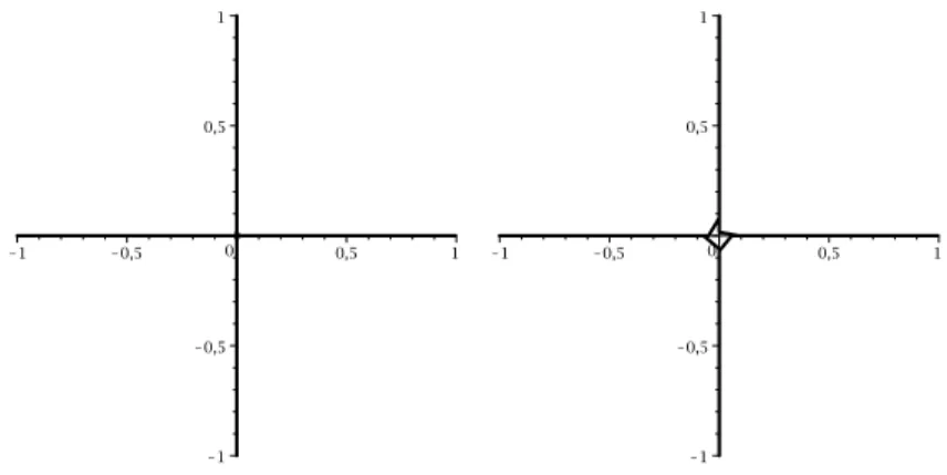
Example 2. Let Γ be a cross-like set, andµthe uniform measure onγ. The Riemann map is
φ(z) = p
a2(z2+ 1)2+b2(z2−1)2
2z ,
where aand b are the length of the horizontal and vertical semi-axis, respectively. In the particular case ofa=b,
φ(z) = a
√
2 2z
p z4+ 1.
The series expansion ofφis
φ(z) =
√
a2+b2
2 z+
−2b2+ 2a2 4√a2+b2
1 z +
√
a2+b2 µ
1 2 −
(−2b2+ 2a2)2 8 (a2+b2)2
2z3 + O
µ 1 z5
where the first coefficient
√
a2+b2
2 agrees with the capacity of the support. If a=b, the series expansion is
φ(z) =a
√
2 2 z+
a√2 4
1 z3 + O
µ 1 z5
¶ .
The image underφof the unit circle is shown in Figure 1, where we have included on the right the same result with an interpolation with less steps to give a better insight of the Riemann map.
Figure 1: φ(T) for a cross-like set
There are many instances, however, when the Hessenberg matrix can not computed completely, but only finite sections of it, and it is not possible to compute the limits of the diagonals of D. In this case, it is still possible to compute approximations of the support of the measure µ obtained computing the image of the unit circle under suitable approximations of the Riemann map. Specifically, since the coefficients of the Riemann map are the limits of the elements in each of the diagonals of the Hessenberg matrix, we may consider, as approximations of the Riemann mapφ, the functions
φk(z) =dk,k−1z+dk,k+
k−1 X
i=1 dk−i,k
zi ,
whereD= (di,j) is the Hessenberg matrix of µ[7].
Figure 2: φk(T) for k= 30, k= 40 and k= 50, respectively
Example 3. Consider now Γ an arc of circumference. In this case [10] (see also [17, 18]), there exists a measure for which the diagonals of the Hessenberg matrix stabilize from the second element on. The monic orthogonal polynomials associated to this measure satisfy Φ0(0) = 1 and Φn(0) = 1a (a > 1), if n≥1, and the corresponding Hessenberg
matrix it the following unitary matrix:
D= −1 a −
(a2−1)1/2
a2 −
(a2−1)2/2
a3 −
(a2−1)3/2
a4 −
(a2−1)4/2 a5 · · · (a2−1)1/2
a −
1
a2 −
(a2−1)1/2
a3 −
(a2−1)2/2
a4 −
(a2−1)3/2 a5 · · · 0 (a2−1)1/2
a −
1
a2 −
(a2−1)1/2
a3 −
(a2−1)2/2 a4 · · · 0 0 (a2−1)1/2
a −
1 a2
(a2−1)1/2 a3 · · · .. . ... ... ... ... . .. .
Hence we know the limits of the diagonals, and we can obtain the sum of these limits. It is easy to check thatD−T is compact and that the rows of T are in `1, and hence the expression of the Riemann map is
φ(z) = z ³
a−√a2−1 z´
√
a2−1−az
=
√
a2−1 a z−
1 a2 −
√
a2−1 a3z −O
µ 1 z2
¶ ,
Figure 3: φ(T) for an arc of circumference
In the following figure we compute several approximations of the support ofµ, for the particular case a = 2, using the above method, for k = 10, k = 20 and k = 30, respectively.
Figure 4: φk(T) for k= 10, k= 20 and k= 30, respectively
Example 4. In the following example we take Γ as the half part of a drop-like set of parametric equation
z(t) = (eit)2
1 + 2eit, t∈[0, π].
Figure 5: φk(T) for k= 5, k= 8 and k= 11, respectively
Example 5. For the last example we take Γ as the spiral with parametric equation
z(t) =teit
6 , t∈[0,2π]
and we consider µ the uniform measure on γ. In the following figure we show sev-eral approximations of the support of µ using this method, for k = 1 and k = 12, respectively.
Figure 6: φk(T) for k= 1 and k= 12, respectively
Acknowledgements
The authors have been supported by Comunidad Aut´onoma de Madrid and Universidad Polit´ecnica de Madrid (UPM-CAM Q061010133).
References
[2] M. Bello and G. L´opez, Ratio and relative asymptotics of polynomials orthogonal on an arc of the unit circle, J. Approx. Theory, 92 (1998) 216-244.
[3] A. B¨ottcher and S. M. Grudsky, Spectral properties of banded Toeplitz matrices, Siam, Philadelphia, 2005.
[4] T. S. Chihara, An introduction to orthogonal polynomials, Gordon and Breach, New York, 1978.
[5] J. B. Conway, A course in functional analysis, Graduate Texts in Mathematics, Springer-Verlag, New York, 1985.
[6] J. B. Conway, The theory of subnormal operators, Mathematical Surveys and Monographs, vol.36, AMS, Providence, Rhode Island, 1985.
[7] C. Escribano, A. Giraldo. M. A. Sastre y E. Torrano,Approximation of Riemann maps for Jordan arcs, Preprint.
[8] G. Freud, Orthogonal polynomials, Consultants Bureau, New York, 1961. [9] D. Gaier,Lectures on complex approximations, Birkh¨auser, Boston, 1985.
[10] L. Golinskii, P. Nevai and W. Van Assche,Perturbation of orthogonal polynomials on an arc of the unit circle, J. Approx. Theory83 (3) (1995) 392–422.
[11] L. Golinskii and V. Totik,Orthogonal polynomials: from Jacobi to Simon, in Spec-tral Theory and Mathematical Physics: A Festschrift in Honor of Barry Simon’s 60th Birthday, P. Deift, F. Gesztesy, P. Perry, and W. Schlag (eds.), Proceedings of Symposia in Pure Mathematics, 76, Amer. Math. Soc., Providence, RI, 2007, pp. 821-874.
[12] P. R. HalmosTen problems in Hilbert space. Bull. Amer. Math. Soc.76(5) (1970) 887–933.
[13] A. M´at´e, P. Nevai and V. Totik, Asymptotics for the ratio of leading coefficients
of orthonormal polynomials on the unit circle, Constr. Approx.1 (1985) 63-69.
[14] C. Pommerenke, Univalent functions, Vandenhoeck and Ruprecht in G¨ottingen, Studia Mathematica, 1975.
[15] E. A. Rakhmanov, On the asymptotics of the ratio of orthogonal polynomials, Math. USSR Sb.32 (1977) 199–213.
[16] E. A Rakhmanov, On the asymptotics of the ratio of orthogonal polynomials. II, Math. USSR Sb.47 (1983) 105–117.
[18] B. Simon, Orthogonal polynomials on the unit circle, Part 2: Spectral Theory, AMS Colloquium Publications, American Mathematical Society, Providence, RI, 2005
[19] H. Stahl and V. Totik, General Orthogonal Polynomials, Cambridge University Press, 1992.
[20] G. Szeg¨o, Orthogonal polynomials, American Mathematical Society, Coloquium Publications, Vol. 32, first ed. 1939, fourth ed. 1975.
[21] V. Tomeo, La subnormalidad de la matriz de Hessenberg asociada a los P.O. or-togonales en el caso hermitiano, Tesis Doctoral, Madrid, 2004.