Two-layer particle filter for multiple target
detection and tracking
Ángel F. García-Fernández, Jesús Grajal, Mark R. Morelande
Abstract
This paper deals with the detection and tracking of an unknown number of targets using a Bayesian
hierarchical model with target labels. To approximate the posterior probability density function, we
develop a two-layer particle filter. One deals with track initiation, and the other with track maintenance.
In addition, the parallel partition method is proposed to sample the states of the surviving targets.
Index Terms
Two-layer particle filter, parallel partition method, detection, tracking, target labels.
NOMENCLATURE
Pk Vector that contains the positions of all tracks at timek
pk
j,i ith position particle of trackj at timek
pk
j Position vector of track j at timek
Rk Augmented multitrack state vector j at timek
rk
j Augmented state vector of track j at timek
Xk+1 Sk
Multitrack state vector of the targets whose labels are in setSk at timek+ 1
Copyright (c) 2012 IEEE. Personal use of this material is permitted. Permission from IEEE must be obtained for all other
users, including reprinting/ republishing this material for advertising or promotional purposes, creating new collective works for
resale or redistribution to servers or lists, or reuse of any copyrighted components of this work in other works.
Ángel F. García-Fernández was supported by an FPU Fellowship from Spanish MEC. This work was supported in part by
the Spanish National Research and Development Program under Projects TEC2011-28683-C02-01 and Comonsens
(Consolider-Ingenio 2010, CSD2008-00010). The authors would like to thank Wei Yi for helpful comments.
*Ángel F. García-Fernández and Jesús Grajal are with the Departamento de Señales, Sistemas y Radiocomunicaciones, ETSI
de Telecomunicación, Universidad Politécnica de Madrid, Ciudad Universitaria s/n, 28040 Madrid, Spain. email: {agarcia,
jesus}@gmr.ssr.upm.es. Mark R. Morelande is with the Department of Electrical and Electronic Engineering, The University of
xk+1 skj State vector of the target whose label is skj at timek+ 1
Xk Multitrack state vector at timek
xk
j State vector of trackj at timek
xk
j,i Rao-Blackwellisedith particle of track j at timek
z1:k Sequence of measurement vectors from time 1 tok
zk Measurement vector at timek
bk Number of targets that are born at timek dk Number of targets that die at time k Ik Set of labels at timek
Nk Set of labels of the targets that are born at time k
Sk Set of labels of the targets that survive from time ktok+ 1 tk Number of tracks at time k
I. INTRODUCTION
The random finite set (RFS) framework has emerged as a natural way to perform multiple target detection and tracking from the Bayesian point of view [1]. In the RFS framework, the multitarget state is a set whose elements are single target state vectors. Densities within the RFS framework are manipulated using rules analogous to those which are applied in vector-based approaches [2]. Thus, the (unnormalised) RFS posterior density can be found using an RFS analog of the Chapman-Kolmogorov equation followed by multiplication of the result by an RFS version of the likelihood. Importantly, this framework permits the development of rigorous metrics for algorithm performance assessment [3], [4]. In the usual case of RFS, the state vectors do not include identifying labels and, therefore, we estimate the target number and target states without connecting these estimates, instant to instant, into temporally connected tracks [5].
the posterior remains unchanged under target permutations [9, Appendix B]. This leads to a theoretical inconsistency since the Bayesian filtering recursion for vector-valued variables does not generally provide the required symmetry [10]. Rather, this symmetry must be imposed. The resulting JMPD actually ends up being equivalent to the RFS posterior but is not satisfying theoretically. As such, the RFS framework should be used if individual target states are not labelled.
The essential task of linking target state estimates along time to form tracks can be done if a unique label is added to each single target state in both approaches. Labels differ from the usual kinematic parameters in two important ways: they are unique (no two tracks can have the same label) and they are fixed in time. Track construction through labelling has been proposed in several papers, although usually with ad hoc approaches. In [7] labels are added in the particle filter (PF) approximation to the JMPD but they are not included in the Bayesian model. The same happens in the PF approximation to the probability hypothesis density (PHD) filter, which is an approximation to the full RFS posterior, proposed in [11]. As labels are included in the target state, a principled approach must take them into account directly in the Bayesian model not in an approximation to a theoretically unlabelled density. An example of this principled approach to track labelling within the RFS framework can be found in [12]. It is important to note that the two distinguishing characteristics of the labels imply some important changes with respect to the unlabelled target case. As pointed out in [9, Appendix B], now there is a bijection between the multitarget RFS and a hybrid state formed by the target number and a multitarget state vector with labels. Therefore, because of this one-to-one correspondence, both representations lead to the same results and, importantly, they are equally sound. Additionally, this one-to-one correspondence implies that any metric defined in an RFS framework can be equivalently defined in this framework. Since a vector-based approach with labels conveys the same information as an RFS approach with labels we will pursue the former approach because some parts of this paper are clearer this way. Nevertheless, this paper could have been written using RFS notation as they are equivalent. We note that hierarchical models of the type used here have been previously used in multitarget tracking in [13] and, more generally, are commonly used in Bayesian inference [14]–[16].
paragraphs discuss existing work on these problems and summarise how the proposed methods address the limitations of these approaches.
An important property of the measurement model commonly used in multitarget tracking is the approximate factorisation of the likelihood. This factorisation depends on the measurement model but usually applies for widely separated targets. As a result of this property only the states of targets which form clusters based on proximity need to be sampled jointly. This effectively reduces the dimensionality of the sampling problem. This idea was first exploited for sequential importance sampling in [18] and also used in [6]–[8], [19]–[21]. Although distant targets can be ignored it is desirable that samples of targets within a cluster be sampled jointly. This was achieved in [7] by jointly sampling clusters of target states from the optimal importance density (OID) [22]. The OID is not universally applicable because it is generally intractable although approximations to the OID using a bank of extended or unscented Kalman filters have been proposed [22], [23]. However, jointly sampling from the OID, or an approximation, can be computationally expensive, even for relatively small clusters of targets. The aim is therefore to construct an importance density which considers the presence of neighbouring targets in a computationally efficient manner. The proposed parallel partition (PP) method achieves this aim by a simple modification of the independent partition (IP) method of [6]. PP is a general method in the sense that it does not rely on a specific measurement model that is intended to improve the efficiency of sampling of the target states, especially when the number of particles is low and a fast algorithm is required under the assumption that tracks are a priori independent. In addition, we show that what the well-known IP method really does is sampling an auxiliary vector, therefore, providing more insight into multiple target tracking using PFs.
existing track if appropriate, while the LRT for the existing tracks determines target removal. Then, the PF developed in this paper has a two-layer scheme in which the posterior density of one layer is used to specify the importance density of the other layer to sample newborn target states. A similar idea, although not in the context of importance sampling, is used in the integrated probabilistic data association filter (IPDAF) and its generalisations where a target existence probability is used to determine the track status [27]. Nevertheless, the idea of using an subsidiary PF to sample the newborn target states is a new idea developed in this paper.
The rest of the paper is organised as follows. In Section II, we address the joint multitrack probability density (JMKPD) and describe the models of targets and measurements. In Section III, we explain the PP method for fixed and known number of targets. The two-layer PF for variable and unknown number of targets is presented in Section IV. Numerical examples examining the filter performance are provided in Section V. Finally, conclusions are drawn in Section VI.
II. JOINTMULTITRACK PROBABILITYDENSITY
This section deals with the JMKPD [28], the target model and the sensor model. Basically, the JMKPD corresponds to the approach used in [13] but augmenting each target state with a unique label so that the tracks are perfectly identified along time. Adding the unique labels to each track enables us to use an equivalent representation in which the dimension of the state is governed by the number of elements of a set that includes the labels so that the required PDFs are written in a more compact form. As noted in the Introduction, and shown in [9, Appendix B], the JMKPD is equivalent to the RFS posterior density of the multitarget state with labels.
We assume there are tk tracks at time k. The state of track j at time k is described by vector
xk
j =
h
xk
j, .
xkj, yk
j, .
ykjiT ∈ R4 where pk
j =
h
xk
j, yjk
iT
is the position vector, vk
j =
h.
xkj,y.kjiT is the velocity vector and superscript T means transpose. The augmented state of track j is described at time
k by vector rkj =
xkjT, ikj
T
∈ R4 ×
N where ikj is the label of track j. It is imposed that ik1 <
ik2 < ... < iktk to ensure unique labelling of the tracks. The augmented multitrack state vector is formed
by stacking the individual augmented track state vectors into one vector Rk =h rk1T
, ..., rktk
TiT
=
h xk1T
, ik1, ..., xktk
T
, iktk
iT
. Since the number tk of targets is unknown, the variable
Rk, tk∈
∞
[
t=0
R4×Nt× {t}: ik1 < ik2 < ... < ikt.
Following [13], [29], the set R0 = {θ} where θ is a symbol for no target. A similar convention is
number) of the multitarget state [14]–[16].
The state at timekis observed through the measurement vectorzk. In a Bayesian framework, estimation of Rk, tk
based on the sequence of measurements z1:k= z1,z2, ...,zk
up to time k is achieved by the recursive computation of the posterior PDF p Rk, tk
z1:k
=p tk z1:k
p Rk
z1:k, tk
which is normalised such that
∞
X
tk=0
p tk z 1:k ∞ X ik 1=1 ... ∞ X ik tk=i
k tk−1+1
ˆ
dxk1...dxktkp
Rk z
1:k, tk= 1 (1) The explanation for the normalisation given in (1) is the following. In a Bayesian hierarchical model, firstly, we sum over all the models tk∈ {0} ∪N and then we integrate the state for that model. As the labels are discrete variables a sum is performed rather than a integral. In addition, the sum over the labels in (1) takes into account thatik1 < ik2 < ... < iktk, which ensures unique labelling.
The posterior is calculated recursively in two phases: prediction and update [30]. The prediction phase makes use of the Chapman-Kolmogorov equation:
pRk, tk
z
1:k−1
=
∞
X
tk−1=0
∞
X
ik1−1=1
...
∞
X
iktk−−11=i
k−1
tk−1−1+1 ˆ
dxk1−1...dxktk−−11p
Rk, tk
R
k−1, tk−1pRk−1, tk−1 z
1:k−1 (2)
The explanation about why (2) has this form is the same as for (1). The update equation is obtained by Bayes’ rule:
p
Rk, tk
z
1:k∝pzk R
k, tkpRk, tk z
1:k−1 (3)
It should be noted that PFs only require the posterior PDF up to a normalising constant [30]. Therefore, the normalisation constant is not included in (3) as it is not necessary in the PF implementation explained in the rest of the paper. When tk−1 = 0, Rk−1 can only take the value θ, thus, it is a discrete state so the integrals in (2) come down to a substitution of the probability mass of that state.
In the following, we introduce an equivalent notation that simplifies the writing of the necessary PDFs involved in (2) and (3). Let us define the variable Xk, Ikwhere Xk=
h
xk1T, ..., xktk
TiT
∈R4tk
is the multitrack vector and Ik = ik1, ik2, , ..., iktk is the set of labels. Now, it is the size of Ik that
governs the dimensionality of Xk. It is shown in [9, Section 4.2] that there is a one-to-correspondence between Xk, Ikand Rk, tk. This implies that computingp Xk, Ikz1:k
is equivalent to calculating
p Rk, tkz1:k
Table I – Equivalent notations for multitarget tracking with labels
Notation Quantity of interest
Hierarchical model with labels [13] Rk, tk=
h xk1
T
, ik1, ..., xktk
T
, iktk
iT
, tk
JMKPD [28] Xk, Ik=
h
xk1
T
, ..., xktk
TiT
,
ik1, i
k
2, , ..., i
k tk
RFS with labels [2]
h
xk
1
T
, ik
1
iT
, ...,h xk tk
T
, ik tk
iT
account that the RFS notation uses set densities and set integrals [2]. Nevertheless, this paper is written using the JMKPD for two reasons: using sets for the labels enables us to write the transition PDFs in a more compact form than using the hierarchical model in [13] and using vectors for the multitarget state enables us to describe the PP method in Section III in a more compact form than using sets.
Our aim is to computep Xk, Ikz1:k
recursively. To this end, we need to calculate (2) and (3) using a target transition PDF p Xk, IkXk−1, Ik−1
and the PDF of the measurement given the multitarget state p zkXk, Ik
, which are analogous to their representation using the variable Rk, tkand can be also written in the RFS framework. These are explained in the following subsections.
A. Multitrack model
This model is mainly the one in [28]. The model takes into account the births, deaths and motions of the targets. We assume that the a priori evolution of the number of targets in track is modelled by an
M/M/∞ birth-death process [31] with parameters, λ, the a priori arrival rate of targets, and 1/µ, the average life of a target. The a priori arrival rate of targets λ is taken to be proportional to the area AS of the surveillance region, λ=λAAS, whereλA would denote the prior arrival of targets per area unit. According to this model, the probability thatbk new targets appear at time k:
pbk= e
−λτ(λτ)bk
bk! (4)
where τ is the sampling interval [32]. The probability that a target dies in a sampling interval is:
pd= 1−e−µ·τ (5)
We define the sets: Sk=sk1, s2k, ..., sktk−dk the set of labels of the targets that survive from time k
tok+ 1wheredk is the number of targets that die at timekandNk+1=
n
nk1+1, nk2+1, ..., nkbk+1+1
o
the set of labels of the targets that are born at time k+ 1 soIk+1 =Sk ∪ Nk+1. We use Xk+1 Skto denote the components of the vector Xk+1 that correspond with the set of tracks in Sk. That is, Xk+1 Sk=
h
xk+1 sk1T, ... xk+1 sktk−dk
TiT
wherexk+1
skj
=
h
xk+1
skj
,x˙k+1
skj
, yk+1
skj
,y˙k+1
skj
represents the state of a target whose label is skj at time k+ 1 and sk1 < sk2 < ... < sktk−dk to ensure
unique ordering. Therefore:
pXk+1, Ik+1
X
k, Ik=pXk+1Sk, Sk,Xk+1Nk+1, Nk+1 X
k, Ik (6) Equation (6) comes from the fact that each component ofXk+1is either inXk+1 SkorXk+1 Nk+1
andIk+1=Sk ∪ Nk+1. Using the same procedure as in [28], equation (6) can be written as:
p
Xk+1, Ik+1
X
k, Ik=pNk+1pSk I
kpXk+1Nk+1 N
k+1pXk+1Sk X
k, Sk (7) Now we give the expressions for all the probabilities in (7) and explain their meaning. The first probability indicates how the new labels are assigned. To this end, let us partition the surveillance area
V ⊂R2 intoM cells of the same size V
1, V2, . . . , VM. Assume that at most one target can appear in a
given cell at a given sample time. The target appearing in the jth cell at thekth time is given the label
j+ (k−1)M. Let Fk = {(k−1)M+ 1, . . . , kM} denote the set of all possible labels that can be assigned at time k. Then
p
Nk+1
∝
p bk+1 ifNk+1⊆Fk+1
0 otherwise
(8)
where we should recall that Nk+1
=bk+1. It should be noted that we also use a grid on M sensors
in the measurement model to be described in Section II-B. However, this does not imply that this way of assigning the target labels can only be applied to this kind of measurement model. In general, for any measurement model, we can partition the surveillance area such that only one target can appear in a given region at a given time step.
The second probability in (7) indicates the set of labels of the targets that survive time k:
p
Sk
I
k=
Qtk
j=1
h
χSk
ikj
(1−pd) +
1−χSk
ikj
pd
i
ifSk ⊆Ik
0 otherwise
(9)
where χS(B) = 1 if B ⊆ S and zero otherwise and it has been assumed that each target dies with a probability pd independently from the rest.
The third probability in (7) indicates the a priori state of the targets that are born at timek. We assume that the states of newborn targets are independent and targetnk
j appears in cellVnk
j with an initial position
uniformly distributed in this cell and an initial velocity distributed following a PDF pv0(·). Therefore
pXkNk
N
k= bk Y
j=1
UVnkj
xknkj, yknkj·pv0
˙
where UVnk
j
(x, y) is a uniform random variable in the cellVnk
j, whose area isAnkj =AS/M (AS is the
area of the surveillance region), evaluated at (x, y).
The fourth probability in (7) is the dynamic model, a nearly constant velocity model [33]:
p
Xk+1
Sk
X
k, Sk= tk−dk
Y
j=1
N xk+1
skj
;Fxk
skj
,Q
(11)
F=I2⊗
1 τ
0 1
(12)
Q=σ2uI2⊗
τ3/3 τ2/2
τ2/2 τ
(13)
where it is assumed that the targets move independently, N(x;x,Q) is the Gaussian PDF evaluated at
xwith mean xand covariance matrix Q, Im is the m × m identity matrix,⊗is the Kronecker product andσ2u is the continuous-time process noise intensity [33].
B. Measurement models
We consider two measurement models. The first model is the pixellised image model commonly used in track-before-detect algorithms, where each pixel (sensor) corresponds to the received power in a particular spatial location [3], [6], [7], [34]. This model is used to compare our algorithm with the existence grid [7], [25] as to the creation and deletion of tracks. The other is a centralised sensor network in which the sensors are deployed in a surveillance area, measure the received power from emitting targets and transmit its value to a fusion centre, which carries out detection and tracking tasks [35]. Both models only differ in how the signal-to-noise ratio SN R at each sensor/pixel is calculated.
For the pixellised sensor model, the signal-to noise ratio produced by a target with coordinates[x, y]T
in a pixel (sensor) is [7]:
SN R(x, y, xs, ys) =
SN R |x−xs| ≤lx/2 and |y−ys| ≤ly/2
0 otherwise
(14)
where [xs, ys]T are the coordinates of the sensor and [lx, ly]T is the size of the pixels.
respectively. Therefore:
SN R(r) =
SN Rr,1 0≤r < r1
... ...
SN Rr,N rN−1≤r < rN
0 r≥rN
(15)
which can approximate any isotropic propagation model as accurately as possible.
For both models we assume that there are M sensors located in the surveillance area with the vector
zk =
zk
1, z2k, ..., zMk
T
containing the measurements from each sensor which are independent in each sensor. We assume Rayleigh-distributed measurements. This distribution corresponds to envelope-detected signals under a Gaussian model. This model has been used in radar systems [26] and radio signal propagation [36]. Then, the PDF of the measurement at sensor j conditioned on the current multitarget state depends on the total signal-to-noise ratio at sensor j, SN Rj, which is the sum of the signal-to-noise ratios produced by each target [37], calculated using (14) or (15) depending on the sensor model. Therefore:
p
zk
X
k, Ik= M
Y
j=1
p
zkj |SN Rj
(16)
where the dependency of SN Rj on Xk is not given explicitly. The PDF of the measurement for sensor
j for non-thresholded data is:
pzkj |SN Rj
= z
k j
1 +SN Rj
exp
−
zjk2
2 (1 +SN Rj)
(17)
In the numerical simulations in Section V, we also analyse the effect of thresholding the data on performance as in [6], [7]. This binary data (detections) is obtained using thresholdΓ:
Γ =p−2 lnPf a (18)
where Pf a is the false alarm probability per sensor. Then, the PDF of the measurement for sensor j for binary data is:
pzjk|SN Rj
=P1/(1+SN Rj)
f a δ
zkj −1+1−P1/(1+SN Rj)
f a
δzjk (19)
III. PARTICLE FILTER IMPLEMENTATION FOR A FIXED AND KNOWN NUMBER OF TRACKS
In this section, we present a PF to approximately solve (2) and (3) when the number of tracks is fixed and known. We will generalise the algorithm for a variable and unknown number of tracks in the next section. In this case, the number of tracks over time is constant tk = t, Ik = I = {1, ..., t} the set of labels of the surviving tracks coincides with the labels at the previous step Sk = I and no tracks are born at any time Nk = Ø. Therefore, the JMKPD comes down to estimating p Xkz1:k
as the labels are implicit in the ordering of the multitarget state vector Xk. In addition, as nonlinearity in our tracking model enters in the relationship between the measurements and the positions of the tracks and the relationship between the velocities and the positions is linear and Gaussian, the posterior of the velocity elements can be computed exactly using a Kalman filter conditional on the trajectory of the targets. This technique, known as Rao-Blackwellisation, improves the filter performance for a given sample size [7], [38]. Then, the Rao-Blackwellised PF approximation to the JMKPD at time k is approximated as [9]
p
Xk
z
1:k≈ Npar
X
i=1
wikδ
Pk−Pki Yt
j=1
p
vkj
p
0:k j,i
(20)
where
p
vkj
p
0:k j,i
=Nvkj;vkj,i,Σkj,i
(21)
andNpar is the number of particles,wki is the normalised weight of particleiat timek,Pk is the vector that contains the positions of all tracks at timek,Pki is theith particle at timek, andvkj,i andΣkj,iare the posterior mean and covariance matrix of the velocity elements conditional on the trajectory of positions for theith particle andjth trackp0:j,ik. At timek, what we need to store is the Rao-Blackwellised particles
Xki =
Pki,vk1,i,Σk1,i, ...vkt,i,Σkt,i
for i= 1, ..., Npar.
The PF approximation of the posterior density of the positions at time k+ 1 using Bayes’ rule and (11) in (20) and integrating out the targets’ velocities at time k+ 1is [9]:
pPk+1
z
1:k+1∝pzk+1 P
k+1
Npar X
i=1
wki
t
Y
j=1
ppkj+1
x
k j,i
(22)
wherexkj,i is the Rao-Blackwellised ith particle of trackj at time kandp
pkj+1
x
k j,i
is Gaussian with mean pkj,i+τvkj,i and covariance matrix τ2Σkj,i+Qp where Qp is the process noise covariance matrix for the position elements according to (13).
We propose an importance density constructed using a method called parallel partition (PP). The method developed here is a convenient, fast way to propagate particles in multitarget situations.
A. Parallel Partition method
Here, we propose the PP method as a modification of the well-known IP method and provide a detailed mathematical explanation on how both methods work via auxiliary sampling. IP and PP methods make the following assumption:
Assumption 1. Tracks are a priori independent with evenly distributed weights, wik= 1/Npar, so that
p
Pk+1
z
1:k∝ t Y j=1 Npar X i=1 p pkj+1
x k j,i (23)
The proof of (23) under Assumption 1 can be found in the Appendix. Under Assumption 1, the posterior PDF becomes:
p
Pk+1
z
1:k+1∝pzk+1 P k+1 t Y j=1 Npar X i=1 p pkj+1
x k j,i (24)
We should note that getting weights evenly distributed at timekcan be done by performing a resampling step of the particles at time k[30].
Then, what we propose is to sample an auxiliary variable for each track such that the posterior is:
pPk+1,a
z
1:k+1∝pzk+1 P
k+1
t
Y
j=1
ppkj+1
x k j,aj (25)
where a = [a1, ..., at]T ∈ {1, ..., Npar}t and aj indicates that we are choosing the component aj for trackj on the mixture given by the prior, see equation (24). The idea of sampling in a higher dimension has traditionally been used, for instance, in the auxiliary PF, and can provide a lot of benefits [22], [30], [39]. We should note that integrating out the auxiliary variables in (25), we get the PDF of (24) so this definition of auxiliary variables is sound. If we draw a sample from the joint density (25) and then discard the part of the sample that corresponds witha, then we are producing a sample from (24) as required.
If we draw Pki+1,ai =
ai1, . . . , aitT from an importance density q1(·) for i = 1, . . . , Npar, the
updated weights are calculated as:
wki+1 ∝
p
zk+1
P k+1 i Qt
j=1p
pkj,i+1
x k j,ai j q1
Pki+1,ai|z1:k+1
(26)
The importance density in the PP filter is taken to be:
q1
Pk+1,a z
1:k+1=
t
Y
j=1
bj
where
bj
pkj+1
∝p
zk+1
pˆ
k+1|k
1 , . . . ,pˆ
k+1|k j−1 ,p
k+1
j ,pˆ k+1|k
j+1 , . . . ,pˆ
k+1|k t
(28)
and pˆkj+1|k is the predicted position of track j averaged over all the particles. We call bj
pkj+1
the first-stage weights. In contrast, we want to indicate that the IP method usesbj
pkj+1
∝p
zk+1
p k+1 j
rather than (28).
Substituting (27) and (28) into (26), the unnormalised particle weights, second-stage weights, are:
wik+1∝
pzk+1
P k+1 i Qt
j=1bj
pkj,i+1
(29)
The computational expense of evaluating (28) and then (29), can be lowered if we separate the tracks intos≤tclusters C1k+1, . . . , Ck+1
s such that
Ss
l=1Clk+1=I and∀l ∈ {1, . . . , s}, ∀i ∈C
k+1
l
ˆp
k+1|k i −ˆp
k+1|k j
≤Γc→j ∈C
k+1
l (30) whereΓcis a threshold. Equation (30) is a mathematical way to indicate that if the distance between the predicted positions of two tracks is below Γc, then, these tracks belong to the same cluster1. Using the same reasoning as in [7], for a sufficiently large value of Γc, we can write (28) as:
bj
pkj+1
∝p
zk+1
Cˆ
k+1|k l−{j},p
k+1
j
(31)
where Cˆkl−{+1j|k} are the predicted positions of the tracks that belong to clusterl, in which trackj is also included, except the position of track j averaged over all the particles.
In the rest of the section, we explain how we draw samples from (27) and provide a discussion about the proposed method.
1) Sampling from the importance density: Here, we explain how IP and PP draw samples from (27)
recalling that the only difference between both methods is the definition of bj
pkj+1
. We can write
q1
Pk+1,a z
1:k+1=
t
Y
j=1
q1,j
pkj+1, aj
z
1:k+1=
t
Y
j=1
bj
pkj+1ppkj+1 x k j,aj (32)
where q1,j(·) is the importance density to draw positions and indices for track j. It should be noted that it is generally not possible to sample directly fromq1,j(·). Instead, we use the approximate method sampling/importance resampling in [40] to get samples from q1,j(·).
1
a) General algorithm: According to [40], we can define a “first-pass approximation” of
q1,j
pkj+1, aj
z1:k+1
called h
pkj+1, aj
z1:k+1
. Then, we draw Mpar samples from
h
pkj+1, aj
z1:k+1
, which are denoted byp∗j,p, a∗j.p forp= 1, ..., Mpar, and we evaluate
r p∗j,p, a∗j.p∝
q1,j
p∗j,p, a∗j.pz1:k+1
h
p∗j,p, a∗j.p|z1:k+1 (33)
Finally, we draw Npar values of
pkj+1, aj
from the distribution defined by
p∗j,p, a∗j.p
for p =
1, ..., Mpar with probability proportional tor
p∗j,p, a∗j.p
. The resulting particles are samples fromq1,j(·) [40].
b) Application to IP and PP: In both IP and PP methods,h(·) is
h
pkj+1, aj
z
1:k+1∝ppk+1
j x k j,aj (34)
and IP and PP sample fromh(·)via stratified sampling [41]. The sample space of
pkj+1, aj
isΩ =R2×
{1, ...Npar}. Then, we can defineNpar disjoint subregions
D1, ...,DNpar such thatDi=R
2× {i}and
Ω =SNpar
i=1 Di. From (34), the probability that a sample belongs to regionDi is1/Npar, i.e., the regions are equally probable. Then, assuming we wantMpar samples fromh(·), there areMi samples in region
Di such thatPNi=1parMi =Mpar. Since the variance in these regions is the same, the optimal way to assign
Mi isMi =Mpar/Npar [41] . In the IP and PP methodMpar =Npar, soMi =Npar/Npar= 1although it can be easily generalised forMpar > Npar. This implies that sampling from h
pkj+1, aj
z1:k+1
can be done going through all the regions (i.e. indices of the particles), drawing one position per each region (particle), noting that in each region the index is deterministic.
Once we have Mpar samples from (34), we draw Npar values of
pkj+1, aj
from the empirical distribution defined over the values
p∗j,p, a∗j.p
for p = 1, ..., Npar with probabilities proportional to
r
p∗j,p, aj.p
= bj
p∗j,p
getting samples from q1,j(·). These are the steps shown in Table II. We should mention that in [18] and [6] they also sample following the steps in Table II but they do not justify why.
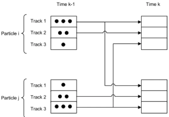
2) Discussion about the PP method: The important features of the PP method are subparticle crossover
and the way the first-stage weights are chosen. By “subparticle” we refer to the part of a particle that represents a single track. Therefore, a particle is made up of the subparticles of all the tracks. Then, by sampling an auxiliary variable for each track,ain (27), what we are doing is that a particle at time stepk
is formed by the propagation of subparticles that belonged to different particles at time k−1, see Figure 1. For example, a certain ai =
ai1, . . . , aitT indicates that to form particle iwe are using subparticle
Table II – Independent and Parallel Partition Subroutines
IP and PP subroutines for track or pre-trackjwith Rao-Blackwellisation
• For each particlei= 1, ..., Npar (RegionDi):
– Get a sample for the positionp∗j,ivp pkj+1
xkj,i
using (11).
– Calculate the mean and covariance matrix of the velocity using a Kalman filterv∗j,i yΣ
∗
j,i.
– IF we are using IP
∗ Calculatebj p∗j,i
=p zk+1
p
∗
j,i
using (16).
– ELSE (we are using PP)
∗ Calculatebj p∗j,i
=pzk+1
p
∗
j,i,Cˆ k+1|k l−{j}
using (16) wherelis the cluster of trackj.
• Normalisebj p∗j,i
to sum to one overi= 1, ..., Npar.
• Resampling step for each track. For each particlei= 1, ..., Npar:
– Sample an indexpfrom the distribution defined bybj p∗j,l
overl= 1, ..., Npar.
– Setxkj,i+1=
p∗j,p,v¯
∗
j,p,Σ
∗
j,p and the parent’s indexaij=p.
Time k-1 Time k
Particle i
Particle j Track 1
Track 2
Track 3
Track 1
Track 2
Track 3
Figure 1 – Subparticle crossover for three tracks: A particle at time k can be made up of the propagation of the tracks that belonged to different particles at time k−1. The circles inside each subparticle stand for the first-stage weight of the subparticle, see (31). At timek, we tend to form particles with subparticles that have a high first-stage weight. In this case, ai = [i, i, j]T andaj= [i, j, j]T.
Subparticle crossover is also included in the IP method [6], [8], [19]. In fact, as we indicated, the IP method is equivalent to the PP method if the first stage weights are given bybj
pkj+1
∝p
zk+1
p
k+1
j
high likelihood when considering all the targets together.
It should be noted that Assumption 1, which is required for subparticle crossover, does not necessarily hold for a group of closely spaced tracks as their positions conditioned on the measurements could be dependent. However, assumptions of this kind are quite common in multitarget tracking algorithms. For instance the well-known joint probabilistic data association filter (JPDAF) [42] assumes a priori independence of the target states as does the Monte Carlo approximation to the JPDAF proposed in [23]. These methods have been shown to work very well despite the occasional invalidity of this assumption. Using Assumption 1 when it is not satisfied can be interpreted as a way of trading-off bias and variance. In particular, we argue that the bias incurred in assuming a priori independence when it does not actually exist is less than the variance which results by the joint sampling of several track states, particularly when tracks states are sampled from the prior and the number of particles is relatively small. This was proved in [43] for the case of a Gaussian posterior.
We also want to highlight that the PP method can be used for any measurement model as it only requires Assumption 1, which is independent of the measurement model. Here, PP has been explained using Rao-Blackwellisation but this is not an essential part of the algorithm. As in Bayesian filtering the likelihoodp zk+1Xk+1
is always available, PP can always be used as it only requires to sample from the prior and evaluate the likelihood as indicated previously.
IV. PARTICLE FILTER IMPLEMENTATION FOR A VARIABLE AND UNKNOWN NUMBER OF TRACKS
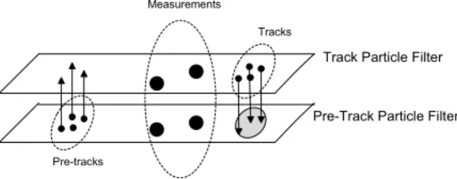
In the previous section we presented the PP method as a way to propagate particles in a multitarget tracking set-up when the number of targets is fixed and known. In this section, we present a two-layer PF to deal with the problem of tracking a variable and unknown number of targets. One layer deals with the termination of the tracks and the tracking itself while the other deals with track initiation. Both layers are PFs on their own, therefore, they are called track PF and pre-track PF, respectively. This idea is illustrated in Figure 2.
Firstly, we describe the importance density for the track PF. The importance density is chosen so that it factorises as:
qPk+1, Ik+1,a,c
z
1:k+1=q
p
Pk+1Sk, Sk,a z
1:k+1q 3
Pk+1Nk+1, Nk+1,c z
1:k+1
(35) wherea= [a1, ..., atk]T is the auxiliary vector of the PP method and,c= [c1, ..., cbk+1]T ∈ {0, ..., Npar}b
k+1
Track Particle Filter
Pre-Track Particle Filter Measurements
Pre-tracks
Tracks
Figure 2 – Two-layer PF diagram. The measurements update the two layers simultaneously. When the
pre-tracks are considered pre-tracks, they pass to the upper layer. In the area where there is a track, we do not initiate
pre-tracks.
importance density qp(·) propagates the labels of the surviving targets and their states. The importance density q3(·) proposes the positions of the tracks that are born at time k+ 1 and assigns their labels.
The importance density qp(·) is taken to be:
qp
Pk+1Sk, Sk,a z
1:k+1=q 1
Pk+1,a z
1:k+1q 2
Sk
P
k+1,a,z1:k+1 (36)
where q1(·) is the importance function of the PP method for known number of targets, equation (27),
that only depends on the particles at time k, and q2(·) determines the survival targets at time k and is
defined as:
q2
Sk
P
k+1,a,z1:k+1=
tk Y
j=1
h
q2,j
ikj,aj ∈Sk
p
k−Nd+2:k+1
1,a1 , ...,p
k−Nd+2:k+1
tk,a
tk ,z
k−Nd+2:k+1
χSk
ikj,aj
+
1−q2,j
ikj,aj ∈Sk
p
k−Nd+2:k+1
1,a1 , ...,p
k−Nd+2:k+1
tk,a
tk ,z
k−Nd+2:k+1 1−χ
Sk
ikj,aji (37)
where q2,j
ikj,a
j ∈S
k represents the probability that track ik
j,aj survives, p
k−Nd+2:k+1
j,aj represents the
trajectory of particle aj of target j from time k−Nd+ 2 to k+ 1. Thus, Nd is the number of past time steps that we use to decide if a track survives. We make q2(·) dependent on several time instants
so that we take into account the target’s dynamics to remove targets. In Section IV-A, we explain this importance function thoroughly.
Finally, the importance density for sampling the states of newborn tracksq3 Pk+1 Nk+1
, Nk+1,cz1:k+1
A. Importance density for removing tracks
The removal of a track in a particle is performed via a likelihood ratio test (LRT) [44] based on Nd time instants as indicated by (37). The decision to remove a track considers several time instants so that we take into account target dynamics. The two hypotheses for the test are H1: the track ikj is alive and
H0: the trackikj is dead. In [28], the algorithm considered each target alone in the surveillance area but that is a simplification because the decision to remove a track should take into account nearby targets. Due to the fact that the importance density has to be non-zero wherever the prior is, we need to define an acceptance probability for the result of the test:
q2,j
ikj ∈Sk
P
k−Nd+2:k+1,zk−Nd+2:k+1
=
Pa Λd=H1
1−Pa Λd=H0
(38)
where Pa is the probability of accepting the hypothesis given by the test2 and Λd is the LRT [44], assuming that track ikj belongs to cluster lk at timek:
QNd−2
l=−1 p
zk−l
C
k−l lk−l
QNd−2
l=−1 p
zk−l
Ck−l
lk−l−{ik j}
Λd=H1
≷
Λd=H0
ηd (39)
where ηd is a threshold,Cklk represents the positions of the tracks in clusterlk at time k and Ck
lk−{ik j}
represents the positions of the tracks in cluster lk at time k except the position of track ikj.
B. Importance density for sampling newborn track states. Pre-track particle filter
As we stated previously, the importance density for sampling the states of the newborn tracks,q3(·)in
(35), is built by means of a subsidiary PF. This PF is referred to as pre-track PF because it deals with the initialisation of tracks. The pre-track PF approximatesp
˜
Xk,I˜kz1:k
whereX˜k and I˜k stand for the multitrack state vector and set of labels of the pre-tracks. Based on an LRT, it is decided which of these pre-tracks are real and, consequently, are used to build the importance density q3(·). As it is another PF,
we must specify the a priori model, the measurement model and the importance density of the pre-tracks as done with the tracks in Section II. The measurement model and the state evolution model are the same as in Section II except for the births and deaths of pre-tracks, equations (4) and (9). This is explained in the following.
2We mainly useP
a for theoretical reasons but we actually accept the output of the LRT in the simulations. This could be
1) Birth and death of pre-tracks: The initialisation of pre-tracks in a sensor region is done as follows. First, that sensor and its neighbours must not have tracks or pre-tracks in their area of influence (area in which a target produces anSN R above zero). Second, if we are using binary sensors, there has to be a detection in that sensor or if we are using non-thresholded data sensors, the measurement in that sensor has to be higher than the threshold in (18) given Pf a. In this subsection, we name these two events as false alarms for the sake of clarity. Hence, for non-thresholded and binary data,Pf a is the probability of initiating a pre-track in a sensor which does not have any targets in its surroundings. It should be noted that if we do not use a grid-type measurement model as the ones used in this paper, we could devise a similar procedure to initiate pre-tracks using the regions for labelling described in Section II.
A pre-track can be initiated because of two independent events: the arrival of a real target, modelled by (4) and the occurrence of a false alarm. The probability mass function of the number of false alarms
nPf a in each sampling period is a binomial distribution that, under the assumption that Pf a 1 and
M 1, where M is the number of sensors, can be approximated by a Poisson random variable [28]:
p nPf a
≈ e
−M·Pf a(M·P
f a)nPfa
nPf a!
(40)
Then, the number of arrivals of pre-tracks in a time interval τ is the sum of two independent Poisson random variables, given by (4) and (40). The result is another Poisson random variable whose parameter is the sum of the parameters. Therefore, the probability that there are ˜bk births of pre-tracks is
p
˜
bk
≈
e−˜λ
˜ λ
˜bk
˜bk! (41)
where λ˜=λ·τ+M·Pf a.
It is considered for simplicity that the pre-tracks have a deterministic life equal to Nb instants of time.
2) Importance density for the pre-track PF: As with the track PF, the importance density of the
pre-track PF is split into three independent parts: dynamics, births and deaths of pre-pre-tracks. We make the following assumption:
Assumption 2. Newly appearing targets are well separated.
Due to Assumption 2, we use the IP method as the importance density for the evolution of the model
˜
q1(·). In view of the deterministic life of a pre-track, there is no need to define an importance density
˜
q2(·) because the pre-tracks are simply removed from the pre-track filter when they have lived for Nb time instants. The importance densityq˜3(·) used for the births of new pre-tracks works as follows: every
or a pre-track, a new pre-track is initiated with a position drawn from a uniform PDF in the area of the cell and the target velocity is initiated in a similar way as in Section V.C of [7]: When a pre-track is added to a particle of the pre-track layer, we draw two integers η1, η2 such that P (ηi=j) = 1/2 for
j∈ {−1,1} i∈ {1,2} and then select the initial distribution of the velocity to be Gaussian with mean
[η1, η2]T and covariance matrix 9I2.
3) Importance density for newborn tracks: Once a pre-track has lived for Nb time instants, an LRT
is carried out for each subparticle of that pre-track to decide whether it is a real track or not. The two hypotheses areH1: the pre-track is a real track andH0: the pre-track is a false track. Under Assumption
2, this test becomes:
QNb−2
l=−1 p
zk−l
H1,x˜
k−l˜ik j
QNb−2
l=−1p(zk−l|H0)
Λb =H1
≷
Λb =H0
ηb (42)
where ηb is the threshold and x˜k−l
˜ik j
denotes the state of the pre-track of label˜ikj at time k−l. Recall from (35) that sampling the states of the newborn tracks requires an auxiliary variable
c = [c1, ..., cbk+1]T ∈ {0, ..., Npar}b
k+1
where bk+1 is the number of pre-tracks in which at least one
subparticle has passed the test (42) at time k+ 1. The variable cj = 0 if the jth pre-track is discarded and cj 6= 0 indicates which subparticle from the pre-track PF is used to sample the state of a newborn track in the track PF.
The importance density q3(·) is taken to be:
q3
Pk+1
Nk+1
, Nk+1,c
z
1:k+1=
bk+1 Y
j=1
q3,1
cj
z
1:k+1q 3,2
pkj+1
z
1:k+1, c
j
q3,3
nkj+1
p k+1 j (43) where
q3,1
cj =i
z
1:k+1=
dj,i/Npar i6= 0
1−PNpar
i=1 dj,i/Npar i= 0
(44)
q3,2
pkj+1
z
1:k+1, c
j
∝p
zk+1
p k+1 j p pkj+1
x˜ k j,cj
cj >0 (45)
where x˜kj,i is the ith Rao-Blackwellised particle for pre-track j and dj,i is the output of LRT (42) for pre-track j and particle i, i.e., dj,i = 1 if Λb =H1 or dj,i = 0 otherwise. When cj = 0, it means that no target is born and, thus,q3,2(·) assigns pkj+1 =θ, whereθ is the symbol for no target [13]. Once we
have sampledcj for all the particles, the position of the new born target is sampled fromq3,2(·)using the
approximation in [40], i.e., via the IP method in Table II. In addition,q3,3(·) assigns the labels of these
and depends on the position of the new born target and the time index. Therefore, q3,3(·) corresponds
with the prior assuming that the target positions in all the particles lie in the same cell so that the target has the same label in all the particles.
One should note that the probability of transferring pre-track j to a particle in the track PF is
q3,1 cj >0
z1:k+1
= PNpar
i=1 dj,i/Npar = npass/Npar where npass is the number of particles that
have passed the test (42). Therefore, the more particles there are that pass the test, the more likely it is to initiate a track. In addition, the mean and covariance matrix of the initial velocity of a track are given by a Kalman filter that uses the past positions of the corresponding pre-track.
Then, using the prior model of evolution of targets and the measurement model in Section II and employing (35), (36), (38) and (43), the updated particle weights of the track PF are:
wik+1∝
pzk+1
P
k+1
i
p SikIik
pNik+1pPki+1Nik+1
N
k+1
i
q2 Sik
q3
Pki+1Nik+1, Nik+1,ci
Qtki
j=1bj
pkj,i+1
(46)
where the conditioning of the importance densities q2(·) and q3(·) has been removed to simplify the
notation and Sik and Nik+1 are the sets that contain the labels of the surviving targets and the new born targets of particle i, respectively. One should note that the prior PDF of initial target positions, given by (10), is inversely proportional toAbSk+1. On the other hand,pNik+1∝AbSk+1, recalling from Section II thatλ=λAAS. Then, both factors cancel each other out and the update of the weights is independent of the area of the surveillance region. Finally, a summary of the integrated detection and tracking algorithm is given in Table III.
V. SIMULATION RESULTS
In this section, we compare the proposed algorithm with other methods available in the literature. Firstly, we compare the PP method to other importance densities in the tracking part of the filter. Secondly, we compare the two-layer PF to other methods as for the estimation of the number of targets.
A. Tracking performance
The PP method is compared with other methods available in the literature: the above-mentioned IP, the adaptive proposal method that uses IP when the targets are far from each other and the coupled partition method (CP) when they are in close proximity3 [6], [8], a jointly auxiliary PF (JA) [39], [45], an adaptive auxiliary PF (AA) and the unscented Kalman filter (UKF) [46]. By JA, we denote the traditional auxiliary
3
Table III – Proposed algorithm for detection and tracking of multiple targets
• Separate the tracks into clusters using (30).
• For each track, sample the multiple track state using the PP method assuming all the targets survive, see Table II.
• Calculate the quotient of the LRT for the tracks using (39).
• For each pre-track, sample the multiple pre-track state using the IP method, see Table II.
• Calculate the quotient of the LRT for the pre-tracks using (42).
• For all the pre-tracks that have livedNbtime instants, evaluate the test (42).
– If there are pre-tracks that pass the test, sample the states of the newborn tracks using (43).
• For each particle in the track PF:
– Remove the tracks by evaluating the importance density (38).
– Update the weights of the particles using (46).
• Add pre-tracks to the pre-track PF according toq˜3(·), see Section IV-B.
• Update the weights of the particles in the pre-track PF, see Section IV-B.
• Perform resampling to obtain an evenly weighted particle set for both layers.
PF, i.e., at each time step we predict the multitarget state at the following time step, we compute the first-stage weights, we perform resampling and sample the multitarget state, see [39], [45] for details. JA never performs subparticle crossover. By AA, we denote an auxiliary PF that works by clustering of closely-spaced targets as in PP. Then, for each cluster we draw the particles using an auxiliary PF. Therefore, AA performs subparticle crossover for targets that are far, i.e., they do not belong to same cluster, and does not for targets that are in the same cluster. The properties of the importance densities of these PFs can be found in Table IV. The implementation of CP in our simulations uses R = 10
possible realisations of the future state as in [6]. The PFs have been implemented following the steps in Table III. The only part that changes is the importance density for sampling the surviving targets’ states. Our implementation of the UKF also makes use of the clusters. When the targets are isolated, we update their states and covariance matrices independently and when they belong to the same cluster we update all of them jointly. Thus, the number of sigma points that are needed to match the first two moments [46] is8Nc+ 1whereNc is the number of targets in the cluster4. A more detailed explanation of how the UKF can be used for the kind of measurement model we use in this paper is given in [45]. Our UKF implementation applies the LRT to the mean for track creation and removal. In addition, we have also implemented the algorithm described in [3], in which the posterior is approximated using
4
The dimension of the state of a target is 4. Consequently, the dimension of the state of a cluster is4Nc and therefore the
Table IV – Properties of the importance densities
Subparticle crossover (far) Subparticle crossover (near) Considers nearby targets
IP √ √ ×
CP √ × ×
PP √ √ √
AA √ × √
JA × × √
Table V – Simulation parameters
A priori model
λA 1/(100·τ·AS)
1/µ (133·τ)
σu 5m/s3/2
Filter (binary)
Nd 4
ηd 5·10−3
Nb 3
ηb 107
Filter
(non-thresholded)
Nd 4
ηd e−10
Nb 3
ηb e7
multi-Bernoulli random finite sets (MBRFS). The implementation of MBRFS in our simulations removes targets with existence probabilities below 0.001 and the initial existence probability for a target is 0.005. Note that other methods for multiple target tracking can only deal with thresholded measurements that require a data association step such as the algorithms given in [23], [47]–[51]. These algorithms cannot be directly applied to the measurement models described in Section II-B and, therefore, we do not provide comparisons with them.
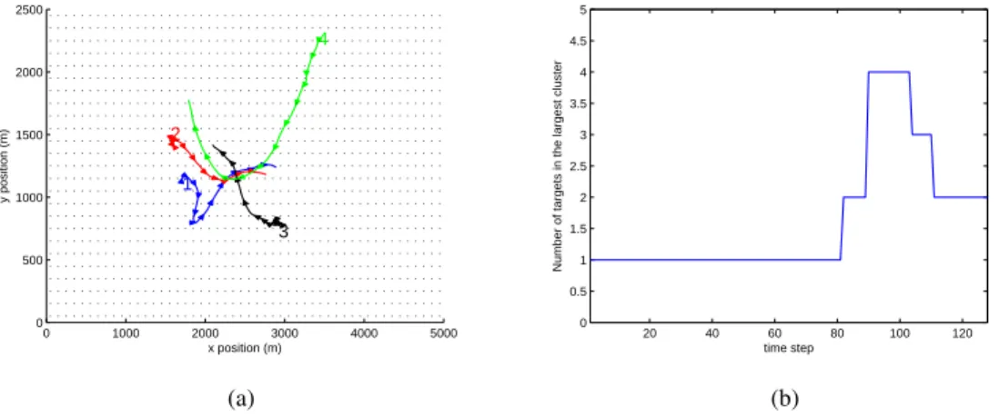
The scenario used to evaluate the performance of the algorithms consists of four targets whose trajectories cross at the same time, see Fig. 3. The sampling period of the trajectories is τ = 0.5 s
and there arel= 130time steps in the simulation. The targets appear at different times. The parameters used in the simulations are shown in Table V. The surveillance area is a rectangle whose dimensions are 5000 m ×2500 m. In this area, the sensors are arranged forming a grid of 50 ×25 sensors whose side is 100 m. Each cell of the grid is one of the regions V1, ..., VM defined in Section II-A. The SN R of a sensor produced by one target is approximated by a piecewise linear function:
SN R(r) =
20 dB r <60 m
10 dB 60 m≤r <80 m
0 r ≥80 m
(47)
0 1000 2000 3000 4000 5000 0
500 1000 1500 2000 2500
x position (m) y position (m) 1
2
3 4
(a)
20 40 60 80 100 120 0
0.5 1 1.5 2 2.5 3 3.5 4 4.5 5
time step
Number of targets in the largest cluster
(b)
Figure 3 – Simulation scenario: (a) target trajectories and (b) the largest cluster size for the true target positions
plotted against time for a clustering thresholdΓc = 200m. In (a), each target is identified at the beginning of its trajectory by a number and there is an arrow to indicate the target position every ten time steps. Target one
appears at time step 1, targets two and four at time step 3 and target three at time step 4. The targets do not
disappear until the end of the simulation. Black dots indicate the sensor positions.
We evaluate the tracking performance calculating the root mean square (RMS) of the position error by a Monte Carlo simulation with m= 50 realisations. To assess the tracking performance, we make a
Track-to-truth Assignment Table [26] in which each track is associated with one target or with none at
each time step depending on the distance from the track to the real position of the target and a threshold that is taken to be Λ = 120 m. If the distance from a track to a target exceeds that threshold, the track cannot be associated with that target. The threshold for forming the clusters is Γc= 200m. In addition, a track is assumed to be active if at least 70% of the particles contain it.
Let ˆpki (j), i= 1, . . . , tk, k = 1, . . . , l, j = 1, . . . , m denote the position estimate of the ith target
on the jth Monte Carlo realisation at time k, eki (j) =pki −ˆpki (j)
2 denote the position error of the
ith target on thejth Monte Carlo realisation at time k andχi, j, k = 1 if eki (j)<Λ and zero otherwise. The variable χi, j, k indicates if the ith target is in track at time k on the jth Monte Carlo realisation. The time-averaged RMS position errorE is then calculated by
E =
v u u t
Pm
j=1
Pl
k=1
Ptk
i=1 eki (j)
2
·χi, j, k
Pm
j=1
Pl
k=1
Ptk
i=1χi, j, k
(48)
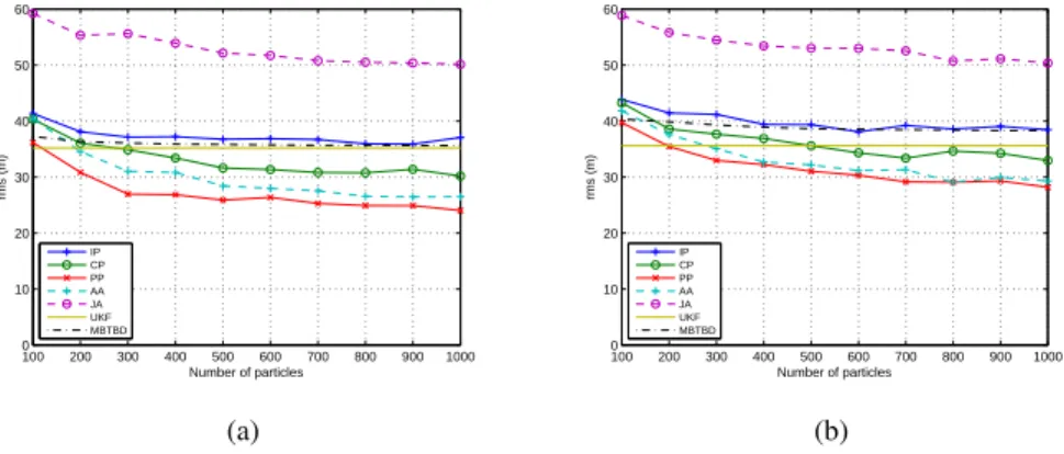
(a). JA performs more poorly because it does not perform subparticle crossover when the targets are far apart. Therefore, this PF acutely suffers from the curse of dimensionality that consists of a drop in performance when the dimension of the state increases [17]. The UKF does not perform properly either. It is better than all the PFs when there are only 100 particles but its performance is far from the performance of PP when the number of particles is high because the measurement model is highly non-linear. Nevertheless, as pointed out in [45], the UKF has much better performance than JA in a multiple target tracking scenario. CP performs better than IP as expected [6] but much worse than PP. This is due to the fact that IP and CP draw subparticles of the targets without taking into account the other targets. This is of crucial importance when we use non-thresholded data and there is a crossing in the targets’ trajectories. Moreover, as AA does not perform subparticle crossover when the targets are in the same cluster, its performance is not as good as PP’s because it is difficult to find particles in which all subparticles are good for representing the multitarget state when the number of particles is low. Nevertheless, when the number of particles increases, the importance of subparticle crossover decreases as it is easier to have particles in which all subparticles are appropriate for the multitarget state and the difference between AA and PP becomes smaller. On the other hand, MBRFS performance is far from PP, AA and CP performances. This was expected as MBRFS using non-thresholded data was developed under the assumption that the targets are far from each other [3]. We should clarify that we have not used the K-means algorithm for partition sorting in the PFs as suggested in [6]. K-means is an enforced method to speed up the removal of the multimodality of the posterior PDF after a target crossing [52] to facilitate target state estimation. Thus, including it would depart from the Bayesian perspective we want to follow in this paper. Nevertheless, we have also implemented it and, for this scenario, its effects are negligible as targets cross with different speeds so there are very few partition swappings [6].
The time-averaged RMS position error using binary data for all the algorithms is shown in Fig. 4 (b). The use of binary data implies a higher error as there is less information available. We can draw the same conclusions about the algorithms as when using non-thresholded data. However, as the number of particles increases, the difference between AA and PP is lower than before. This means that subparticle crossover is not so important with binary sensors. This can be attributed to the severe quantisation of the measurements making it is easier to find full particles that agree with the measurement.
Further insight into the behaviour of the various algorithms can be gained by plotting the RMS position error and the estimated number of targets against time. These plots are shown in Fig. 5 for non-thresholded data using 500 particles for the PFs. We divide the simulation into two intervals to explain the plots:
100 200 300 400 500 600 700 800 900 1000 0
10 20 30 40 50 60
Number of particles
rms (m)
IP CP PP AA JA UKF MBTBD
(a)
100 200 300 400 500 600 700 800 900 1000 0
10 20 30 40 50 60
Number of particles
rms (m)
IP CP PP AA JA UKF MBTBD
(b)
Figure 4 – Time-averaged RMS position error using non-thresholded data (a) and binary data (b). PP method
outperforms the rest of the PFs because it performs subparticle crossover and considers nearby targets.
same performance as they are indeed the same PF when the targets are far from each other. AA has high performance as well because it also uses subparticle crossover when the targets are not in the same cluster. MBRFS also provides good estimates as the targets are not close. On the contrary, JA does not work properly because it does not use subparticle crossover. The UKF does not work properly either because the measurement model is highly nonlinear.
• Second interval: From time step 85 to 130. There are targets in close proximity. PP is the algorithm with the highest performance in RMS error and estimating the number of targets because it takes into account nearby targets and it also performs subparticle crossover. AA and UKF are roughly the algorithms with the second highest performance as they also take into account nearby targets. Conversely, IP and CP performances slump because they do not take into account targets in close proximity to propagate the particles. MBRFS does not perform well either because the targets are close to each other.
20 40 60 80 100 120 0
10 20 30 40 50 60 70 80
time step
rms (m)
IP CP PP AA JA UKF MBTBD
(a)
20 40 60 80 100 120
0 0.5 1 1.5 2 2.5 3 3.5 4 4.5 5
time step
Number of targets
IP CP PP AA JA UKF MBTBD Real
(b)
20 40 60 80 100 120
0 20 40 60 80 100 120
time step
OSPA (m)
IP CP PP AA JA UKF MBTBD
(c)
Figure 5 – RMS position error (a) and estimated number of targets (b) using non-thresholded data per time step
with 500 particles (c) MOSPA position error. Before time step 85, IP, CP, PP, AA and MBRFS have roughly
the same performance because the targets are far from each other. When the targets get closer, PP outperforms
20 40 60 80 100 120 0
10 20 30 40 50 60 70 80 90 100
time step
Number of surviving subparticles (%)
IP CP PP AA JA
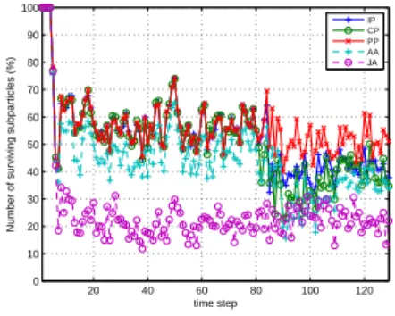
Figure 6 – Number of surviving subparticles using 500 particles. PP has the highest survival rate.
Table VI – Execution times in seconds for 500 particles
IP CP PP AA JA UKF MBRFS
Non-thresholded 32.7 35 34.3 37.4 39.2 0.5 5.5
Binary 29.8 30.5 30.2 30.1 32.1 0.5 5.4
We also show the number of surviving subparticles per time step in Figure 6. We should note that the implemented PFs perform a resampling stage after each time step. Then, the subparticles at time k are based on only some subparticles at timek−1(the surviving subparticles) because the rest have not been selected because of their low weight. The higher the number of surviving particles, the most likely there are particles that represent the posterior well. A survival rate of between 30–80% is generally seen as acceptable [18]. Before time step 85, IP, CP, PP and AA have the same number of surviving subparticles. However, when the targets get closer, PP has the highest number of surviving subparticles and is able to maintain an acceptable survival rate. Before time step 4, all the algorithms have 100% survival rate as no targets have been added yet.
In Table VI, we show the execution times of the algorithms implemented in Matlab with C-MEX subroutines on a Pentium IV with a 2.4-GHz processor. The UKF is the fastest algorithm as it only approximates the first two moments of the posterior. In addition, processing non-thresholded data takes more time than processing binary data as the likelihood is faster to evaluate with binary data, see (17) and (19). For this scenario, computational time increases roughly linearly with the number of sensors and the number of particles.
Table VII – Required number of particles to obtain an RMS position error lower than 25 m
Number of targets
Method 4 8 12 16 20 24 28 32
PP 300 300 300 500 500 800 800 900
MBRFS 8700 8700 8700 8700 8700 8700 8700 8700
IP >10000 >10000 >10000 >10000 >10000 >10000 >10000 >10000
CP 600 8300 >10000 >10000 >10000 >10000 >10000 >10000
AA 400 1600 2800 6200 >10000 >10000 >10000 >10000
two targets. More details of this scenario are given in [9]. For a given error, MBRFS is able to track 32 targets with the same, albeit large, number of particles as with 4 targets because of its nonoverlapping assumption. This suggests that MBRFS would be the most suitable algorithm for tracking large numbers of targets. This conclusion is true only if targets remain well-separated. If several targets move in close proximity then the performance of MBRFS deteriorates, as seen in Figures 4 and 5. On the other hand, the proposed method (PP) provides a favourable trade-off between performance and computational expense. It is not limited to the case of well-separated targets and the required sample size increases by only three times as the number of targets is increased from 4 to 32. The remaining PFs fare much worse.
B. Estimation of the number of targets
Now, we compare our algorithm to the existence grid, whose details can be found in [7], [25], and the MBRFS with regard to the creation and deletion of tracks. The existence grid is a method to construct the importance densities governing target addition q2(·) and removal q3(·) based on partitioning the
surveillance area into cells that form a rectangular grid. The pixelised sensor model is used in this section because the existence grid was designed to deal with this sensor model [7].
The existence grid provides a measure of the chances that a target is located in a cell, denoted as gkj
in cell j at timek [7]. It is updated sequentially according to the measurement, the prior probability of adding a target in a cell α and the prior probability of removing a target β. In our simulations, rather than using the equation of the importance density to remove targets using the existence grid, equation (53) in [7], which permits a target removal probability exceeding one5, we use the following probability
5This happens for instance when there are two targets,gk
1 = 0.99,g2k= 0.001and β= 0.6, thenτ2k= 1.188which is not
0 1000 2000 3000 4000 5000 0
500 1000 1500 2000 2500
x position (m)
y position (m)
1 2
3 4 5
6 7 8
Figure 7 – Trajectories of the targets used to analyse the estimation of the number of targets
of removing target i:
τik=
β·1−gvkk
i
Ptk−1
l=1
1−gk vk
l
(49)
where vk
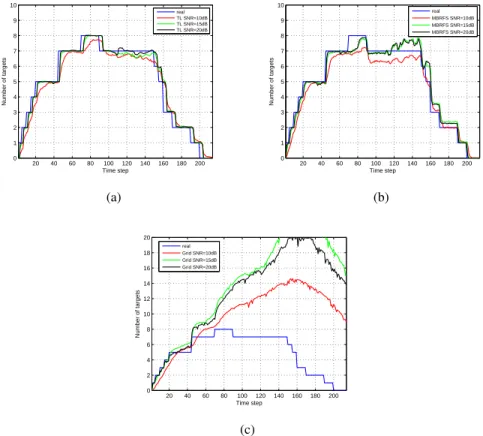
i denotes the cell occupied by the ith target at timek. In (49), the division of the denominator by the number of targets, which appears in (53) of [7], has been removed. The resulting target removal probability is at most β. The existence grid does not take into account targets’ dynamics because the equation that models them, equation (11), is not used and, besides, it does not account for the possibility that a target might move to another cell. Then, the performance of the existence grid is much lower than the performance of our two-layer PF, especially when the targets move fast. In this case, performance mainly refers to the ability of the filter to create and delete tracks in a timely manner.
The scenario we use is shown in Fig. 7. The prior parameters are the same as in the previous example, see Table V, but withσu= 10 m/s3/2. The parameters of the two-layer PF areNb = 3,ηb=e7,Nd= 5,
ηd=e−2 for the two-layer PF. The parameters for the existence grid areα= 2·10−15 andβ = 0.9. The surveillance area is a square whose side is 5000 m long. This region is divided into 50 × 50 cells and each cell scans a 100 m ×100 m area.