Edge Detection by Adaptive Splitting II. The Three-Dimensional Case

Edge Detection by Adaptive Splitting II.

The Three-Dimensional Case

Bernardo Lianas • Sagrario Lantaron

Abstract In Lianas and Lantaron, J. Sci. Comput. 46, 485-518 (2011) we proposed an al-gorithm (EDAS-<i) to approximate the jump discontinuity set of functions defined on subsets of Rd. This procedure is based on adaptive splitting of the domain of the function guided by the value of an average integral. The above study was limited to the ID and 2D versions of the algorithm. In this paper we address the three-dimensional problem. We prove an integral inequality (in the case d = 3) which constitutes the basis of EDAS-3. We have performed detailed computational experiments demonstrating effective edge detection in 3D function models with different interface topologies. EDAS-1 and EDAS-2 appealing properties are extensible to the 3D case.

Keywords 3D edge detection • Jump discontinuity set • Adaptive splitting • Implicit smoothing • 3D high-resolution imagery

1 Introduction

1.1 The Edge Detection Problem

The detection of objects in volumetric data sets is a challenging problem due to the size of the data and the variability of the features of interest. Depending on the concrete analysis task the accurate detection of edges can be very important. For example, the estimation of geometric and differential properties of reconstructed object boundaries such as volume, curvature or even higher order properties requires particularly accurate edge localization algorithms. Due to its technological importance, many procedures have been proposed to determine 3D edges (interfaces). Below, we give a (non-exhaustive) classification:

- Direct Methods. The aim of these methods is to determine the edges of a determined function.

- ID edge detection methods. These procedures can be extended to detect the size and position of discontinuities of a multi-dimensional function by holding all but one di-mension fixed and determining the edges as a function of the fixed coordinates. A prac-tical application of this method is described in [1, 5]. The concentration edge detection algorithm [14] and the Gegenbauer reconstruction method [15] are combined to pre-process the data.

- Spatial difference filters [37]. These methods are used for detecting edges in digital 3D-images. An image is a discretely defined function. Its domain is a set of nodes in a regular grid. The local function of this type of filters contains the calculation of the difference between density values of an input image. Most 3D filters can be synthesized from 2D filters. The 3D difference filters were first reported in [22]. In some cases the computation cost of these methods may become excessive.

- Polynomial fitting method [3, 4]. This method is based on a local polynomial annihila-tion property on a set of irregularly distributed points in a bounded domain of Rd. - Deformable models. These methods consider a geometric object surrounding the

in-terest area (active contour) depending on several parameters. They define an energy functional which consists of the sum of an internal and an external energy. When the functional in minimized, the internal energy constraints the shape of the active contour and the external energy locates the contour in desired image features.

Deformable models can be broadly classified into explicit or implicit models. • Explicit methods (snakes) were introduced by Kass et al. [20] and generalized to 3D

by Terzopoulos et al. [36]. They represent the object by means of meshes (curves, surfaces or solids) which shape evolves in the minimization of energy process. How-ever, since the model topology is created before the deformations, explicit models are not generally able to segment complex shapes with genus higher than 0. In or-der to overcome this limitation, several methods have been developed in past years: T-snakes [26], active volume methods [7, 32], etc.

• Implicit methods (level set formulation) In the late 1990s, Sethian et al. [31] pro-posed a new framework called level set. The basic idea was to embed the contour evolution into iso-value curves of a function with higher dimensionality. Such func-tions were called level set funcfunc-tions. This kind of representation of contours and surfaces provides topological flexibility in the segmentation process so that the topo-logical changes are automatically handled. However, it makes difficult the user in-teraction and increases the computational cost. A recent formulation of this method is given in [27].

Deformable models present some inconveniences such as sensibility to the initial con-tours, stopping at local minima of the energy, slowness, and computational cost. - Indirect Methods. The aim of these methods is to divide the domain of the function into

procedures include region-based algorithms [21, 42] and registration based segmentation [35].

1.2 An Adaptive Splitting Algorithm for 3D Edge Detection

Adaptive splitting procedures have been used in approximation theory (see, for example [25], and the references therein). Adaptive meshing methods for edge detection have been studied mainly in the context of image processing (discretely defined functions). In image multiscale analysis, adaptive (nonuniform) grids for the finite element method applied to the Perona-Malik equation [29] with the modification suggested in [11] were studied in [6] (3D case). In image segmentation and representation (see [23] for a recent account), many algorithms are based on adaptive approaches. Most adaptive methods produce an image segmentation using a variant of the split and merge method [18, 41].

An adaptive splitting approximation algorithm was proposed in [25]. In [24] it was proved (for d = 1 and d = 2) that the average integral used in its splitting criterion is an effective jump detector. These results imply that the algorithm is divergent for functions with jump discontinuities, but they allow us to modify it to obtain an efficient edge detection method.

In this paper we extend the above results to the three-dimensional case. We study the capability of EDAS-3 to detect 3D edges. The parameters of the original approximation algorithm have a new additional meaning. The local error gives the detection threshold. The stopping criterion gives the precision of the obtained jump points. We introduce new parameters to optimize the search for jumps and the numerical computations.

EDAS-3 is an algorithm to detect jump discontinuities of functions defined by data in the physical space. The domain of the function is supposed to be the difference of a convex set and a set of Lebesgue measure zero (continuously defined functions). Its output consists of an approximation of the jump discontinuity set of the function (see Sect. 2). It is based on an integral inequality fulfilled by the sets containing a jump discontinuity.

The algorithm builds a piecewise affine function which provides a rough approximation of / away from the discontinuities. In the neighbourhood of an edge, this function is a good approximant. The integrals whose evaluation is necessary to obtain the piecewise affine function are computed by numerical methods which are exact for polynomials of a certain degree. This provides an "implicit smoothing" of the target function, that accelerates the convergence away from the discontinuities and makes the algorithm robust in the presence of noise.

The choice of the local error is guided by the magnitude of the searched jumps rather than by the degree of approximation away from the discontinuities. This allows to obtain good results with a poor approximation (homogeneity property) when the magnitude of the jumps is large enough.

The search procedure of EDAS-3 and its flexible way of representing interfaces allow to handle automatically topological changes. In addition, EDAS-3 overcomes some of the limitations of deformable models:

Initial conditions (contours), are not necessary.

It is not a variational approach. This avoids the problem of stopping at local minima of the energy.

It does not need to use complicated data structures. The implicit smoothing implies a relatively fast processing.

Finally, in the case of complex problems, we can partition the domain and apply EDAS-3 independently to each subdomain. This allows parallel processing.

This paper is organized as follows. Section 2 gives some mathematical preliminary re-sults and states the main result of the article. In Sect. 3 we recall the EDAS-<i algorithm and detail its implementation for d = 3. Section 4 presents 3D computational experiments with synthetic and real models. Section 5 provides some concluding remarks. The paper is closed with an Appendix containing the proof of Theorem 1.

2 Mathematical Preliminaries

Let R C W be a compact <i-interval. We say that a function g : R -> R is quasi-continuous if the set of points where g is not continuous has zero Lebesgue measure.

Consider a finite collection {C,}"=1 of connected sets with pairwise disjoint nonempty interiors such that

n

Let {/,- : i = 1 , . . . , n} be a set of continuous functions on R. Define the function / ( x ) = /Kx) if X G Q ,

where C denotes the interior of C. We say that / is a general piecewise continuous function. If Q , i = 1 , . . . , n, are closed and convex sets, we say that / is a piecewise continuous function. Since the boundary of a convex set has zero Lebesgue measure, all piecewise

continuous functions are quasi-continuous.

In the above definition, if the functions f, i = 1 , . . . , n, are constant, we say that / is a general piecewise constant function and a piecewise constant function, respectively.

Let / be a general piecewise continuous function and let r,- be the boundary of Q , i = 1 , . . . , n. Define T = U"= 1 r,-. Let x e T, then for some m < n, x e i y , j = 1 , . . . , m, where ij e {1, 2 , . . . , « } . Define

A= max {/;,(x)}, and B = min {/;,(x)}.

j=l,...,m j=l,...,m

discontinuity set. The set of points in FJ with magnitude of jump greater than I is denoted

by Ff. The set of points in FJ with magnitude of jump greater than I and lower than u is

denoted by TJlu. Our aim is to obtain a good approximation of these sets for a given function.

We use the term interface as an abbreviation for jump discontinuity set.

The d-simplex T generated by the set of affinely independent vectors {vo, v i , . . . , v^}, denoted by (v0, V i , . . . , vd), is defined to be the convex hull of the vectors v0, V i , . . . , vd. We denote by \T\ the diameter of a <i-simplex T.

Consider a function / : T C W -> R. We denote by LTf, the unique affine map such

that

LTf(vj) = f(vj), j=0,l,..-,d.

In this section we study the average integral

A W ) :

f

T

\f(x)-L

f(x)\dx

v(T)

where v(T) denotes the Lebesgue measure of T.

As we prove below, the behavior of AIT(f) depends on the continuity or lack of

conti-nuity of / on T. This fact lays the foundation for the algorithm proposed in the next section. The comportment of AIT(f) when / is continuous is given by the following result.

Proposition 1 ([13]) Let X c M ^ t e compact and let f : S -> R be continuous. Then given e > 0, there exists S > 0 such that

| / ( x ) - L

/ ( x ) | < e

for all xeT, where T is a d-simplex contained into S with \T\ < 8.

Corollary 1 Let S C Rd be compact and let f : S -> R be continuous. Then given e > 0, we have that AIT(f) < e for any small enough d-simplex T C S.

If / is smooth the above result can be sharpened, see [24].

From the above result, we can conclude, in the case of continuous functions, that A / r ( / ) —>• 0 as |T| approaches zero. We study below the case in that / presents jump discontinuities on T, when d = 3.

From now on, we limit ourselves to the case where f(x) is a function of Heaviside type. This suffices to study image processing applications and functions with smooth T J.

Consider the Heaviside function

fo, i f x < 0 , [ l , i f x > 0 . We have

Theorem 1 Let h : R3 —»• R be the function defined by h(x) = JH{ax\ + bx2 + ex?, + d),

arbitrary tetrahedron in R3 such that r C\t ^0. Then

1J jT\h(x)-LTh(x)\dx 3 /

<" — — - — < — , (1) 32 ~ v(T) ~ 4

where v(T) is the volume ofT.

The proof of this theorem is given in the Appendix.

3 Edge Detection by Adaptive Splitting Algorithm

3.1 Statement of the Algorithm

We state the algorithm in the <i-dimensional case. Consider the <i-interval R = [a, b], where a,b eW. We can find n (closed) simplices Tt such that

t

n fj = 0, i ^ i,

n

{jT

i = i

(for example, see [9, 28]). We call P = {Tt}"=1 a partition of R. The set of partitions of R is

denoted by V(R). Given a <i-simplex T we denote by V(T) the set of its vertices.

The proposed algorithm builds a partition P e V(R) and the associated piecewise affine approximant L (x) defined by

L(x) = LTf(x) ifxeTcP.

The average integral

A W )

f

\f(x)-L

f(x)\dx

v(T) can be considered as the local error of the approximant L.

Given a function / : R —»• R and an initial partition Pi of R, denote by E\ the maximum local error of the approximant L. In the cases where Theorem 1 can be applied, E\ also provides a detection threshold, because the algorithm will detect the jumps with magnitude greater than 3 2 £ i / 7 . Denote by E2 the approximation error of the points in FJ. Let £4 be a

positive real parameter.

If (AIT(f) < Ei ov \T\ < E2) and \T\ < £4 we call T a good simplex, otherwise T is

called bad.

We call EA, exploration parameter (in difficult problems, it is necessary to make £4 small. This is due to the fact that an inaccurate numerical evaluation of AIT(f) can eliminate

Edge Detection by Adaptive Splitting Algorithm (EDAS-d)

Step 1. The good simplices in the initial partition Pi axe put into the set Gi and the bad simplices are put into the set B\.

Step 2. At each step j we have a set of good simplices Gj and a set of bad simplices Bj. Divide each bad simplex into two simplices, by splitting its largest edge. Test whether these children are good or bad to obtain the sets Gj+i and Bj+i.

Step 3. The algorithm stops if Bj = 0. Then G = Gj is the searched partition. If the stopping criterion is not satisfied, go to Step 2.

Step 4. Obtain the following subset of G

ATE ={TeG: AIT(f) > Ex and j " = max {/(«,-)} - min {/(«,-)} > £3}.

3 VieVfT) v^V(T)

where £3 is the minimum magnitude of jump reported. £2 is also a stopping criterion. The convergence of this algorithm is guaranteed by the definition of good simplex. ATJE is a

set of simplices containing points of TJE . This constitutes an approximation of TJE . In the

cases considered by Theorem 1, we have that ATJE D TJE . In Sect. 4, instead of describing

AY I, we have considered the set of barycenters of T e ATJE to better visualize the result.

3.2 Practical Implementation of EDAS-3

In practice we have implemented the above algorithm using a tree whose leaves correspond to good simplices. Tree construction follows a technique similar to that detailed in [25]. The integrals fT | / ( x ) — LTf(x)\dx have been computed using the Grundmann and Moller's

formula [17].

We have considered a positive real parameter £5 (adaptivity of cubature formulas param-eter). This factor allows to apply higher degree cubature formulas in large regions and low degree cubature formulas in small regions. In this way the computational cost is optimized. The adaptive cubature procedure is described below.

- If \T\ < £5, the computations have been done using the Grundmann and Moller's rules of degree p = 5,7,9, 11, 13, and 15 with d = 3. Due to the lack of error estimates for the Grundmann and Moller's rules, we have followed the usual practice of comparing succes-sive values of the integral corresponding to an increasing number of points and taking the value obtained when the sequence becomes stationary. We denote by AIT(f) the value

of AIT(f) computed by the cubature rule of degree p. The pseudocode is described by

the following statements. Set p = 5;

Compute AIT(f) and AIT(f);

while (\AIPT(f) - AIPT+2(f)\ > E^W && p < 13) {

if (\AIPT(f) - AIPT+\f)\ < Er/10) Ahif) = AIPT+\f);

else A /r( / ) = 106;

- If | r | > £5, the computations have been done using the Grundmann and Moller's rules of degree p = 13 and 15 with d = 3. The corresponding pseudocode is listed below.

if (JA/J? (/) "

< Ei/10) Ah(f) = Ti\

-else A /r( / ) = 106;

To sum up, the algorithm requires the following positive real parameters - E\: Maximum local error of the approximant L and detection threshold. - E2: Approximation error of the points in FJ and stopping criterion.

- £3: Minimum magnitude of jump reported. - £4: Exploration parameter.

- £5: Adaptivity of cubature formulas parameter. 3.3 Theoretical Foundation of EDAS-3

Results in Sect. 2 guarantee the convergence away from the discontinuities and the suitable local behavior of EDAS-3. We can consider three cases:

- Piecewise constant functions whose FJ consists of a set of planes. Theorem 1 can be

ap-plied to most tetrahedra in a partition. 3D images are an example of this type of functions (Sect. 4.4).

- General piecewise constant functions with curved T /. If the interface is smooth enough, then Theorem 1 is approximately valid when the tetrahedra become very small (Sects. 4.1, 4.2 and 4.3).

- General piecewise continuous functions. In this case, Theorem 1 is not directly applicable. In spite of this, EDAS-3 has given good results in some particular cases (Sect. 4.5).

4 Computational Experiments

The experimental environment has been the following: • CPU QuadCore Intel Core 2 Quad 6700, 2666 MHz. • RAM 4GB.

• Running software Microsoft Visual C.

We have considered different functions / : R -> R, where R is a cube in R3. Each face of R has been divided into four triangles by means of its diagonals. The vertices of these triangles and the center of the cube yield a division of R into 24 disjoint tetrahedra. This resulting set has been used as the initial partition Pi of EDAS-3.

Given a function and the parameters {£•, i = 1,5}, we use the following point-based representation of the approximated jump discontinuity set to show the results

P AFE3 = {x G R3 : x is the barycenter of some T e ATJE^}.

Let I, u be real numbers such that I < u. Define

Table 1 Dependence of E\ on /

E2 E3 E4 E5 TNT TNJT CPU (s)

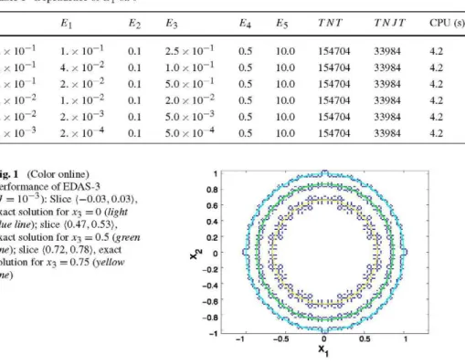
10" 10" 10" 10" 10" 10" 10" 10" 10" 10" 10" 10" 0.1 0.1 0.1 0.1 0.1 0.1 2.5; 1.0; 5.0; 2.0; 5.0; 5.0; 10" 10" 10" 10" 10" 10" 0.5 0.5 0.5 0.5 0.5 0.5 10.0 10.0 10.0 10.0 10.0 10.0 154704 154704 154704 154704 154704 154704 33984 33984 33984 33984 33984 33984 4.2 4.2 4.2 4.2 4.2 4.2

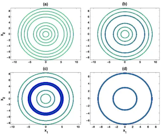
Fig. 1 (Color online) Performance of EDAS-3 (/ = 10~3): Slice (-0.03,0.03), exact solution for xj = 0 (light

blue line); slice (0.47,0.53),

exact solution for xj = 0.5 (green

line); slice (0.72, 0.78), exact

solution for xj = 0.75 (yellow

line)

The slice (I, u) is defined as the projection of [\l, u\] on the plane %\ — x2. All the accom-panying graphs show (I, u) for different values of I and u. We have represented them as a cloud of dark blue points. The intersections of FJ and planes perpendicular to the x3-axis

(exact solutions) have been drawn as continuous colored lines.

Numerical data tables include the total number of tetrahedra generated by EDAS-3 (TNT), and the number of tetrahedra containing jump points inside them (TNJT).

In all experiments, CPU time is expressed in seconds and denoted by CPU (s). 4.1 General Properties of EDAS-3

In this section we study experimentally the following general properties of EDAS-3: - Dependence of the parameter E\ on the magnitude of the jump ( / ) .

- Dependence of the precision on the parameter E2.

- Robustness against continuous and discontinuous random perturbations.

To study the dependence of the parameter E\ on / , we have considered the general piecewise constant function with spherical interface

/ l ( X l , X2, X3) :

1, if (xi,X2, X3) G S i ,

1 + / , if ( x ! , X 2 , x3) G R — Bi,

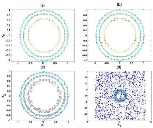
Table 2 Dependence of the precision on the parameter E2 / 0.5 0.5 0.5 El 0.1 0.1 0.1 E2 0.10 0.05 0.01 £3 0.25 0.25 0.25 £4 0.5 0.5 0.5 £5 10.0 10.0 10.0 TNT 154704 325824 5782896 TNJT 33984 134592 3269856 CPU (s) 4.2 12.3 272.2 (a) 1 — 0.8 0.6 0.4 0.2 0 -0.2 -0.4 -0.6 -0.8 1 -0.8 0.6 0.4 0.2 J> 0 -0.2 -0.4 -0.6 -0.8 -1

/?

I f :/

:

|

;

-1 -0.5 (b)

'- L CH L"

0

$N\

:

\

\ \

f i t

0.5 1

Fig.2 Precision versus E2-Slice (—0.01,0.01), exact solution for X3 = 0 (light blue line); slice (0.49,0.51), exact solution for X3 = 0.5 (green line); slice (0.74, 0.76), exact solution for X3 = 0.75 (yellow line): (a)

E2 = 0.1, (b) E2 = 0.05, (c) E2 = 0.01

Since 7/32 ~ 0.22, Table 1 shows a good agreement between the experimental results and those predicted by Theorem 1.

To find the relationship between the precision and the parameter E2, we have considered

the function f\ with / = 0.5 and E\ = 1 0- 1. We have varied E2- The results are given in

Table 2. Figure 2 shows how the precision of EDAS-3 increases as E2 decreases.

To study the effect of continuous noise on the performance of EDAS-3, we have used the continuously perturbed function

f[(xi,x2,x3):

1 + a sin(100(x! + x2 + X3)), if (xi,x2,x3) e B\,

Table 3 Performance of EDAS-3 on the continuously perturbed function

co

0.00 0.05 0.10

El

0.05 0.05 0.05

E2

0.1 0.1 0.1

E3

0.25 0.20 0.20

E4

0.5 0.5 0.5

E5

10.0 10.0 10.0

TNT

155616 11343840 24149916

TNJT

34896 33906 34326

CPU (s)

4.5 1042.9 2543.3

(a) (b)

Fig. 3 Performance of EDAS-3 on the perturbed f\ (the endpoints of the slices are the same as those in Fig. 2): (a) ff, El = 0.05, co = 0, (b) ff, El = 0.05, co = 0.1, (c) f[p, El = 0.1, co = 0.4, (d) f[p, £ 1 = 0.1, co = 0.5

The results obtained with several values of co are reported in Table 3. Figure 3(b) shows that a noise with magnitude 20 percent of the jump, does not change the result obtained with a = 0; see Fig. 3(a).

Tables 2 and 3 show an increase in the number of tetrahedra that is due to different reasons. In Table 2 we increase the precision of EDAS-3 by decreasing the value of the parameter E2- As a result, a large increase of tetrahedra arises around the discontinuity

Table 4 Performance of EDAS-3 on the randomly perturbed function Q) 0.10 0.20 0.30 0.40 0.50 El 0.1 0.1 0.1 0.1 0.1 E2 0.1 0.1 0.1 0.1 0.1 E3 0.45 0.45 0.45 0.45 0.45 E4 0.5 0.5 0.5 0.5 0.5 E5 10.0 10.0 10.0 10.0 10.0 TNT 661030 2538203 5946536 9866541 13071176 TNJT 27237 26220 26221 26839 485582 CPU (s) 95.1 403.7 976.4 1652.9 2220.4

To study the effect of discontinuous random noise on the performance of EDAS-3, we have used the randomly perturbed function f[p = fi + a> rp, where

rp(x1,x2,xi) = r(i1,i2,ii), ij = 0, . . . , 7 9 ,

_ f floor(Aj), if Aj^SO,

lj=[79, if A; = 80,

Aj = 10-(4+ Xj), j = 1,2,3.

r is a random matrix with 512000 entries between 0 and 1 defined in MATLAB by r = ra«<i[80][80][80]. floor (x) is a MATLAB function that gives the largest integer not greater than x. The resulting function rp is a piecewise constant random function.

The results obtained by EDAS-3 for several values of the parameter a are given in Ta-ble 4. If a is less than 0.5, thresholding ( £3 = 0.45) avoids the detection of noise jumps; see Fig. 3(c). If a = 0.5 the magnitude of many noise jumps equals 0.5 (jump of true edge points) and the algorithm detects them; see Fig. 3(d). Since by Theorem 1, the jumps with magnitude less than 4 £1/ 3 are not detected, we can state that implicit smoothing, threshold-ing and the value of the parameter E\ are the procedures of EDAS-3 to avoid noise effects. 4.2 General Piecewise Constant Function with Tubular Tree-like Interface

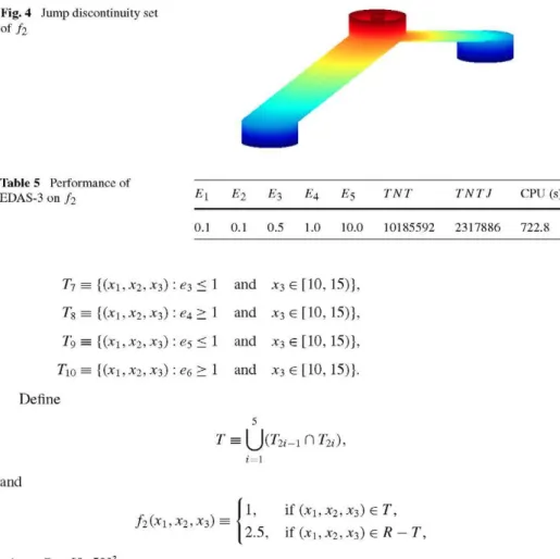
Blood vessels and airways of the human body form dense tubular tree-like structures. The segmentation of these structures in volumetric datasets is of vital interest for many medical applications [8, 38]. In the following example we define a function with a multiply connected interface which models a vascular/bronchial tube. We need some previous definitions

e, = (x! - 25)2/16 + (x2 - 25)2/4, e2 = (Xl - 25)2 + (x2 - 25)2,

e3 = (x! - 10)2/16 + (x2 - 10)2/4, e4 = (xx - 10)2 + (x2 - 10)2,

e5 = (x! - 40)2/16 + (x2 - 40)2/4, e6 = (Xl - 40)2 + (x2 - 40)2,

hx = (x3 - 15)/10, / !2= ( 2 5 - x3) / 1 0 . 7\ = {(x!,x2, x3) : e\ < 1 and x3 e [25, 30]}, T2 = {(x!,x2, x3) : e2 > 1 and x3 e [25, 30]},

r3 = {(x!,x2, x3) : h\e\ + h2e3 < 1 and x3 e [15, 25)},

TA = {(xi,x2, x3) : h\e2 + h2e4 > 1 and X3G [ 1 5 , 2 5 ) } , Ts = {(xl7x2, x3) : h\e\ + h2es < 1 and x3e [ 1 5 , 2 5 ) } ,

Fig. 4 Jump discontinuity set of/2

Table 5 Performance of

EDAS-3 on f2 El

0.1

E2

0.1

E3

0.5

E4

1.0 £5

10.0

TNT

10185592

TNTJ

2317886

CPU (s)

722.8

r

:

{(xi,X2, X3) : e3 < 1 and X3G[10, 15)},

{(x!,x2, x3) : e4 > 1 and X3G [ 1 0 , 15)},

{(x!,x2, x3) : es < 1 and X3G [ 1 0 , 15)},

{(xi,X2, X3) : ee > 1 and X3 € [10, 15)}. Define

r ^ Q c r ^ i n 7-2,-),

and

f2(xUX2,X3) :

1, if (xi, X2, X3) G r ,

2.5, if (xi, x2, x3) G i? — r , where fl = [0,50]3.

Figure 4 shows the interface (FJ) of /2. The results obtained are reported in Table 5. Figure 5 shows a comparison between the slices of the cloud of points generated by EDAS-3 and the intersections of the interface with planes perpendicular to the xEDAS-3-axis.

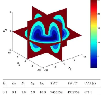
4.3 General Piecewise Constant Function with Disconnected Interface

This experiment shows the capability of EDAS-3 for dealing with functions having inter-faces with a complex topological structure.

In this case R = [—10, 10]3. The equation of a torus with axis X3, inner radius r, and rf. Let r„

outer radius r0 is given by (r0

(5 — Jx\ + x | )2 + x\. Define

X j - p X2) ~T~ x ^ 5 and D(x\, x2, x3)

/ 3 ( X ! , X 2 , X3) :

10 15 20 25 30 35 40 45 1

10 15 20 25 30 35 40 45

1

Fig. 5 (Color online) Performance of EDAS-3 on fx- The exact solutions corresponding to xj = (I + «)/2 for each slice (/, u) are the continuous green lines: (a) slice (29.95, 30.05), (b) slice (26.95, 27.05), (c) slice (24.75,24.80) (the exact solution is the part of the green lines contained in the cloud of points), (d) slice (16.95,17.05), (e) slice (11.95,12.05), (f) slice (9.95, 10.05)

Figure 6 shows the graph of /3. The results obtained with EDAS-3 are reported in Table 6.

Figure 7 shows a comparison between the slices of the cloud of points generated by EDAS-3

Fig. 6 Function fj

xf o

I

1:

•1i

10

J

Table 6 Performance of

EDAS-3 on /3 El

0.1

E2

0.1 £3

1.0 £4

2.0 £5

10.0

TNT

9455552 TNJT

4972752

CPU (s)

671.1

4.4 Performance on Real 3D Images and Comparison with other Methods

In this section we study the performance of EDAS-3 on 3D images. These images are dis-crete functions given by 3D-arrays. They can be extended to piecewise constant functions. The interface of these extended functions consists of a set of planes. Therefore, Theorem 1 can be applied to most tetrahedra in a partition. In the experiments we have used a 3D image obtained by linear interpolation (At + (1 — t)B) of two CT section images (A and B) of a real brain (Radiology, Uppsala University Hospital) [19]; see Fig. 8. Interpolation from serial cross sections is a customary practice when the sections are not closely spaced [16]. In this way the appearence of the embedded 3D object is recaptured.

The test 3D image exhibits a complex structure containing several three dimensional ob-jects. In complex problems, it may be difficult to use deformable model algorithms. There-fore, we have compared EDAS-3 with 3D difference filters (Sobel, Prewitt) which are suit-able for arbitrary (unstructured) images. In the experiments with the 3D-Sobel method, the following mask to obtain the partial derivative of the image intensity with respect to the variable x\, was adopted:

MX(:,:,l) = [-20 2; - 3 0 3 ; - 2 0 2 ] , AfX(:,:,2) = [-3 0 3; - 6 0 6; - 3 0 3], AfX(:,:,3) = [ - 2 0 2; - 3 0 3 ; - 2 0 2 ] . The corresponding mask used for the 3D-Prewitt method is:

(a) (b)

Fig. 7 Performance of EDAS-3 on fj. The exact solutions corresponding to xj = (I + «)/2 for each slice (/,«> are the continuous green lines: (a) slice (—0.05,0.05), (b) slice (1.45, 1.55), (c) slice (1.95,2.05), (d) slice (3.45,3.55)

We have used the MATLAB notation for matrices. The masks for the derivatives with respect to x2 and x3 can be obtained from the above ones [37, 39].

From each original 2D-image (A and B) of size 5 1 2 x 5 1 2 we have obtained two images of size 256 x 256 and 128 x 128 using the function imresize of MATLAB. The x3 axis has been divided into h intervals. The value of the image on the x3-interval [k, k + 1], k = 0 , . . . , h — 1 has been (1 — (k/(h — 1))A + (k/(h — Y))B. In this way we have generated 3D images with different resolution.

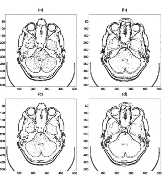
3D-Sobel and 3D-Prewitt algorithms have been programmed in MATLAB and their re-sults are reported in Tables 7 and 8 respectively. Figure 9 shows the performance of these algorithms.

The results obtained by EDAS-3 are reported in Table 9. Figures 10(a) and 10(b) show its performance on the 3D image of size 5 1 2 x 5 1 2 x 2 1 .

We have applied EDAS-2 to the 2D images shown in Figs. 8(c) and 8(d). The results are reported in Table 10. Figures 10(c) and 10(d) show its performance on these images.

Since difference filters need to consider all the voxels, their time behavior is 0(nmh). This fact is confirmed by the experimental results. Therefore, difference filters are not suit-able for high resolution images.

(a)

Fig. 8 3D image of size 512 x512 x 21 obtained by linear interpolation of two CT sections of a real brain. (a) A (real image), (b) B (real image), (c) Interpolated image (t = 0.9), (d) Interpolated image (t = 0.5)

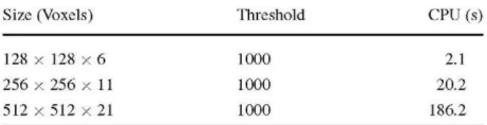
Table 7 Performance of 3D-Sobel on 3D images with different resolution

Table 8 Performance of 3D-Prewitt on 3D images with different resolution

Size (Voxels)

128 x 128 x 6 256 x 256 x 11 512 x 512 x 2 1

Size (Voxels)

128 x 128 x 6 256 x 256 x 11 512 x 512 x 2 1

Threshold

1000 1000 1000

Threshold

400 400 400

CPU (s)

2.1 20.2 186.2

CPU (s)

Table 9 Performance of EDAS-3 on 3D images with different resolution

Size (Voxels)

128 x 128 x 6 256 x 256 x 11 512 x 512 x 2 1

El

0.1 0.1 0.1

E2

0.5 1 2

E3

55 45 30

E4

32 32 32

E5

10 10 10

TNT

18992772 24746155 25235117

TNJT

3569601 4835039 6763826

CPU (s)

3939.3 7349.6 14081.3

(a) (b)

100 200 300 400 500 100 200 300 400 500

(c) (d)

100 200 300 400 500 100 200 300 400 500

Fig. 9 Performance of 3D-Sobel and 3D-Prewitt methods on the image of size 512 x 512 x 21: (a) Sobel

(t = 0.9), (b) Sobel (t = 0.5), (c) Prewitt (t = 0.9), (d) Prewitt (t = 0.5)

considered the relative error (E2/(n + m + h)) constant, but this suffices to get better results as the resolution of the image increases, for example, compare Fig. 11 obtained from the image of size 128 x 128 x 6 with Fig. 10(b). EDAS-3 can handle large size data sets. In fact, the examples studied in other sections of this paper have infinite resolution.

Table 10 Performance of EDAS-2 on images of size 512 x 512

Image

0.9 A + 0.1 B 0.5 A + 0.5 B

El

0.1 0.1

E2

2 2

E3

36 36

E4

10 10

E5

10 10

TNT

102587 102773

TNJT

24558 25399

CPU (s)

12.2 12.3

(a) (b)

(c) (d)

100 200 300 400 500 100 200 300 400 500

Fig. 10 Performance of EDAS-3 on the image of size 512 x 512 x 21: (a) slice (2.3,2.7), (b) slice (10.3, 10.7). Performance of EDAS-2 on 2D images of size 512 x 512: (c) t = 0.9, (d) t = 0.5

Fig. 11 Performance of EDAS-3

on the 128 x 128 x 6 image: slice (2.95, 3.05)

Fig. 12 Function /4 (x \, x2, 0)

The technique of finding edges in different 2D sections of a 3D image is fast and efficient. The results for EDAS-3 are reported in Table 10; see Figs. 10(c) and 10(d). It can be used for medical diagnosis, but if we are interested in a description of the 3D structure we need to use additional reconstruction algorithms.

4.5 General Piecewise Continuous Function

In the case of general piecewise continuous functions which are not piecewise constant, Theorem 1 is not directly applicable. In spite of this fact, EDAS-3 can be applied to solve some of these problems as we see below. Define

f4(xi,x2,x3) =

2 + 0.1 (JCI + x2 + x3) + 3sin(4xi), if (xi,x2,x3) e R — B4,

1 4 + 0.1(JCI + x2) + 2cos(3x2), if (JCI,JC2,JC3) e B4 - E,

27, if (xi,X2,xi) e E,

where R = [—10, 10]3, B4 = {(xi,x2,X3) : x\ + x\ + x\ < 25}, and E = {(xi,x2,X3) :

x\/9 + xf/4 + x | / 4 < 1}. Figure 12 shows the intersection of the graph of f4 with the

plane x3 = 0.

Table 11 Performance of

EDAS-3 on f4 El

0.1

E2

0.1

E3

5.0

E4

1.0 £5

2.0

TNT

9474706

TNJT

1073228

CPU (s)

340.8

Fig. 13 (Color online) Performance of EDAS-3 on f4:

Slice (-0.05, 0.05), exact solution for X3 = 0 (light blue

line); slice (1.45, 1.55), exact

solution for X3 = 1.5 (green

line); slice (2.95, 3.05), exact

solution for X3 = 3 (yellow line)

5 Concluding Remarks

In this paper we study the case d = 3 of the algorithm EDAS-<i. EDAS-3 can approximate the jump discontinuity set of functions defined almost everywhere on convex subsets of R3. The method is based on adaptive splitting of the domain of the function guided by the value of an average integral. The numerical computation of these integrals introduces an "implicit smoothing" that allows a fast convergence away from the jump points. The algorithm needs to specify five parameters which have an intuitive meaning. They can be easily fixed in most problems. While difference filters and deformable models approximate the jump discontinuity set by a set of points and a set of surfaces respectively, EDAS-3 provides a triangulated 3D set that contains the jump discontinuity set. The accuracy of this approximation is fixed beforehand. This is a basic difference with other methods. The output of EDAS-3 does not require reconstruction algorithms and can be used directly as a 3D model.

EDAS-3 allows to handle automatically interfaces with complex topological structure. Initial conditions are not necessary. Since it is not a variational approach, it does not present the problem of stopping at local minima of an energy. In the case of difficult problems we can partition the domain and apply EDAS-3 independently to each subdomain (parallel processing).

We have studied from a theoretical and computational point of view the case d = 3. From the experiments, we can draw the following conclusions about EDAS-3:

It provides a precise determination of the jump points.

The resulting piecewise affine function L does not show oscillatory behavior near the jump points. This makes possible to obtain accurate values of the magnitude of the jumps.

As a consequence, we can obtain stratified edges (Tf, Tfu) in a straightforward manner. In

the case of images, this fact is important because stratified edges correspond to "individual objects" in a scene.

It gives good results for general piecewise continuous functions (not necessarily piece-wise constant).

The CPU-time of EDAS-3 depends on the complexity of the 3D image and on the pre-cision required. In the experiments performed on real images the order of magnitude of the CPU time has been similar to that reported by active volume algorithms.

Some caution is necessary when we apply EDAS-3:

The approximate method of evaluation of integrals can lead to the oversight of some jump points. This can be avoided by decreasing the exploration parameter £4 or by modifying the adaptive procedure to compute integrals.

If the interface presents acute dihedral angles, Theorem 1 may not be applicable to tetra-hedra intersecting the edges of such angles. This part of FJ might be erroneously

approxi-mated.

To sum up, we can state that EDAS-3 is a general procedure to approximate the jump discontinuity set of functions defined on R3. EDAS-3 can be applied to 3D medical im-ages (MRI, CT, etc). This method is specially suitable for dealing with high-resolution 3D images.

Acknowledgement We would like to thank the anonymous reviewers for their careful reading of our manuscript and the insightful comments they provided.

Appendix

In this section we give a proof of Theorem 1. Let a = (a\, a2,... ad), where at e Z+ U

{0}, i = l,...,d. Define

hf = \ dxi I dx2...l f(xux2,...,xd)dxd,

Jo Jo Jo xa = x = (xi, ...,xd)^ x"1 . ..xa/.

Lemma 1 ([17])

Idxa = al\...ad\/(d+\a\)\,

where \a\ = a,\ + • • • + ad.

We need some results about range computation of polynomials using the Bernstein form. Define

i= (iu...,id), l=(li,...,ld), x=(xu...,xd), x= (xv ...,Xd),

d 1 h Id / , \ d /l \

^ n ^ £-£-£. (!)=n(H

li=l i=0 ii=0 id=0 V ' fi=l V M /

A (i-variate polynomial of degree 1 = (l\, l2,..., ld) can be written as p(x) = ^i=of lix''

where x = (x\, x2,..., xd).

Consider the <i-box X = [x_x, x\\ x • • • x [xd, xd\. A <i-variate polynomial p of degree

so-called Bernstein coefficients are given by the following expression (see [34])

j=0 \j) k=j V J /

Lemma 2 (Range enclosing property, [34]) The range of p over X is contained within the interval spanned by the minimum and maximum Bernstein coefficients, that is

min{£>i} < p(x) < max{£>j}, xeX.

i i

Theorem 1 Let h : R3 -> R be the function defined by h(x) = J H{ax\ + bx2 + cx3 + d),

where a, b, c, d, and J are real numbers such that either a or b or c are distinct from zero and J > 0. Define r = {x = (x\, x2, x3) e R3 : ax\ + bx2 + cx3 + d = 0} and let T be an

arbitrary tetrahedron in R3 such that r n T ^ 0. Then

1J fT\h(x)-LTh(x)\dx 3 /

32 ~ vCT) ~T'

where \(T) is the volume ofT.

Proof Let A(a\, a%, a^), B(b\, b%, b{), C(c\, c%, c3), and D(d\, d.%, di) be the vertices of the tetrahedron T. Consider the change of variables x = x (y) defined by

• a\ c\ — a\ d\ a2 c2- a2 d2

a3 c3 — a3 d-i Let

(

We have T = r ( A ) , where A is the tetrahedron in the space (yi, y2, j3) with vertices Pi(0, 0, 0), P2( l , 0,0), P3(0, 1,0) and P4(0,0, 1).

If we use the change of variables formula for multiple integrals and consider that v(T) = \det(MT)\/6

fT\h(x)-LTh(x)\dx fA\h(x(y))-LTh(x(y))\\det(Mt)\dy

AIT\II) = =

\(T) \(T)

= 6 f \h(x(j))-LTh(x(j))\dy. (2)

J A

There are three possible cases:

Fig. 14 Illustration for the proof of Theorem

(i) Assume that h is equal to J at B and C and is equal to zero at A and D. To obtain LTh(r(y)) it suffices to find the affine interpolant LA such that LA(P2) = LA(P^) = J and

LA(-Pi) = LA (P4) = 0. It is clear that LA(y) = J (yi + y2)- Therefore

LTh(r(y)) = LA(y) = J(yi + y2),

and (2) can be written as

i

AIT(h) = 6 / \h(r(y))-J(yi + y2)\dy.

J A

Consider a plane intersecting A such as that shown in Fig. 14. The intersection is a quadrilateral with vertices 5\ = (a, 0, 0), S2 = (fi, 0, 1 — p), S^ = (0, y, 1 — y), and Sj =

(0,5,0). Define

r1 = < p1, 52, p4, ^ > , r2 = ( P i , 5 i , 52, 53) , r3 = <Pi,Si,S3,S4>,

ei^rjurzurs,

Then

i

AIT(h) = 6 \h(r(y))-LTh(r(y))\dy

J A

= 4f \0-J(ji+y2)\dy+ [ \J-J(

+y

)\dy

= 6J( f (2yi + 2y2 - l)dy + f (1 - yi - y2)dy

By Lemma 1,

[ (l-

-y

)dy=l/12.

Then we have

AIT(h) = 6 / ( f (2yi + 2y2 - l)dy + 1/12) = 6J(h + I2 + I3 + 1/12),

where /, = fT (2x\ + 2x2 — Y)dx, i = 1,2,3. The evaluation of the integrals /, can be made

by means of suitable changes of variables. The application t\ defined by

lx\ ( p 0 0\ A A

U = ° y 0 \\y

\

\x

J \i-p

1/ W

is such that T\ = t\ (A). Using X\, we have

h= I (2xi + 2x

- l)dx = I (2p

+ 2

y

- l)Pydy.

By Lemma 1,

h = Py(P + y-2)/12. The application x2 defined by

A A /a 0 p \ A A

U = °

0 U

\x

J \0

\-Y

1-pJ

W

is such that T2 = r2(A). Using x2, we have

h= (2xi + 2x2 - \)dx = / (2aji + 2 y j2 + 2/3y3 - l)ay(l - p)dy. JT2 J A

By Lemma 1,

1

= a(l-p)y(.a + p + y-2)/l2.

The application x3 defined by

A A /a 0 0 \ A A

x

= 0 5

]\y

]

\x

J \0 0 1 - y) \y

)

is such that T3 = r3(A). Using x3, we have

I3 = I (2xi + 2x2 — l)dx = I (2ayi + 2Sy2 + 2yy3 — l ) a ( l — y)Sdy. JT3 J A

By Lemma 1,

Define

K = 12(/i + h + h)

= PY(P + Y - 2) + Qf(l - P)y(a + p + y-2) +a(l- y)8(a + y + S-2). Then AIT{h) = J(K + l ) / 2 .

Let z = (a, p, y, S). It is necessary to determine lower and upper bounds of K(z) on R = [0, l ]4. In order to achieve tight bounds we can partition R into n 4-intervals, that is R = |J"= 1 Rt with fl, fl Rj = 0, i ^ ;', and consider that

LBK{z) = min(LBK(z)), (3)

Z<ER l<i<n Z G ^ J

UBK(z)=max(UBK(z)), (4)

where LS^T denotes a lower bound of K and UBK denotes an upper bound of K. We have divided each side of R into 16 equal parts obtaining a partition of R into 65536 identical 4-intervals. By applying Lemma 2 to each Rt, (3), and (4), we have

-0.375488 < ^ ( z ) < 0 , zeR.

To appreciate the tightness of these bounds observe that K attains a local minimum at z* = (1/2, 1/2, 1/2, 1/2) with K(z*) = - 3 / 8 = - 0 . 3 7 5 . On the other hand, K{\, 1, 1, 1) = 0.

Consequently, we have

0.312256/ <AIT(h)< J/2. (5)

(ii) Assume that h is equal to J at B and is equal to zero at A, C and D. To obtain Lr/z(T(y)) it suffices to find the affine interpolant LA such that L A ( P 2 ) = J and LA(-PI) = LA(Pi) = LAC-P/O = 0. It is clear that LA(y) = Jy\. Therefore

LTh(r(y)) = LA(y) = Jyu

and (2) can be written as

AIT(h) = 6 f \h(r(y))-Jyi\dy. J A

Consider a plane intersecting A such as that shown in Fig. 15. The intersection is a triangle with vertices 5\ = (a, 0, 0), S2 = (P, 0, 1 — p), and S^ = (y, 1 — y, 0). Define

T1 = {P2,S1,S2,S3),

Qi = A-T!. Then we have

AIT(h) = 6 f \h(r(j))-LTh(r(j))\dy JA

= 6(j\J-Jyi\dy + j \0-Jyi\dy)

Fig. 15 Illustration for the proof of Theorem

By Lemma 1,

Then we have

L

AIT(h) = 6J(h + 1/24),

where I\ = fT (1 — 2xi)dx.

The application r4 defined by

1—a y — a j3 — a 0 \ - y 0 0 0 I- p is such that T\ = r4(A). Using r4, we have

h-

L

L

Let u = (1 - of)(l - /3)(1 - y), by Lemma 1, h = u{\ - a - fi - y)/12. Let K = \2lx =

u(\ - a - ft - y), then we have AIT(h) = J(K + 1/2)/2.

Let z = (a, fi, y) and R = [0, l ]3. Using standard analytical techniques we find that K(z) has only one local minimum in R that is attained at z* = (1/2, 1/2, 1/2). It is easy to check (studying the values of K(z) at the boundary of R) that the global minimum of K over R is K(z*) = —1/16 = —0.0625. Moreover, applying the Bernstein procedure with a partition of R into 2097152 identical cubes, we have

-0.062504 < K{z) < 1, zeR. The upper bound is sharp because ^"(0, 0, 0) = 1.

Consequently, we have

(iii) Assume that h is equal to zero at B and is equal to 7 at A, C and D. To obtain

LTh(r(y)) it suffices to find the affine interpolant LA such that LA(P2) = 0 and LA(-Pi) = LA(P3) = LA(P4) = 7. It is clear that LA(y) = 7(1 - >>,). Therefore,

LTh(r(y)) = LA(y) = J(l-yi),

and (2) can be written as

AIT(h) = 6 f \h(r(j))-(l-Jyi)\dy. J A

Consider a plane intersecting A such as that shown in Fig. 15. The intersection is a triangle whose vertices are those described in section (ii).

Define

T1 = {P2,S1,S2,S3),

Qi = A-T!.

Then we have

AIT(h) = 6 [ \h(r(j))-LTh(r(j))\dy J A

= 6 ( 7 \0-J(l-

)\dy + j \J-J(l-

)\dy\

= 67(7 (l-2

)dy + j

dy\

Therefore, this case transforms into case (ii). The bounds of AIT(h) are given by (6). Since

7/32 = 0.218750, (1) follows from inequalities (5) and (6). •

References

1. Archibald, R., Chen, K., Gelb, A., Renaut, R.: Improving tissue segmentation of human brain MRI through preprocessing by the Gegenbauer reconstruction method. Neurolmage 20, 489-502 (2003) 2. Archibald, R., Gelb, A., Gottlieb, S., Ryan, J.: One-sided post-processing for the discontinuous Galerkin

method using ENO type stencil choosing and the local edge detection method. J. Sci. Comput. 28, 167-190(2006)

3. Archibald, R., Gelb, A., Saxena, R., Xiu, D.: Discontinuity detection in multivariate space for stochastic simulations. J. Comput. Phys. 228, 2676-2689 (2009)

4. Archibald, R., Gelb, A., Yoon, J.: Polynomial fitting for edge detection in irregularly sampled signals and images. SIAM J. Numer. Anal. 43, 259-279 (2005)

5. Archibald, R., Hu, J., Gelb, A., Farin, G.: Improving the accuracy of volumetric segmentation using pre-processing boundary detection and image reconstruction. IEEE Trans. Image Process. 13, 459-466 (2004)

6. Bansch, E., Mikula, K.: Adaptivity in 3D image processing. Comput. Vis. Sci. 4, 21-30 (2001) 7. Barreira, N., Penedo, M.G., Cohen, L., Ortega, M.: Topological active volumes: A topology-adaptive

deformable model for volume segmentation. Pattern Recognit. 43, 255-266 (2010)

8. Bauer, Ch., Pock, T, Sorantin, E., Bischof, H., Beichel, R.: Segmentation of interwoven 3d tubular tree structures utilizing shape priors and graph cuts. Med. Image Anal. 14, 172-184 (2010)

10. Bosnjak, A., Montilla, G., Villegas, R., Jara, I.: 3D segmentation with an application of level set-method using MRI volumes for image guided surgery. In: Proceedings of the 29th Annual International Confer-ence of the IEEE EMBS, 23-26 August, Lyon, France, pp. 5263-5266 (2007)

11. Catte, E, Lions, P.L., Morel, J.M., Coll, T.: Image selective smoothing and edge detection by nonlinear diffusion. SIAM J. Numer. Anal. 29, 182-193 (1992)

12. Di, Y., Li, R.: Computation of dendritic growth with level set model using a multi-mesh adaptive finite element method. J. Sci. Comput. 39, 441^153 (2009)

13. Gamelin, Th.W., Greene, R.E.: Introduction to Topology. Dover, New York (1999)

14. Gelb, A., Tadmor, E.: Detection of edges in spectral data. Appl. Comput. Harmon. Anal. 7, 101-135 (1999)

15. Gottlieb, D., Shu, Ch.-W.: On the Gibbs phenomenon and its resolution. SIAM Rev. 39, 644-668 (1997) 16. Grevera, G.J., Udupa, J.K., Miki, Y: A task-specific evaluation of three-dimensional image interpolation

techniques. IEEE Trans. Med. Imaging 18, 137-143 (1999)

17. Grundmann, A., Moller, H.M.: Invariant integration formulas for the n-simplex by combinatorial meth-ods. SIAM J. Numer. Anal. 15, 282-290 (1978)

18. Horowitz, S.L., Pavlidis, T: Picture segmentation by a tree traversal algorithm. J. ACM 23, 368-388 (1975)

19. http://en.wikipedia.Org/wiki/File:Computed_tomography_of_human_brain_-_large.png#filehistory 20. Kass, M., Witkin, A., Terzopoulos, D.: Snakes: Active contour models. Int. J. Comput. Vis. 1, 321-331

(1988)

21. Kitasaka, T, Mori, K., Hasegawa, J., Toriwaki, J., Katada, K.: Recognition of aorta and pulmonary artery in the mediastinum using medial-line models from 3D CT images without contrast material. Med. Imaging Technol. 20, 572-583 (2002)

22. Liu, H.K.: Two- and three-dimensional boundary detection. Comput. Graph. Image Process. 6, 123-134 (1977)

23. Lizier, M.A.S., Martins, D.C. Jr., Cuadros-Vargas, A.J., Cesar, R.M. Jr., Nonato, L.G.: Generated seg-mented meshes from textured color images. J. Vis. Commun. Image Represent. 20, 190-203 (2009) 24. Lianas, B., Lantaron, S.: Edge detection by adaptive splitting. J. Sci. Comput. 46, 485-518 (2011) 25. Lianas, B., Sainz, F.J.: Fast training of neural trees by adaptive splitting based on cubature.

Neurocom-puting 71, 3387-3408 (2008)

26. Mclnerney, T, Terzopoulos, D.: T-snakes: topology adaptive snakes. Med. Image Anal. 4, 73-91 (2000) 27. Meinhardt, E., Zacur, E., Frangi, A.E, Caselles, V: 3D edge detection by selection of level surface

patches. J. Math. Imaging Vis. 34, 1-16 (2009)

28. Orden, D., Santos, E: Asymptotically efficient triangulations of the rf-cube. Discrete Comput. Geom. 30, 509-528 (2003)

29. Perona, P., Malik, J.: Scale space and edge detection using anisotropic diffusion. In: Proceedings of the IEEE Workshop on Computer Vision (Miami), pp. 16-22 (1987)

30. Rumpf, M., Voigt, A., Berkels, B., Ratz, A.: Extracting grain boundaries and macroscopic deformations from images on atomic scale. J. Sci. Comput. 35, 1-23 (2008)

31. Sethian, J.A.: Level Set Methods and Fast Marching Methods: Evolving Interfaces in Computational Ge-ometry, Fluid Mechanics, Computer Vision, and Materials Science. Cambridge University Press, Cam-bridge (1999)

32. Shen, T, Li, H., Qian, Z., Huang, X.: Active volume models for 3D medical image segmentation. In: IEEE Conference on Computer Vision and Pattern Recognition 2009, pp. 707-714 (2009)

33. Shilling, R.Z., Robbie, T.Q., Bailloeul, T, Mewes, K., Mersereau, R.M., Brummer, M.E.: A super-resolution framework for 3-D high-super-resolution and high-contrast imaging using 2-D multislice MRI. IEEE Trans. Med. Imaging 28, 633-644 (2009)

34. Smith, A.P.: Fast construction of constant bound functions for sparse polynomials. J. Glob. Optim. 43, 445-458 (2009)

35. Suri, J.S., Wilson, D.L., Laxminarayan, S. (eds.): Handbook of Biomedical Image Analysis Volume III: Registration Models. Kluwer Academic/Plenum Publishers, New York (2005)

36. Terzopoulos, D., Witkin, A., Kass, M.: Constraints on deformable models: recovering 3D shape and nonrigid motion. Artif. Intell. 36, 91-123 (1988)

37. Toriwaki, J., Yoshida, H.: Fundamentals of Three-Dimensional Digital Image Processing. Springer, Dor-drecht (2009)

38. Vukadinovic, D., van Walsum, Th., Manniesing, R., Rozie, S., Hameeteman, R., de Weert, T.T., van der Lugt, A., Niessen, W.J.: Segmentation of the outer vessel wall of the common carotid artery in CTA. IEEE Trans. Med. Imaging 29, 65-76 (2010)

40. Wang, G., Wu, Q.M.J.: Guide to Three Dimensional Structure and Motion Factorization. Springer, Dor-drecht (2011)

41. Wu, X.: Adaptive split-and-merge segmentation based on piecewise least-square approximation. IEEE Trans. Pattern Anal. Mach. Intell. 15, 808-815 (1993)