Self-adaptive grids for noise mapping
Asensio, C. ; Recuero, M.; Ruiz, M.; Ausejo, M.; Pavón, I.
Universidad Politécnica de Madrid (UPM)
INSIA- Ctra. Valencia km 7 – 28031 Madrid, Spain email: casensio@i2a2.upm.es
Abstract
Often, the quality of the results in a noise map is expressed as a comparison between measured and calculated noise levels at several sample locations spread over the map. Although, under some circumstances this could be considered as a valid approximation, it excludes from the noise mapping process two very important stages: interpolation and classification. The two tasks must be applied to obtain a full map, with contours and isolines that allow characterizing the noise levels at every location in it.
The grid of receivers used for calculations has an influence in the final results. We could summarize that, the thinner the grid (more receivers), the better the results. As the receivers’ density increases, the accuracy of the map is improved, but the computational costs will also increase exponentially. Furthermore, most of the receivers do not contribute to the optimization of the map quality.
The main objective of this paper is to present a method that substantially improves the quality of a map at its isolines by using self-adaptive grids.
Self-adaptive grids are created using a smart iterative algorithm that analyses previous knowledge to concentrate the calculation effort in those areas where it will be more effective. Because of this, it can provide better results than higher resolutions grids, while using fewer receivers for calculation and interpolation.
Self-adaptive grids improve the results obtained by any starting grid, no matter the resolution of the grid, the interpolation method (idw, spline, kriging,..), the number of receivers, or the way they have been located (random, triangulated or equal spaced). As further knowledge (extra receivers) is provided as in input to the interpolator, the results will be improved.
1
Introduction
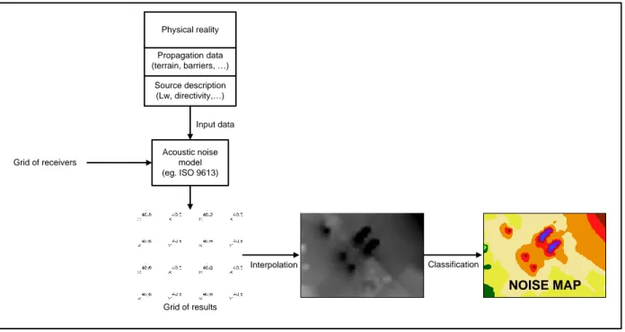
Outdoors noise simulation models have become the most widely used tool for environmental noise assessment. Several models have been developed to estimate noise pollution produced by road traffic, trains, aircrafts and industrial noise sources. All of these models apply the classical methodology that is summarized in Figure 1. A noise model must be configured to make calculation in a grid of spatial locations (receivers). After running the calculation tool, it is obtained a grid of results, which is used for the spatial interpolation(1) of a full map. The final classification of the results is useful for data analysis, comparison to limits, action planning… (2)
Source description (Lw, directivity,…)
Acoustic noise model (eg. ISO 9613) Propagation data (terrain, barriers, …)
Physical reality
Input data
Interpolation Classification
NOISE MAP
Grid of results Grid of receivers
Figure 1. Noise mapping process
An acoustic consultant will have to choose a starting grid of receivers, which is a compromise between accuracy and computational cost. After the model calculation and interpolation process, it is possible to make an estimation of the uncertainty(3,4).
If the uncertainty is small enough, the process is complete at this point. Otherwise, a new finer grid must be chosen. An extra full calculation process must be carried out, obtaining new results with lower uncertainty. This is a very time consuming iterative process(5), which can be improved substantially.
The grid of receivers used for calculations has a great influence in the final results: the thinner the grid (more receivers), the better the results. As the receivers’ density increases, the accuracy of the map is improved, but the computational costs will also increase exponentially.
2
METHODOLOGY
The self-adaptive grids method is based upon the following basis: The isolines are the supporting objects in a noise map, so that if the isolines are perfectly drawn, the map is completely perfect.
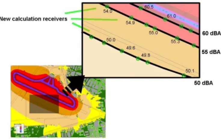
Assuming that this is true, we can derive that the error at any location between two consecutive isolines will be zero. So, the uncertainty in a noise map is produced by the random deviations between the noise level expressed by the isoline and the real value at each location on that line (Figure 2).
Taking this in mind, we can minimize map’s uncertainty setting the focus on finding the correct location of the isolines, instead of getting information about the whole area. We must extend the grid of receivers to perform calculations at those locations where we can extract really useful information, avoiding redundant receivers.
The idea behind this algorithm is to utilize uncertainty sampling for data exploitation(6), which is a concept widely extended in the field of active machine learning(7).
2.1
Noise mapping using self-adaptive grids
To start the practice it is necessary to make a first calculation according to the classical procedure. The starting grid will be a compromise between accuracy and computational cost. After calculation (using the noise model), interpolation and classification (using gis), we get a noise map of a quality that we wished to improve.
To improve the quality of the map, it is necessary to reduce the mean square error (MSE) at the isolines, and we must do it by making new calculations at specific locations on the map.
If we draw the new receivers ―on‖ the isolines (figure 2), we will make them useful in two different ways:
They can be used to make an estimation of the uncertainty of each isoline in the previous iteration.
They will be added to the starting grid for a new spatial interpolation.
Figure 2. New calculation receivers
Thus we get a new map that has been created using all the receivers in the starting grid, and some new receivers, that were placed on the isolines to check if they had been correctly located. So this new map will be more accurate that the previous one.
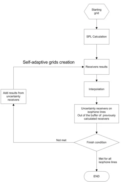
Figure 3. Algorithm for the creation of self-adaptive grids
When using self-adaptive grids, the starting grid can be selected thicker than the required according to the classical procedure (it can be rectangular, triangulated or random). This way, the results in the first iteration can be obtained very quickly.
To check the accuracy of the each isoline, we must locate on it some new receivers. These uncertainty receivers will be calculated using the noise model, and their results will be added to the starting grid to adjust a self-adaptive grid.
Note that the goal of this algorithm is to concentrate the computational effort near the noise isolines. But, it is not strictly necessary to make an uncertainty calculation. Skipping a buffer area near the previous calculated receivers will shorten the calculation process preventing the creation of redundant receivers. However, the estimation of uncertainty may deviate for every iteration, as it is not being calculated for all the necessary sampling. The creation of new receivers and buffers can be easily done using standard GIS methods.
Self-adaptive grids can be very effective in the first iterations. But, while the isolines become more accurate, the new receivers provide less information. So, it must be taken into account in order to define a condition to stop the algorithm. Some of the possibilities for finishing conditions are the following:
The MSE of the isoline is lower than a user defined threshold. For instance, with an independent threshold per each line, the user can focus on those lines that are of interest for action planning.
The improvement on uncertainty of the line is negligible. This will happen when the noise isolines are already well fit. On the other hand, if the initial grid is too coarse, there may be gaps that cannot be detected with self-adaptive grids.
Most of the length of the noise isoline has been previously calculated. If the line is poorly sampled, the estimation of uncertainty (and MSE) could deviate from the real value
The calculated isoline is near the true location, closer than a user’s defined value. This can be estimated by dividing the uncertainty (dB) in the isoline by the map slope (dB/m), converting sound level uncertainty into distance uncertainty.
Other criteria can be used as a function of the expected output results and the target quality of the map.
3
RESULTS
The benefits obtained by using self-adaptive grids depend on each case, as many factors are involved: the number of sources, the source’s strength relation at each receiver, source-receiver distance, the presence of obstacles, the starting grid (which is often a project requirement), or even the size of the simulation.
To illustrate this, we show results for two different examples: a simple point source scenario and a complex multisource industrial site. Acoustic models and calculations have been carried out with Lima 5.02, a software package used primarily for outdoor noise prediction. However, this tool does not allow interpolation of irregular grids, so ESRI ArcInfo Spatial Analyst was used for spatial interpolations.
3.1
Point sound source on an open space
The first example shows results obtained on the simpler scenario: a single point sound source in an open space.
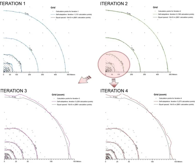
A 100mx100m equally spaced grid was defined and a noise map was obtained. In a first sight, the distant isolines are drawn very accurately, but those situated near the source show a great error. In order to calculate the uncertainty of this map, a new set of simulation receivers is located on every isoline, and the calculation is run for them. Using this new set of results, the MSE of each line is calculated and then, the receivers are merged with those in the starting grid to interpolate a new map (Iteration 1, containing 131 receivers).
The MSE calculated for the starting grid (100mx100m) is lower than 0.1 dB for the lines of 40 and 45dBA. As it is considered not necessary to improve these results, the next iteration only creates new receivers for lines over 50dBA (finish condition).
Figure 4 shows the refinement achieved in this 100x100 regular grid, with each loop. After four iterations, the self-adaptive grid has 275 receivers, and it results in a map with the same accuracy as one that had been calculated using a high resolution regular grid. Figure 4 compares the results obtained by a regular 10mx10m grid (with 2601 receivers), with those obtained using a self-adaptive grid with 131, 198, 239 and 275 receivers (created in iterations 1 to 4).
Figure 5 shows the evolution of the estimated MSE for a few of the noise isolines in relation to the number of iterations and compares these results with those obtained using the thinner 10mx10m grid (2601 receivers).
Figure 4. Isolines obtained applying self-adaptive grids
3.2
Multisource industrial noise
In the case of multisource scenarios or in the presence of obstacles, the starting grid should be at a higher resolution so that gaps can be detected. In these cases, a 5-10% computational effort can reduce uncertainty substantially.
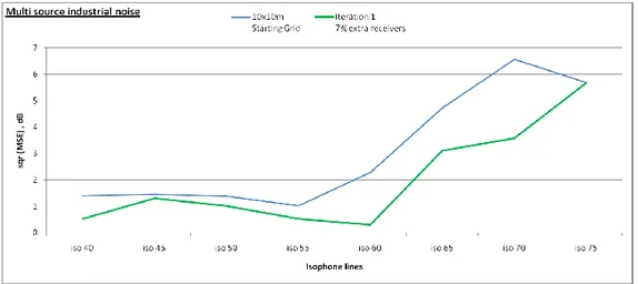
In the following example, a 10mx10m initial grid has been chosen to make a noise map (Figure 6, top right). After one iteration, the addition of 7% receivers (from 5765 to 6173), improves results in most areas of the map (colored area in Figure 6, bottom right). This improvement is only significant in relation to the refinement gained at the location of the isolines (Figure 6, left) and the enhancement produced in their standard uncertainty (Figure 7). Uncertainty of the lines placed closer to the noise source has been enhanced notably (up to 3dB), unlike farther away lines, which see an improvement of less than 0.5 dB.
Figure 6. Efficiency of self-adaptive grid in industrial site noise map
4
CONCLUSIONS
An iterative procedure is implemented to optimize map results by using self-adaptive grids.
The main advantages of using self-adaptive grids include the following:
It is a smart algorithm which analyses previous knowledge to concentrate the calculation effort in those areas where it will be more useful. Because of this, it can provide better results than higher resolution grids, while using fewer receivers for interpolation. Visualization ranges must be chosen from the very beginning because the optimization process focuses on the chosen isolines. If new ranges are selected for visualization, the results will not be optimized, and the uncertainty calculation will be incorrect.
Self-adaptive grids improve the results obtained by any starting grid, no matter the resolution, the number of receivers, or the way they have been located (random, triangulated or equal spaced). The interpolation method used (inverse distance weighting, spline, kriging,..), their parameters or other constrains are also irrelevant, as all of these will improve the accuracy of results as further knowledge (extra receivers) is provided as inputs.
The method based on self-adaptive grids has been proven to be excellent for open spaces with few obstacles. The use of a coarse initial grids, allow the number of calculated receivers to be reduced enormously, while improving the accuracy of the map. The calculation time is drastically reduced, as the number of calculation receivers is reduced. Because of this, this method may be very useful for grid refinement in models that do not consider obstacles in propagation paths (for instance, Integrated Noise Mapping, INM, for airports noise mapping).
Even if a thin initial grid has been chosen, a single iteration of the method will improve map’s accuracy at a low computational cost. As a result, self-adaptive grids have also shown good results when applied to complex acoustic models.
The first iteration also allows proper estimation of the interpolation uncertainty for the starting grid. This allows an independent bias correction for each isoline, instead of additional interpolations.
The weak points of self-adaptive grids can be summarized as follows:
When there are many obstacles, the use of coarse starting grids, may result in the gaps being missed. In these cases, triangular starting grids are preferred.
To reduce calculation times, it has been proposed that the creation of new receivers close to those previously calculated be avoided. Therefore, uncertainty may not be estimated properly for each iteration, as these buffers are excluded from calculations.
When noise maps are calculated for more than one period (for instance, day, evening and night), self-adaptive grids should be used independently for each of these periods. This will improve the effectiveness for each iteration, but will increase the number of extra receivers.
4.1
DISCUSSION
The finishing condition and buffer radio, mentioned in the algorithm, should be further studied in relation to the posterior use of commercial simulation software and according to the final user’s feedback. Depending upon the prediction scenario and map requirements, a selection of parameters that usually works can produce inappropriate results.
The ranges used during the creation of the self-adaptive grids have an influence on the behaviour of the algorithm. Using 5dB ranges requires fewer receivers at each iterative loop. However, using 1dB ranges, will make each loop more effective.
To achieve the best algorithm, it needs to be implemented in sound propagation calculation software and the results studied. The combined effects of the self-adaptive grids, ranges and other acoustic constrains need to be evaluated in order to find a good balance for the initial parameters.
The algorithm for self-adaptive grids has been intended to work in noise maps accompanied by simulation tools. Moreover, self-adaptive grids can also be customized for measurement maps. However, the costs of making new measurements may make this unrealistic.
Other points of discussion and future research include the possibility of using self-adaptive grids for mapping, based on simulations or measurements, in other fields of science.
References
[1] ESRI Inc. Arcgis 9.2 Desktop Help. 2007; Available at: http://webhelp.esri.com/arcgisdesktop/9.2. Accessed 6/17, 2009.
[2] Necessary quality of the input data in the noise mapping methods as a function of expected output results. Noise mapping according to the 2002/49/EC. Target quality and input requirements; 2009.
[3] Methods for quantifying the uncertainty in noise mapping. Managing Uncertainty in Noise Measurement and Prediction; 2005.
[4] Working Group 1 of the Joint Committee for Guides in Metrology. Evaluation of measurement data — Guide to the expression of uncertainty in measurement. 2008.
[5] Optimizing uncertainty and calculation time. Forum Acusticum 2005; 2005.
[6] Lewis D, Catlett J. Heterogeneous uncertainty sampling for supervised learning. 1994:156.