DAMIAN-PAR: a numerical tool for the simulation of wave propagation problems over large scale seismic scenarios based Upon the Finite Element Method

(1)

DAMIAN-PAR: A Numerical Tool for the Simulation of Wave

Propagation Problems Over Large Scale Seismic Scenarios Based

Upon the Finite Element Method

Ricardo Serrano Salazar Escuela de Ingenier´ıa

Universidad EAFIT Medell´ın Colombia

(2)

DAMIAN-PAR: A Numerical Tool for the Simulation of Wave Propagation Problems Over Large Scale Seismic Scenarios Based Upon the Finite Element Method

Ricardo Serrano Salazar

A thesis presented for the degree of Master of Science

Escuela de Ingenier´ıa Universidad EAFIT

(3)

Chapter 1

Introduction

The simulation of earthquakes is necessary to have an understanding about how seismic waves that propagate through earth can a↵ect urban areas sometimes producing catastrophic losses at the surface. Usually, researchers model simplified earthquakes to have a closer understanding of the phenomena; however, realistic simulations of actual earth models and earthquake sources are necessary for an understanding that can be applied to the prevention and management of disasters at a vulnerable region. Realistic simulations of earthquakes provide challenges that are not foreseen in their simplified counterparts, like the modeling of a region that comprises hundreds of kilo-meters and whose materials might have non-linearities or at least be highly heterogeneous. The model can also include a seismic source modeled with high frequencies. The detailed simulation of a model with these complexities implies large computational demands exceeding the standard capabilities of practicing engineers. In other words, to model such problem it’s necessary to develop software that takes advantage of a lot of computational resources in the form of a computer cluster. A computer cluster is a set of computer servers connected through a fast network that can run a single program in all of them at the same time. We call simulations that require and use such computing resources

large scale simulations.

Large scale simulations have been used to reproduce ground motions induced by earthquakes in regions of important seismic activity. For example, Southern California is very vulnerable to earthquakes and researchers usually try to simulate historical earthquakes that occurred in the region using thousands of computing nodes to reproduce the seismograms or to obtain information about the earth’s properties departing from those earthquakes.

Universidad EAFIT, located in Medell´ın which is Colombia’s second largest city, is trying to push projects that make use of APOLO, a new computing cluster with hundreds of computing nodes that is intended for research in several of EAFIT’s key fields. Grupo de Mecanica Aplicada at EAFIT has been working for years solving wave propagation problems and it has seen the acquisition of APOLO as an opportunity to enhance its capabilities and try to appropriate large scale simulation technologies to solve problems with realistic sizes in Aburra’s Valley. The challenges involved from the software development standpoint had kept Grupo de Mecanica Aplicada from doing so.

(4)

in the study of topographic and local site e↵ects in earthquake engineering. The specific tool developed in this work is the 2D version of HERCULES, the 3D end-to-end earthquake simulation tool implemented at Carnegie Mellon University by the Mechanics, Materials and Computing group led by Professor Jacobo Bielak. The 2D code, implemented in this work is part of DAMIAN, the family of numerical simulation programs developed by Grupo de Mecanica Aplicada for the study of wave propagation phenomena in di↵erent contexts. As such, this specific numerical tool has been termed DAMIAN-PAR. This report describes he main contributions of the current work, namely aspects of the specific used finite element algorithm, a validation study, an interpolation scheme proposed for the specific use of large scale seismic scenarios given in terms of velocity models and a large scale simulation of the seismic response of the Aburra Valley using a recently developed crust model for the sedimentary basin underlying the city of Medellin and its main metropolitan area.

1.1 Literature Survey

There are three main numerical methods used for large scale simulations of earthquakes: (i) the finite di↵erence method, (FDM); (ii) the finite element method, (FEM); and (iii) the spectral element method, (SEM). The boundary element method is also an important method for the simulation of the elastic wave equation but it has not been used by many researchers in large scale simulations because it’s difficult to parallelize, it’s limited for highly heterogeneous domains and it’s impractical when considering material non-linearities. The literature survey will examine the three numerical methods often used in large scale simulations of earthquakes and their appropriateness to solve large scale wave propagation problems in earthquake engineering. Each method has had its main contributors who have championed its use and have been determinant to solve the challenges posed by large scale simulations. For each of the methods we will review its strengths and how they compare to other methods.

The Finite Di↵erences Method is the most well known and simple numerical method to approx-imate partial di↵erential equations. Its simplicity allows big computational models to be imple-mented and parallelized without much e↵ort; however, its main drawback is that it needs a regular mesh as input. This is the conclusion of [1], that all approaches that account for heterogeneous models are difficult to implement and have to be adapted to the specific problem. FDM is the most active numerical method for large scale simulations of earthquakes, and has had contributions from several researchers like [2] and [3]. The most important researcher in large scale earthquake simulations using FDM is Prof. Yifeng Cui. In [4] the challenges involved in a large scale simula-tion that required 1.8 billion nodes are described, including modeling, preprocessing, solving and visualizing. In [5], a Magnitude 8 hypothetical earthquake in San Andreas’ fault was simulated with the method, solving a model that required a uniform mesh of about 436 billion 40m3 _cubes.

(5)

(6)

was used originally to simulate problems with 300 million degrees of freedom, which allowed the simulation of regions of 80 x 80 x 80 Km3 _{and frequencies up to 1 Hz. The method has been}

shown to be scalable and has been used in many applications. In [16] it was used to propose an earthquake model from historical earthquake events. Also, in [17] the method solved a problem that required 5 billion elements with frequencies up to 4Hz. The method is the most versatile of all the numerical methods used to solve large scale simulations of earthquakes, having been modified to model the topography of a region in [18], something which can’t be done with FDM or SEM. As a conclusion, the method has shown good results and its versatility makes it very appropriate for the generalization of large scale simulations to di↵erent problems in regions where the materials and the topography are determinant.

1.2 Appropriation of Large Scale Simulations for Wave

Propaga-tion Problems Technology

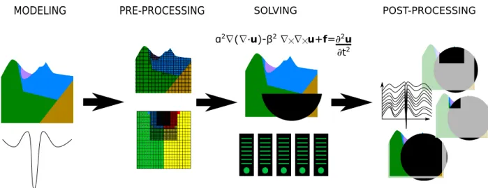
In its basic form, the modelling and simulation of wave propagation problems for earthquake engi-neering consists of the following four steps:

1. First a model of the problem with its geometry, properties and initial conditions is created.

2. The model is converted into a set of computer data structures which hold its discretized information. This is called pre-processing.

3. A solver of the numerical method is run to find an approximate solution to the problem.

4. The solution is presented to the user in a way in which he can do further calculations or take decisions. This is called post-processing.

Each of these four steps provides challenges in large scale simulations that will be addressed in this thesis. A diagram of the tasks that need to be addressed can be found in figure 1.1:

(7)

DAMIAN-PAR is the name of the software created by EAFIT University for the large scale simulation of wave propagation problems in earthquake engineering. DAMIAN-PAR considers the pre-processing, solving and post-processing in a single program because all of the steps need a cluster to be done correctly. The model of Aburra’s Valley, used to test the implementation was created as a separate program, a Community Velocity Model, which not only can be used with DAMIAN-PAR, but can be used with other simulation software. It was used with 3D simulation software in [18]. The following section presents a brief outline of the thesis.

The numerical method chosen in the current thesis was first introduced by Bielak’s group, which in 2D is a quadtree instead of an octree in 2D. The reason is not only the close relationship between EAFIT and CMU, but also that Bielak’s method is the most appropriate to model Aburra’s Valley, which has an aggressive topography and material properties that change very fast. A topography would be very difficult to model with FDM or SEM. Instead, FEM works well with it. The changes in material properties would make FDM and SEM not optimal, FEM can adapt to heterogeneities easily and the quadtree makes it even easier.

The Community Velocity Model, (CVM), was based on an interpretative model of Aburra’s Valley provided by the Geology Department at Universidad EAFIT and compiled in [29] in the form of slices. Then a new interpolation method was developed to have a very smooth transformation between them so the properties would be defined at every point of the geometry. The software developed, called Aburra’s Valley CVM, is also described here.

1.3 Outline of the Master of Science Thesis

The Thesis contains 6 chapters as follows:

1. Introduction: It presents the reasons why the project for the appropriation of large scale

simulations of wave propagation problems in earthquake engineering was carried, a literature survey of numerical methods available to make large scale simulations of earthquakes, and an introduction to the components developed.

2. Theoretical Framework and Strategy of DAMIAN-PAR: It presents the di↵erent

components that constitute DAMIAN-PAR and with the theoretical background behind the tools and the strategies chosen to be able to simulate large scale problems.

3. Validation of DAMIAN-PAR with Classical Problems: Four classical problems are

used to validate DAMIAN-PAR and its approximations. First, low frequency problems are validated against the Boundary Element Method for accuracy. Then, high frequency problems are tested for scalability and performance.

4. Interpolation of 2D Cuts of Earth Formations. Application to the Creation of

Aburr´a’s Valley’s Community Velocity Model: This chapter describes the

implemen-tation of Aburra’s Valley Community Velocity Model. It’s ordered as an article and it’s self contained. It describes the interpolation method which had to be developed in order to inter-polate a set of slices into a full 3D model that describes the elastic properties and topography of Aburra’s Valley.

5. Results of Simulating Slices of Aburra’s Valley: A set of slices of Aburra’s Valley CVM

(8)

(9)

Chapter 2

Theoretical Framework and Strategy

of DAMIAN-PAR

DAMIAN-PAR is the software developed in this thesis to appropriate Large Scale Simulations of Wave Propagation Problems in Earthquake Engineering. DAMIAN-PAR integrates the tasks in Fig. 2.1: (i) pre-processing, (ii) solving and (iii) post-processing. Pre-processing involves reading the configuration of the problem, generating the mesh and applying the boundary conditions and forces to the di↵erent nodes and elements. Solving means finding the values that approximate the solution of the partial di↵erential equation at the nodes of the mesh, at the given times. Post-processing means extracting the solution in formats which can be visualized or analyzed further by a human.

Figure 2.1: Tasks solved by DAMIAN-PAR

(10)

in which the task was executed.

Large Scale Simulations are required when frequencies are too high, feature sizes are too large or material properties are too complex or have low wave velocities. Here the following dimensionless frequency in terms of frequencyf, shear wave propagation velocity and characteristic dimension of the scattererr is defined like:

fo=

f r

. (2.1)

The dimensionless frequency can describe the relative size of a problem with a single parameter. This parameter can be generalized to other problems. In general, the number of elements in the FEM method discretization is proportional to:

✓

f_·F S◆D

(2.2)

where F S is the size of the feature studied (e.g., a valley o canyon) and D is the dimension of the problem, in this case 2. In realistic seismic scenarios, very high dimensionless frequencies are possible when the size of the feature is very large or the materials have a very low wave velocity.

This chapter is divided as follows:

1. Section 2.1 formulates the elastic wave equation with its initial and boundary conditions.

2. Section 2.2 shows the algorithms used to discretize the domain in a quad-tree manner.

3. Section 2.3 shows the finite element discretization of the problem, how it applies to the quad-tree and how loads and boundary conditions are applied.

4. Section 2.4 shows the two forms of post-processing supported by DAMIAN-PAR, generation of synthetic seismograms over determined surfaces (i.e., referred herein as time sheets) and creation of animations; and how they are implemented.

2.1 Problem Statement

Navier’s equations of linear elastodynamics are used to model seismic wave displacements on the earth. Let ui represent the vector field of the three displacement components; let and µ be

Lam´e’s parameters; let⇢be the density distribution; let⇢fi be a time depended body force, which

may represent, for instance a seismic source; let "ij = 1₂(ui,j+uj,i) be the strain tensor and let

⌧ij = "kk ij+ 2µ"ij be the stress tensor. Let⌦be an open bounded domain inR3 with free surface

F S, truncation boundary AB, and outward unit normal to the boundaryni. The initial-boundary

value problem is then written as:

⇢u¨i µui,jj ( +µ)uj,ji=⇢fi in⌦⇥{0tT} (2.3)

=tini =a⇢↵u˙N on AB⇥{0tT} (2.4)

⌧ =_kti nik=b⇢ u˙T on AB⇥{0tT} (2.5)

ti=⌧ijnj = 0 on F S⇥{0tT} (2.6)

(11)

The truncation boundary is defined with the boundary conditions proposed in [19]. In the problem definition is the normal stress,⌧ is the shear stress, ˙uN _{is the normal particle velocity and ˙}_uT _is

the tangential particle velocity while aand bare dimensionless parameters, selected as 1.0 in [19]. P-waves propagate with velocity↵=p( + 2µ)/⇢, and S-waves with velocity =pµ/⇢.

Most realistic seismic problems are approximated by 3D models; however, 2D-based models can be useful to represent certain scenarios by plane strain idealizations and can also be used to interpret an develop conceptual understanding of complex 3D-derived results. This can help us determine the appropriateness of our approximations because the solutions to classical problems are well studied. In plane strain problems all field variables are independent ofx3 and the displacement

in the x3-direction vanishes identically. We set u3 ⌘0 and @/@x3 ⌘0 in (2.3) to obtain the plane

strain equation. Hooke’s law yields the following relations:

⌧↵ = u , ↵ +µ(u↵, +u ,↵) (2.9)

⌧33= u , (2.10)

Where greek indices can assume the values 1 and 2 only. The initial-boundary value problem in 2D is defined as:

⇢u¨↵ µu↵, + ( +µ)u , ↵=⇢f↵ in⌦⇥{0tT} (2.11)

t↵=⌧↵ n = 0 on F S⇥{0tT} (2.12)

=t↵n↵ =a⇢↵u˙N on AB⇥{0tT} (2.13)

⌧ =kt↵ n↵k=b⇢ u˙T on AB⇥{0tT} (2.14)

u↵= 0 on ⌦⇥{t= 0} (2.15)

˙

u↵= 0 on ⌦⇥{t= 0} (2.16)

2.2 Pre-Processing

The preprocessing usually contains the meshing and application of the loads and boundary condi-tions. In Large Scale Simulations, it also contains the partition of the mesh into several processors that will run each one a part of the simulation, sharing the results among them.

A quadtree is a geometric tree data structure that divides the space partitioning each square cell recursively into four equal square cells. As a geometric data structure is a very powerful tool to divide the space and execute geometric queries very fast. As a mesh data structure, the quadtree has been used as a basis for finite element approximation in [20]. Elements are divided into four equal elements until local refinement criteria are satisfied. In Fig. 2.2, the discretization scheme is illustrated.

In the case of seismic wave propagation in heterogeneous media, the criterion for meshing is that there are at least p nodes per local wavelength. As the shear wave velocity is smaller than the pressure wave velocity, the size of the element should behe< 1_{p f}_max. Algorithm 1 creates the

quad-tree using a model of the wave velocity given a point.

(12)

Figure 2.2: Mesh discretized with a Quadtree scheme

Data: Box: the box defined by coordinates: x1,x2,y1,y2, limiting the region to be meshed;

V M(p): The velocity model, returns at the point or air if is above the topography;

f: the maximum frequency of the pulse that will be simulated;

Nper : the number of elements per wave length

Result: M: the quad-tree mesh

begin initialize the mesh

Let max be the highest S-wave velocity of the model;

LetInitial Size _f_N1

per ;

FunctionT arget Size(p) = V M_f(p)_N1

per ;

LetM _{S :S is a square with side Initial Size_^S₂Box_};

end repeat

beginstep that creates the quad-tree mesh

forS |8p2S :V M(p) is air do

M M _{S_};

end

forS |p2S^T arget Size(p) the side of the squareS do

M M _{S_};

M M_[_{the four equal squares dividing S_};

end end

until @S ₂M _|₈p₂S_^T arget Size(p)_ the side of the square S;

(13)

Algorithm 1 would not work for billions of nodes, as the memory required is not available in a single server, but in several of them. The elements have to be partitioned from the beginning and a subset has to be assigned to each processor in the cluster. The quadtree may require several subdivisions of the elements to get to the target element size, creating a node with several elements while others don’t have so many, so the partition is repeated at every meshing step, so a single processor can hold its own subset in memory. Algorithm 2 creates the mesh in parallel.

Data: Box,x1,x2,y1,y2: the box limiting the region to be meshed;

V M(p): returns at the point or air if is above the topography;

f: the maximum frequency of the pulse that will be simulated;

Nper : the number of elements per wave length;

P1, P2, P3, ..., PN: the set of processors,PL will be the local processor ;

Result: M: the distributed quad-tree mesh

begin Parallel initialization

LetBoxL be a rectangular subset ofBoxassigned to PL;

LetML be the mesh initialized as in 1 usingBoxLinstead ofBox;

end repeat

beginParallel quad-tree loop

Create the quad-tree mesh fromML as in 1;

FunctionOD(S ₂M) returns the processor to which the element belongs in an optimal partition;

forPC 2{P1, P2, ...PN}^PC 6=PL do

Send toPC,{S |S2ML^OD(S) =PC};

LetML M {S|OD(S) =PC};

LetML M[{S| the elements received from PC};

end end

until _@S ₂M _|p₂S_^T arget Size(p)_ the side of the square S;

Algorithm 2:Parallelization of the quad-tree mesh creation

(14)

2.3 Finite Element Method Solution to the Problem

The finite element method is used to solve equation 2.3 with bilinear square elements meshed in a quadtree manner. Upon spatial discretization, we obtain a system of ordinary di↵erential equations of the form:

Mu¨+CABu˙ +Ku=f (2.17)

¨

u(0)=u(0)˙ =0 (2.18)

WhereM andK are mass and sti↵ness matrices respectively,f is a body force vector resulting from a discretization of the seismic source model; and damping matrixCAB represents the absorb-ing boundary as in [19]. We use a standard central di↵erence scheme to represent displacement time derivatives yielding an explicit time-marching finite element algorithm. On the other hand, artificially diagonalizing the mass (and damping) matrices to decouple the global system of discrete finite element equations allows us to obtain the following FEM equations:



Mdiag+

t

2 C

AB

diag ut+ t=f



K 2 1

t2M u

t



1

t2M

1 2 tC

AB _ut t

(2.19)

to be solved forut+ t _{using information at}_t_and_t _t_{. In the above algorithm} _t_{is chosen such}

that the P-waves, which are the fastest, traverse an element inn steps. Then t < _n1he

↵.

The discontinuity generated by the hanging nodes is resolved by constraining their field to be the mean of their anchor nodes. This creates a residual that should be added to the anchor nodes. In the case of the explicit finite element method, the following steps have to be added:

1. Sum half of the reactions of the hanging nodes to each neighbor anchor node after the right hand side has been calculated.

2. Set the displacements of each hanging node as the average of its anchor nodes after ut+ t

has been calculated.

The termf was used together with a domain reduction method proposed in [21] to incorporate incoming P and SV plane waves at di↵erent angles. Plane waves have been extensively studied to understand the scattering in terms of basic wave phenomena, and benchmarked solutions are readily available for many plane wave problems. The solutions to plane wave problems hitting di↵erent features, like canyons or valleys, can be used to analyze the appropriateness of our approximations. The DRM is summarized in Fig. 2.3. Most of the following equations have been taken from [21], but some have been modified after our analysis and experiments.

The DRM is a two step method. In the first step, the displacement field u is calculated for a domain ⌦ from an input force f_s that represents a seismic event, and saved in a small frame of elements near DRM. Fig. 2.3a shows DRM which encloses a small region where displacements

(15)

(a) Domain Reduction Method step 1 scheme

(b) Domain Reduction Method step 2 scheme

Figure 2.3: Domain Reduction Method

Fig. 2.3b shows a truncated domain where more complex features have surfaced that would require more complex numerical methods also. The equations that allow the calculation of f_b and f_e are the following:

f_{ef f} =

2 4

f_i

f_b

f_e

3

5=

2 6 4

0

M⌦_be+u¨e0 K⌦

+

be u0e

M⌦_eb+u¨b0+K⌦

+

eb u0b

3 7

5 (2.20)

As M is a diagonal matrix, Mmnu¨n is reduced to 0 if m 6= n leaving previous formula as

simply:

f_{ef f} =

2

4ff_bi

f_e

3

5=

2 6 4

0

K⌦_be+u0_e

K⌦_eb+u0

b

3 7

5 (2.21)

In the case of our work, the displacements ub and ue, were obtained from analytical solutions

for plane SV and P waves incident to a half space, convoluted with Ricker’s Wavelet as formulated in [22]:

Ricker(t) = 1 2⇡2f_peak2 t2 e( ⇡2fpeak2 t2) _(2.22)

(16)

The parallelization of the partial di↵erential equation explicit FEM discretization is very easy because of the way equation 2.19 is organized. First we take the right hand side:

f 

K 2 1

t2M u

t



1

t2M

1 2 tC

AB _ut t _(2.23)

and note that every term is associated with elements, for example M is the sum of the elemental matrices Me. f is also associated with elements in a small frame, from equation 2.21. As such

2.23 can be rewritten like:

f₁



K1 2

1

t2M1 u

t

1 

1

t2M1

1 2 tC

AB

1 ut1 t+

f₂



K2 2 1

t2M2 u

t

2 

1

t2M2

1 2 tC

AB

2 ut2 t+

... (2.24)

Where the subscript represents the element number to which the matrix or vector is associated. This means that the set of elements can be subsetted into several processors that can make the sum independently, and then the full sum can be made afterwards. In the pre-processing step, elements are already assigned and balanced in each processor and the solution of the PDE can be started. The following are the steps considering the quadtree and hanging nodes:

1. Calculate the right hand side at each processor using equation 2.23 and the DRM.

2. Add reactions from other processors at shared nodes.

3. Divide hanging nodes reactions by 2 and add them to its anchor nodes, (local and shared between processors).

4. Calculate ut+ t using equation (2.19).

5. Set the displacements at the hanging nodes as the mean of the displacements at the anchor nodes, (local and shared between processors).

2.4 Post-Processing

The solution, like the mesh and the internal data created by the simulation, is just too big to be handled by the analyst’s personal computer. The solution has to be transformed into something that can be easily handled by the analyst in formats which are of use for him. There are two modes in which the solution can be presented to the analyst in DAMIAN-PAR:

1. Animation mode: It gives the analyst a frame of the solution at a given precision. The frame can be of the whole region modeled or just of a small fraction. For example, the analyst might want to obtain an animation in the metropolitan area of Aburra’s Valley and not in the whole 2D slice modeled. The solution is exported to ParaView where advanced visualizations can be created for further analysis.

(17)

Both modes make use of the quad-tree as a geometrical tree data structure, (opposed to as a mesh data structure), which can make queries very fast. In the first mode, points in a rectangular grid are searched in several processors. We define the quadtree geometrical data structure as follows: LetQT be a data structure with 5 operations:

1. center(QT): returns a pointc which is the center ofQT.

2. upper right(QT): returns the quadtree that contains the elements at the upper right of

center(QT) or empty.

3. upper lef t(QT): returns the quadtree that contains the elements at the upper left ofcenter(QT)

or empty.

4. lower right(QT): returns the quadtree that contains the elements at the lower right of

center(QT) or empty.

5. lower lef t(QT): returns the quadtree that contains the elements at the upper left ofcenter(QT)

or empty.

center(QT) has to be chosen in a way that makes every one of its four quadtree branches disjoint,

an element can’t be divided by a coordinate of the center. A point can be searched in a quadtree at each processor with algorithm 3.

Data: p: Point to be searched;

QT: Quadtree organized in a datastructure;

Result: ep: the element in which pis located

repeat

Letc center(QT);

if QT is a leaf element ethen

if p₂ethen

ep e;

end else

ep ;

end return end

if p(X)> c(X)^p(Y)> c(Y) thenLetQT upper right(QT);

;

if p(X)< c(X)_^p(Y)> c(Y) thenLetQT upper lef t(QT);

;

if p(X)> c(X)^p(Y)< c(Y) thenLetQT lower right(QT);

;

if p(X)< c(X)_^p(Y)< c(Y) thenLetQT lower lef t(QT);

;

until QT =;;

ep ;

(18)

The synthetic seismograms are the progression of the displacements at the surface of the model. As the mesh is arbitrarily partitioned, the points at the surface also have to be searched using the quadtree but with a modification to the algorithm. This time we are interested in finding the highest point of the quadtree. Algorithm 4 finds the highest element which contains the given X coordinate. The algorithm needs a stack which is a data structure with the following operations:

1. pop(ST) returns the object at the top ofST and removes it from the stack.

2. push(ST, A) inserts an object Aat the top of the stack.

3. empty(ST) returns true if the stack is empty.

Data: XC: Coordinate to be searched at the surface;

QT: Quadtree organized in a datastructure;

Result: ex: the highest element that boundsX

begin

Stack definition

end

Let QT be a stack of pointers to quadtrees.;

push(ST, QT);

repeat

LetQT pop(ST);

Letc center(QT);

if QT is a leaf element ethen

if p₂ethen

ep e;

return end end

if XC > c(X)then

push(ST, lower right(QT);

push(ST, upper right(QT);

end

if XC < c(X)then

push(ST, lower lef t(QT);

push(ST, upper lef t(QT);

end

until ¬Empty(ST);

ep ;

Algorithm 4:Algorithm that finds the highest point of a Quadtree given a coordinate

Having found a point in an element, this is transformed to local element coordinates and the value of the displacements at that point is found using the following formula:

u=Huˆ (2.25)

(19)

Chapter 3

Validation of DAMIAN-PAR with

Classical Problems

In this section we conduct low and high frequency validations of the numerical simulator. Valida-tions at low frequencies are targeted at knowing how the correctness of the solution is a↵ected by the di↵erent approximations made to run large scale simulations. Validations at high frequencies are aimed at showing how the program works when stressed with large problems, if it can scale to a large amount of processors and how the time of the solution is a↵ected by using more processors.

3.1 Low Frequency Validations

The validation at low frequencies is done against DAMIAN-BEM-HS, a direct boundary element method software using rigorous half-space Green’s functions developed by Grupo de Mecanica Aplicada at Unversidad EAFIT. BEM is often used in the literature as a benchmark for other methods when analytical solutions are not available because of its sem-analytic character imposed by the Green’s functions and the fact that the radiation boundary condition is exactly satisfied without the need to introduce artificial truncation boundaries.The BEM code has been validated extensively inside Grupo de Mecanica Aplicada.

The four classic validations are shown in Fig. 3.1. The characteristics of the validations are:

1. The rectangular canyon: It’s the most simple validation because it can be approximated perfectly using squared equal elements and because there’s only one material to discretize which means the quad-tree and hanging nodes are not required.

2. The semi-circular canyon: It will show the magnitude of the error involved when discretizing a semi-circular free surface with perfect squares instead of following the path of the curve. It also has a single material to discretize as the rectangular canyon does. It does not use the quad-tree.

3. The rectangular valley: It can be approximated perfectly using squared elements but has two materials with di↵erent wave velocities which makes the quadtree necesary.

(20)

(a) Rectangular Canyon Geometry (b) Semi-Circular Canyon Geometry

(c) Rectangular Valley Geometry (d) Semi-Circular Valley Geometry

Figure 3.1: Geometries for the validations

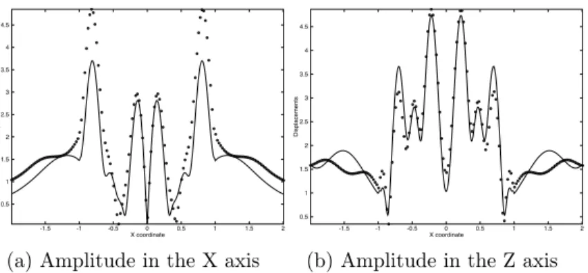
Vertical incidence S-Wave and P-Waves are used against all the models, giving 8 scenarios in total. The incident waves have velocity = 1.0 for the hardest material and = 0.5 for the softest one. Poisson’s ratio is v = 1/3. The peak frequency of Ricker’s pulse is fpeak = 1.0Hz while the

maximum frequency isfmax= 4.0Hz. The amplitude of the incoming SV and P waves is 1.0. The

program is dimensionless and consistency is left to the user.

3.1.1 Rectangular Canyon

The simplest of the geometries to discretize with the quad-tree is the rectangular canyon. In this case there are four sources of di↵raction located in each one of the corners of the canyon that will generate P and SV cylindrical waves and will also generate head waves connecting them. Grazing waves will be generated in the walls of the canyon.

(21)

transfer function for the P-wave. In the following models similar methods will be used to obtain the images, however they will not be explained in detail.

The comparison in time domain shows a perfect correspondence between both DAMIAN-PAR and BEM. The transfer function shows also a very good correspondence with small di↵erences that could be explained by the transformation of the time domain solution to frequency domain, because the frequency is not perfectly 1 but a frequency very close to it. In both cases it’s shown that the rectangular canyon can be perfectly represented by the quadtree discretization, as expected.

(a)t=t1 (b)t=t2 (c)t=t3 (d)t=t4

Figure 3.2: Snapshots of the SV-Wave incident to a rectangular canyon at 0 degrees.

(a) Displacements in the X axis (b) Displacements in the Z axis

Figure 3.3: Synthetic seismograms of the SV-Wave incident to a rectangular canyon at 0 degrees.

Frequency

Surface Location 0

0.5

1

1.5

2

2.5

3

3.5

4 _-1.5 _-1 _-0.5 ₀ _0.5 ₁ _1.5 ₂

(a) Amplitude in the X axis

Frequency

Surface Location 0

0.5

1

1.5

2

2.5

3

3.5

4 _-1.5 _-1 _-0.5 ₀ _0.5 ₁ _1.5 ₂

(b) Amplitude in the Z axis

(22)

(a)t=t1 (b)t=t2 (c)t=t3 (d)t=t4

Figure 3.5: Snapshots of the P-Wave incident to a rectangular canyon at 0 degrees.

Figure 3.6: Synthetic seismograms of the P-Wave incident to a rectangular canyon at 0 degrees.

Frequency

Surface Location 0

0.5

1

1.5

2

2.5

3

3.5

4

-1.5 -1 -0.5 0 0.5 1 1.5 2

Frequency

Surface Location 0

0.5

1

1.5

2

2.5

3

3.5

4

-1.5 -1 -0.5 0 0.5 1 1.5 2

Figure 3.7: Fourier transform of the P-Wave incident to a rectangular canyon at 0 degrees.

-1 0 1 2 3 4

-4 -2 0 2 4 6 8 10

Displacement

Time

-2 -1 0 1 2 3 4

-4 -2 0 2 4 6 8 10

Displacement

Time

(23)

0.5 1 1.5 2 2.5 3

-1.5 -1 -0.5 0 0.5 1 1.5 2

Displacements

X coordinate

0 0.5 1 1.5 2 2.5 3

-1.5 -1 -0.5 0 0.5 1 1.5 2

Displacements

X coordinate

Figure 3.9: Transfer function comparison of the SV-Wave incident to a rectangular canyon.

-0.5 0 0.5 1 1.5 2 2.5 3

-4 -2 0 2 4 6 8 10

Displacement

Time

-2 -1 0 1 2 3 4

-4 -2 0 2 4 6 8 10

Displacement

Time

Figure 3.10: Time domain comparison of the P-Wave incident to a rectangular canyon.

0.2 0.4 0.6 0.8 1 1.2

-1.5 -1 -0.5 0 0.5 1 1.5 2

Displacements

X coordinate

0.5 1 1.5 2 2.5

-1.5 -1 -0.5 0 0.5 1 1.5 2

Displacements

X coordinate

(24)

3.1.2 Semi-Circular Canyon

The geometry of the Semi-Circular Canyon is approximated with squared elements. In this case only two sources of di↵raction located in each corner of the canyon exist. Almost cylindrical P and SV waves are generated by the canyon and they are connected by head waves.

For the SV-wave hitting the semi-circular canyon, Fig. 3.12 shows a few snapshots, fig. 3.13 shows the synthetic seismograms and fig. 3.14 shows the Fourier transform. For the P-Wave, Fig. 3.15 shows a few snapshots, fig. 3.16 shows the synthetic seismograms and fig. 3.17 shows the Fourier transform. Fig. 3.18 shows the comparison for the SV-wave in the time domain while fig. 3.19 shows the comparison in the frequency domain. Fig. 3.20 shows the comparison for the P-wave in the time domain while fig. 3.21 shows the comparison in the frequency domain. The solid line is the simulation with explicit FEM while the circles are the results with BEM.

The comparison in time domain shows a good correspondence between both programs with smaller peaks for BEM. However, in frequency domain we can see that the transfer function of our program is not smooth, even when it’s very close to the BEM function. It presents irregularities that might be explained by the squares approximation to the surface. This was expected for the canyon and it’s the reason why Bielak’s original software only worked for flat simulations. Aburra’s Valley, which is being simulated, has a lot of topography. The solution looks bad at the canyon, but it does not look bad outside of it, and putting aside the lack of smoothness the solution, it’s close enough to that of BEM.

(a)t=t1 (b)t=t2 (c)t=t3 (d)t=t4

Figure 3.12: Snapshots of the SV-Wave incident to a semi-circular canyon at 0 degrees.

(25)

Frequency

Surface Location 0

0.5

1

1.5

2

2.5

3

3.5

4 _-1.5 _-1 _-0.5 ₀ _0.5 ₁ _1.5 ₂

Frequency

Surface Location 0

0.5

1

1.5

2

2.5

3

3.5

4 _-1.5 _-1 _-0.5 ₀ _0.5 ₁ _1.5 ₂

Figure 3.14: Fourier transform of the SV-Wave incident to a semi-circular canyon at 0 degrees.

(a)t=t1 (b)t=t2 (c)t=t3 (d)t=t4

Figure 3.15: Snapshots of the P-Wave incident to a semi-circular canyon at 0 degrees.

Figure 3.16: Synthetic seismograms of the P-Wave incident to a semi-circular canyon at 0 degrees.

Frequency

Surface Location 0

0.5

1

1.5

2

2.5

3

3.5

4 _-1.5 _-1 _-0.5 ₀ _0.5 ₁ _1.5 ₂

Frequency

Surface Location 0

0.5

1

1.5

2

2.5

3

3.5

4 _-1.5 _-1 _-0.5 ₀ _0.5 ₁ _1.5 ₂

(26)

-2 -1 0 1 2 3 4 5

-4 -2 0 2 4 6 8 10

Displacement

Time

-2 -1 0 1 2 3 4

-4 -2 0 2 4 6 8 10

Displacement

Time

Figure 3.18: Time domain comparison of the SV-Wave incident to a semi-circular canyon.

0.5 1 1.5 2 2.5

-1.5 -1 -0.5 0 0.5 1 1.5 2

Displacements

X coordinate

0 0.5 1 1.5 2 2.5

-1.5 -1 -0.5 0 0.5 1 1.5 2

Displacements

X coordinate

Figure 3.19: Transfer function comparison of the SV-Wave incident to a semi-circular canyon.

-0.5 0 0.5 1 1.5 2 2.5 3

-4 -2 0 2 4 6 8 10

Displacement

Time

-3 -2 -1 0 1 2 3 4

-4 -2 0 2 4 6 8 10

Displacement

Time

(27)

0.2 0.4 0.6 0.8 1 1.2

-1.5 -1 -0.5 0 0.5 1 1.5 2

Displacements

X coordinate

1 1.2 1.4 1.6 1.8 2 2.2 2.4 2.6 2.8

-1.5 -1 -0.5 0 0.5 1 1.5 2

Displacements

X coordinate

(28)

3.1.3 Rectangular Valley

The geometry of the rectangular valley is matched perfectly by squares, but the interface between two materials is approximated using the quadtree scheme. In this case waves are reflected and refracted by the inner rectangle, which has a lower wave velocity. Four sources of di↵raction are located in each of the corners of the rectangle and head waves connect the di↵racted P and SV waves inside and outside the region. After the wave inside the lower velocity region is reflected by the free boundary, it hits again the lower border of the valley and gets reflected and refracted again. Waves generated by the sources of di↵raction also remain in the valley being reflected and refracted so the wave requires a long time to be disappear completely.

For the SV-wave hitting the rectangular valley, Fig. 3.22 shows a few snapshots, fig. 3.23 shows the synthetic seismograms and fig. 3.24 shows the Fourier transform. For the P-Wave, Fig. 3.25 shows a few snapshots, fig. 3.26 shows the synthetic seismograms and fig. 3.27 shows the Fourier transform. Fig. 3.28 shows the comparison for the SV-wave in the time domain while fig. 3.29 shows the comparison in the frequency domain. Fig. 3.30 shows the comparison for the P-wave in the time domain while fig. 3.31 shows the comparison in the frequency domain. The solid line is the simulation with explicit FEM while the circles are the results with BEM.

In time domain, the correspondence is good between our solution and BEM at the beginning, but starts to become less good with every reflection. This is magnified in the transfer functions, that show that the correspondence is not very good between BEM and DAMIAN-PAR. The discrepancies were not expected as the approximation to the geometry was supposed to be perfect and prove the correctness of the quadtree.

(a)t=t1 (b)t=t2 (c)t=t3 (d)t=t4

Figure 3.22: Snapshots of the SV-Wave incident to a rectangular valley at 0 degrees.

(29)

Frequency

Surface Location 0

0.5

1

1.5

2

2.5

3

3.5

4 _-1.5 _-1 _-0.5 ₀ _0.5 ₁ _1.5 ₂

Frequency

Surface Location 0

0.5

1

1.5

2

2.5

3

3.5

4 _-1.5 _-1 _-0.5 ₀ _0.5 ₁ _1.5 ₂

Figure 3.24: Fourier transform of the SV-Wave incident to a rectangular valley at 0 degrees.

(a)t=t1 (b)t=t2 (c)t=t3 (d)t=t4

Figure 3.25: Snapshots of the P-Wave incident to a rectangular valley at 0 degrees.

Figure 3.26: Synthetic seismograms of the P-Wave incident to a rectangular valley at 0 degrees.

Frequency

Surface Location 0

0.5

1

1.5

2

2.5

3

3.5

4 _-1.5 _-1 _-0.5 ₀ _0.5 ₁ _1.5 ₂

Frequency

Surface Location 0

0.5

1

1.5

2

2.5

3

3.5

4 _-1.5 _-1 _-0.5 ₀ _0.5 ₁ _1.5 ₂

(30)

-2 -1 0 1 2 3 4

-4 -2 0 2 4 6 8 10

Displacement

Time

-0.5 0 0.5 1 1.5 2 2.5

-4 -2 0 2 4 6 8 10

Displacement

Time

Figure 3.28: Time domain comparison of the SV-Wave incident to a rectangular valley.

0.5 1 1.5 2 2.5 3 3.5 4

-1.5 -1 -0.5 0 0.5 1 1.5 2

Displacements

X coordinate

0.5 1 1.5 2 2.5 3 3.5

-1.5 -1 -0.5 0 0.5 1 1.5 2

Displacements

X coordinate

Figure 3.29: Transfer function comparison of the SV-Wave incident to a rectangular valley.

-0.5 0 0.5 1 1.5 2 2.5

-4 -2 0 2 4 6 8 10

Displacement

Time

-3 -2 -1 0 1 2 3

-4 -2 0 2 4 6 8 10

Displacement

Time

(31)

0.5 1 1.5 2 2.5 3 3.5 4 4.5

-1.5 -1 -0.5 0 0.5 1 1.5 2

Displacements

X coordinate

0.5 1 1.5 2 2.5 3 3.5 4 4.5

-1.5 -1 -0.5 0 0.5 1 1.5 2

Displacements

X coordinate

(32)

3.1.4 Semi-Circular Valley

The geometry of the semi-circular valley is approximated with squares and the interface between both materials is approximated with the quadtree scheme. In this case waves are reflected and refracted by the inner semi-circle, which has a lower wave velocity. Refracted waves inside the lower velocity region create a concave wave. This model only has two sources of di↵raction are located at each of the corners of the canyon. Like the rectangular canyon, the waves hit the boundary several times reflecting and refracting until they are weak enough.

For the SV-wave hitting the rectangular valley, Fig. 3.32 shows a few snapshots, fig. 3.33 shows the synthetic seismograms and fig. 3.34 shows the Fourier transform. For the P-Wave, Fig. 3.35 shows a few snapshots , fig. 3.36 shows the synthetic seismograms and fig. 3.37 shows the Fourier transform. Fig. 3.38 shows the comparison for the SV-wave in the time domain while fig. 3.39 shows the comparison in the frequency domain. Fig. 3.40 shows the comparison for the P-wave in the time domain while fig. 3.41 shows the comparison in the frequency domain. The solid line is the simulation with explicit FEM while the circles are the results with BEM.

The correspondence is good between our solution and BEM at the beginning, but starts to become less good with every reflection. However, the solution does not seem to be worst than the solution of the rectangular valley, it’s actually better as shown by the frequency domain comparison. This was unexpected because the semi-circular valley has the quadtree approximation and also models the interface as perfect squares. The approximation with squares is actually good enough to represent not squared geometries in this case, and not only because the interfaces are not well known as explained by Bielak.

(a)t=t1 (b)t=t2 (c)t=t3 (d)t=t4

Figure 3.32: Snapshots of the SV-Wave incident to a semi-circular valley at 0 degrees.

(33)

Frequency

Surface Location 0

0.5

1

1.5

2

2.5

3

3.5

4 _-1.5 _-1 _-0.5 ₀ _0.5 ₁ _1.5 ₂

Frequency

Surface Location 0

0.5

1

1.5

2

2.5

3

3.5

4 _-1.5 _-1 _-0.5 ₀ _0.5 ₁ _1.5 ₂

Figure 3.34: Fourier transform of the SV-Wave incident to a semi-circular valley at 0 degrees.

(a)t=t1 (b)t=t2 (c)t=t3 (d)t=t4

Figure 3.35: Snapshots of the P-Wave incident to a semi-circular valley at 0 degrees.

Figure 3.36: Synthetic seismograms of the P-Wave incident to a semi-circular valley at 0 degrees

Frequency

Surface Location 0

0.5

1

1.5

2

2.5

3

3.5

4 _-1.5 _-1 _-0.5 ₀ _0.5 ₁ _1.5 ₂

Frequency

Surface Location 0

0.5

1

1.5

2

2.5

3

3.5

4 _-1.5 _-1 _-0.5 ₀ _0.5 ₁ _1.5 ₂

(34)

-4 -2 0 2 4 6

-4 -2 0 2 4 6 8 10

Displacement

Time

-0.5 0 0.5 1 1.5 2 2.5

-4 -2 0 2 4 6 8 10

Displacement

Time

Figure 3.38: Time domain comparison of the SV-Wave incident to a semi-circular valley.

0.5 1 1.5 2 2.5 3 3.5 4 4.5

-1.5 -1 -0.5 0 0.5 1 1.5 2

Displacements

X coordinate

0.5 1 1.5 2 2.5 3

-1.5 -1 -0.5 0 0.5 1 1.5 2

Displacements

X coordinate

Figure 3.39: Transfer function comparison of the SV-Wave incident to a semi-circular valley.

-0.5 0 0.5 1 1.5 2 2.5

-4 -2 0 2 4 6 8 10

Displacement

Time

-4 -3 -2 -1 0 1 2 3 4

-4 -2 0 2 4 6 8 10

Displacement

Time

(35)

1 2 3 4 5

-1.5 -1 -0.5 0 0.5 1 1.5 2

Displacements

X coordinate

1 1.5 2 2.5 3 3.5 4 4.5 5

-1.5 -1 -0.5 0 0.5 1 1.5 2

Displacements

X coordinate

(36)

3.2 High Frequency Validations

At high frequencies what is important is the scalability of the solution. High frequencies are not realistic for most seismic events, as the range of frequencies usually goes up to 5 Hz. However, we are interested with the size of the problem as defined in section 2 which is related to the non-dimensional frequency. As such the dimensionless frequency for the semi-circular canyon is defined as:

f0=

f r

2 (3.1)

So given a problem it’s possible that changed to a non-dimensional frequency it might seem unreal-istic, but it’s not when wave velocity is low or the feature’s size is large. We made 8 simulations, this time with peak frequencyfpeak = 16 and maximum frequencyfmax= 64. We used 320 Quad-Core

AMD OpteronRProcessor 2380 to simulate the problem and set 4 hours of maximum time. We

present the result only in snapshots, number of degrees of freedom, (DOFs), and time, as it’s very difficult to analyze synthetic seismograms or other information at such high frequencies and BEM is not capable of simulating such high frequencies to compare.

(37)

(a)t=t1 (b)t=t2

(c)t=t3 (d)t=t4

(e)t=t5 (f) t=t6

(g)t=t7 (h)t=t8

(38)

(a)t=t1 (b)t=t2

(c)t=t3 (d)t=t4

(e)t=t5 (f) t=t6

(g)t=t7 (h)t=t8

(39)

(a)t=t1 (b)t=t2

(c)t=t3 (d)t=t4

(e)t=t5 (f) t=t6

(g)t=t7 (h)t=t8

(40)

(a)t=t1 (b)t=t2

(c)t=t3 (d)t=t4

(e)t=t5 (f) t=t6

(g)t=t7 (h)t=t8

(41)

(a)t=t1 (b)t=t2

(c)t=t3 (d)t=t4

(e)t=t5 (f) t=t6

(g)t=t7 (h)t=t8

(42)

(a)t=t1 (b)t=t2

(c)t=t3 (d)t=t4

(e)t=t5 (f) t=t6

(g)t=t7 (h)t=t8

(43)

(a)t=t1 (b)t=t2

(c)t=t3 (d)t=t4

(e)t=t5 (f) t=t6

(g)t=t7 (h)t=t8

(44)

(a)t=t1 (b)t=t2

(c)t=t3 (d)t=t4

(e)t=t5 (f) t=t6

(g)t=t7 (h)t=t8

(45)

Table 3.1 shows the number of DOFs and time for each one of the models. As the wave velocity and geometry are defined the same for incident SV-Waves and P-Waves, the number of DOFs is the same for both waves. Time depends on the number of DOFs and the time simulated, which was 12 seconds. The number of steps for all the models was automatically calculated as 64.000. The tests show that the algorithm can be scaled to use hundreds of computing nodes. Problems of larger sizes would require even more computing nodes but could be in theory scaled. 3 dimensional problems require more DOFs but not more steps as they depend on the side of the elements, (squares or cubes), which does not grow with the dimension, so scaling the problem to 3D would require more computing nodes but not more time.

Table 3.1: Number of DOFs and time for each model.

Model DOFs Time

Rectangular Canyon SV-Wave 51.583.112 6.492s P-Wave 51.583.112 6.564s

Semi-Circular Canyon SV-Wave 51.965.042 7.275s P-Wave 51.965.042 6.698s

Rectangular Valley SV-Wave 58.696.002 7.496s P-Wave 58.696.002 7.644s

Semi-Circular Valley SV-Wave 57.550.134 7.510s P-Wave 57.550.134 7.680s

The semi-circular canyon atfpeak = 8 Hz,fmax= 32 Hz, was evaluated to know the scalability

of the program. Fig. 3.50 shows the times of the solutions when the number of processors is increased from 40 to 240 processors. The curve was fitted to the functionT ime=k⇤ 1

P rocessors n

(46)

500 1000 1500 2000 2500 3000 3500 4000

0 50 100 150 200 250

Time(s)

Number of Processors

(47)

Chapter 4

Interpolation of 2D-cross Sections

from Earth Crust Formations:

Application to the Construction of

the Community Velocity Model for

the Aburr´

a Valley

4.1 Abstract

A Community Velocity Model (CVM), is a computer program and its data files that provide in-formation about earth’s elastic properties from the surface to a given depth. CVMs are necessary to accurately predict the outcome of an earthquake using large scale simulations. Aburra’s Val-ley interpretative geological model was created as an starting point of information about earth’s formations and is comprised of several 2D slices, each one with di↵erent formations delimited by polygons. Interpolating these slices is necessary but there are 3 characteristics that make those slices difficult to interpolate: (i) there are many formations, (ii) slices are far and have a far geom-etry and (iii) the topology of the slices is very di↵erent. We propose an algorithm that is adequate to solve the interpolation problem with the previous constraints and shows good visual results of progression between slices. The model is adequate to create the CVM and was used to simulate earthquakes in Aburra’s Valley taking into account the topography of the region.

4.2 Introduction

(48)

is Southern California Earthquake Center’s, (SCEC’s CVM), which describes the elastic properties of Southern California, [25]. It has information up to 100 Km in depth from inverse tomographic models into one single 3D model, [26, 27, 28]. The CVM is arranged in voxels, cubic boxes that contain the value of a formation, [25]. These voxels are arranged with di↵erent precisions with information built from inversion methods and tomographic iterations.

The present work creates a starting version of a Community Velocity Model for Aburra’s Valley using the information present in [29]. This model will be used to simulate earthquakes and the e↵ect of topography in exiting numerical methods. The interpretative model created in [29] consists of several images of the earth perpendicular to the surface called slices. This representation is the most used form by geologists that construct interpretative models and is also is used in 2D geological surveys. Interpolation is then required to have a full 3D model where a property of the material is defined everywhere. However, current interpolation methods are not useful for the problem at hand which has three characteristics: (i) there are many formations, (ii) slices are far and have a far geometry and (iii) the topology of the slices is very di↵erent. A complete, (to the author’s understanding), literature survey that shows the necessity of a new interpolation method that accounts for these 3 constraints, can be found in section 4.3.

We propose a new method to interpolate slices of earth formations, coming from interpretative models or other models where inter-slice distances are sufficiently large, to create a full 3D model of a region. The paper is divided as follows: (i) we review the methods that have been proposed in several fields to interpolate slices and why they were not appropriate to solve the problem at hand in 4.3, (ii) we explain the rationale behind our approach and propose a two-step algorithm to solve the problem in section 4.4, (iii) we review the results achieved when using the algorithm to interpolate the information in the interpretative model of Aburra’s Valley in section 4.5 and (iv) we show our conclusions about the algorithm and its results in section 4.6.

4.3 Review of Methods to Interpolate Slices into a Full 3D Model

A slice is the image composed by the set of points with a scalar value, each point belongs to a formation. In a slice, many di↵erent formations exist. Two di↵erent polygons can enclose the same formation in the same slice also. The points are in a plane perpendicular to the surface of the earth, and the given formation is a measure or an expertly guessed value which are difficult to obtain. The slice is delimited by the topography which can be easily obtained with precision. The problem we are studying is obtaining values of formation for points that are between the slices, given slices that are sampled far apart but whose formations are presumed to have continuity. Inter-slice distance for Aburra’s Valley interpretative model is 2 Km.

Commercial software sometimes brings features to interpolate slices into a 3D triangulation that can be used for querying points inside regions. Fig. 4.1 is the result of the interpolation made using software RhinoR_{. This result shows intersections of the triangulations that are incorrect for} a CVM. Fig. 4.2 shows a cut made to Rhino’s interpolation. It shows that there are empty regions or formations that are also incorrect in the creation of the CVM.

(49)

(a) Perspective View of the solid interpolated.

(b) Top view of the solid in-terpolated.

Figure 4.1: Perspective and top views of the solid Modeled with RhinoR _{which shows intersections}

Figure 4.2: Cut of the solid that shows holes

2 nearest oposite vertices of the voxel and trilinear interpolation, [30], which uses information from the 8 vertices of the voxel. Higher order interpolations use near voxels to compute the interpolation of the value with a higher order function, for example tricubic, [33], quadratic, [34], and bicubic, [35]. These methods rely on small transitions from one slice to another. If the same formation does not occur between the two sides of the used voxels, the transition between the two formations is not kept. Another shortcoming of voxel algorithms is that they also rely on the pixel distance to inter slice distance ratio. This assumption is broken when slices are vector images, in which the formations can be sampled with any granularity.

For geophysics and earth resources’ exploration there is an entire field that focuses on statisti-cally analyzing and interpolating spatial datasets called geostatistics. In this field, the techniques to interpolate are called Kriging. For a detailed introduction to geostatistics see [36]. Kriging is used for interpolation of slices in [37]. Because it’s a statistical tool, it has optimality guarantees. In practice, [37] shows that Kriging slices relies on the information of the voxel or the neighborhood of voxels, as the previous voxel based methods so it’s limited when inter slice distance is big.

Shape-based interpolation algorithms are another class of methods, [38, 39]. These algorithms start with a binary image, where the object is one and the outside is 0. Then they convert the image to a grey-scale image based on the distance to the boundary of the object, positive inside and negative outside. An image interpolation method is then used to find the boundaries inter-slices. The problem with this algorithm is its binary nature, only object and outside of object are recognized. It’s not possible to have more than one formation.

(50)

to look at the tissues from a di↵erent perspective or to have a 3D planning of a surgery. The most used techniques to obtain isosurfaces, (which are the collection of points of a same value within a volume of space), and from those interpolate the value in the region between the slices, is the marching cubes algorithm in [40]. The algorithm is designed for visualization, so incorrect topology is acceptable as long as it’s correct enough to visualize. The marching cubes and other reconstruction algorithms have been extended to create topologically correct surfaces, for example in [33] and [41]. Both algorithms deal with the problem of creating a surface which is locally topologically equivalent to a disk in every point, they don’t deal with the problem of creating shapes from samples that are topologically equivalent to the original. A complete survey of the marching cubes algorithm was published in [42]. These algorithms also use voxels, but to create isosurfaces. They can only be locally correct and don’t give guarantees about the shape so they are not appropriate for big changes in the geometry or topology.

Other kind of techniques to create isosurfaces use pattern recognition techniques and triangu-lations like Delaunay’s, [43, 44, 45]. Unlike previous algorithms which relied on the voxels and discretization, these algorithms can interpolate between very di↵erent and separated slices. They also can ensure the topology is respected in cases like branching and merging. Like the shape based interpolation methods, these algorithms rely on a single formation, in this case bone. If more than one formation is interpolated, the triangulations would overlap and form intersections and holes, like in Figs. 4.1 and 4.2.

4.4 Interpolation Technique for Aburr´

a’s Valley CVM

The concept of interpolating a value from a set of measures is closely related to the general problem of shape reconstruction. Generally, topology and geometry are used as indicators for correctness of an algorithm since [46, 47]. A complete treatment of computational topology and its application to shape and surface reconstruction was published in [48]. A shape is said to be well reconstructed from sample points if it’s homeomorphic to the original sampled shape and geometrically is as close as possible. Let SA and SB be two geometric shapes, SA is homeomorphic to SB if there is a

functionf :SA!SB such thatf is bijective andf and its inverse are continuous. Intuitively, two

shapes are homeomorphic if one can be created from another by stretching and bending but not by cutting or glueing. Fig. 4.3 shows two homeomorphic shapes.

(a) Shape SA which is a

slice with 3 formations.

(b) Shape SB which is

(51)

If two shapes are homeomorphic it means that they might be slightly deformed until they are converted into one another. If two slices are homeomorphic it means that isosurfaces can be con-structed between them that connect every loop to another loop in the adjacent surface. Otherwise, by definition, connecting two shapes is mathematically impossible without a topological transition, because at some point the geometry would have to be glued or cut. That’s why commercial soft-ware reconstruction of slices fails in such cases, as in Fig. 4.2. However, we can see that even when topology can change, the transition can be simple, as in Fig. 4.4.

(a) ShapeSC which is not

homeomorphic toSBbut is

a transformation of it.

(b) ShapeSD which is not

homeomorphic toSBbut is

a transformation of it.

Figure 4.4: The shapes are not homeomorphic to those of Fig. 4.3, but they can be transformations from them.

Unlike triangulations that can overlap, leave holes or even have local topological inconsisten-cies, real distance functions are well defined at every point of the space. That’s the reason why they are to chose with problems that, unlike visualization, require a perfect topology. Delaunay’s triangulation is possibly the most important geometrical data structure. It’s dual is Voronoi’s di-agram which is the set regions that is closer to each point, (called site), than to any other point. In computational geometry, Delaunay’s triangulation is the best definition of closeness available. Proof of this is that Delaunay’s triangulation contains the euclidean minimum spanning tree, the relative neighborhood graph, and the nearest neighbor graph. For a complete description see [49]. Delaunay’s triangulation, with the appropriate topological transition, is used in many isosurface interpolation papers as main resource. Unlike those papers, we use Delaunay Triangulation to find which polygons of two di↵erent slices match. After that matching, we use a real distance function that follows the direction of the polygons. The real distance function is defined at every point between the slices and can be compared to the same distance function to other matching polygons. Given a triangulation, T, two polygons match according to their connected length. A polygon is denoted asP =_{L1, L2, . . . , LN}: a set of loops, interior and exterior that encloses a formation,

denoted asF ormation(P). The formation consists of a certain number of rock strata that have com-parable lithology, facies or other similar properties. The loop is a closed line L={p1, p2, . . . , pN}

where (p1, p2),(p2, p3), . . . ,(pN, p1) are segments. The connected length of two polygons with the

same formation, denoted asConLen(P1, P2), is the sum of the length of the segments a loop that

belongs to P1 which are part of a triangle of the triangulation that has its opposite vertex in P2.

(52)

Data: Two slices, IA,IB

Result: M atched, a set of pairs of polygons in opposite slices that match

Obtain the Delaunay Triangulation T of both slices;

for P1, P2 :ConLen(P1, P2)6=; do

if ₈PJ 2IA, ConLen(PJ, P2)< ConLen(P1, P2)^

8PK 2IB, ConLen(P1, PK)< ConLen(P1, P2) then

M axLen(P1, P2) ConLen(P1, P2)

end end

Let M atched _{(P1, P2) :M axLen(P1, P2)6=;};

Let N otM atched _{P1:8P2, M axLen(P1, P2) =;};

for Every polygon P1 in N otM atcheddo

if ₉P2 |ConLen(P1, P2)>0 then

LetP2 the polygon with maximum connected length toP1;

LetM atched M atch[{(P1, P2)};

N otM atched N otM atched _{P1};

end end

for P1 2N otM atcheddo

LetP2 be the matched neighbor that shares more arc length withP1;

AddP1 toP2;

end

Algorithm 5:Find a match for every polygon

The loop pairing can be a costly operation so it’s not done at the same time that the CVM is run. Preprocessing is done between every consecutive pair of slices and saved independently. That is, if sliceIB has some loops merged when matching with sliceIA, those same loops are not merged

when matchingIBandIC, the loops start from scratch. The information saved by the preprocessing

algorithm is the set of loops and matches in IA and IB after the algorithm has finished.

The polygon matching is created to find a direction in which two polygons that are distant are related. After matching the polygons, a vector~v is found as~v =c1 c2, the di↵erence between

the centroids of polygons P1 and P2. For any point p we find the intersection between p+~v and

(53)

Data: A point pwith three spacial coordinates, px,py,pz

Result: The formationF ormation(p) in which that coordinate lies

if p is below the topography then

LetF ormation(p) air.

end

Let IA,IB be the pair of consecutive slices such that the point lies between them;

for (P1, P2)2M atcheddo

Let~v be the vector between the centroids ofP1 and P2. LetqA be the intersection

between the plane that containsIA and p+~v;

LetqB be the intersection between the plane that containsIB and p+~v;

if qA inside P1 then

Letd1 0;

else

Letd1 be the distance toP1; end

if qB inside P2 then

Letd2 0; else

Letd2 be the distance toP2; end

LetDistance(P1, P2) ⇣1 kqA pk

kqA qBk

⌘

d1+⇣1 kqB pk

kqA qBk

⌘

d2;

end

Let F ormation(p) minDistance(P1, P2);

Algorithm 6:Find a formation given a point inside the interpolated region

Wave velocities are the result of combining the formation in with geophysical considerations which are outside of the scope of this paper.

4.5 Results

(54)

(a) Interpolation at coordinate Y = 1189500

(b) Interpolation at coordinate Y = 1189700

(c) Interpolation at coordinate Y = 1189900

(d) Interpolation at coordinate Y = 1190100

(e) Interpolation at coordinate Y = 1190300

(f) Interpolation at coordinate X = 1190500

(g) Interpolation at coordinate Y = 1190700

(h) Interpolation at coordinate Y = 1190900

(i) Interpolation at coordinate Y = 1191100

(j) Interpolation at coordinate Y = 1191300

(k) Interpolation at coordinate Y = 1191500

(55)

4.6 Conclusions and Future Work

We presented and solved the problem of interpolating the information of an interpretative model for Aburra’s Valley into a Community Velocity Model. The resultant algorithm is very simple and fast for formation querying. It can be parallelized, however as it’s used as a an input to a mesher, it needs to be run by several processes independently and it’s better to keep it single threaded. This CVM is very useful to create more complicated ones from tomographic models, as SCEC’s, which makes it a very important starting point for having an accurate and complete description of the earth below the surface in Aburra’s Valley. The algorithm is very general, so it can be used with models of other regions to create simple CVMs which allows them to comprehend seismic events easily.

As a main conclusion it was shown that it’s possible to formulate an algorithm to interpolate slices into a full 3D model that can be used with an automatic mesher, instead of a human interpreter as in the case of algorithms for visualization. The algorithm can interpolate changing topology, distant geometry and several formations. Previous algorithms could only solve two of the three problems at the same time.