Variable structure control with chattering elimination and guaranteed stability for a generalized T-S model

Variable Structure Control with chattering elimination and

guaranteed stability for a generalized T-S model

Basil Mohammed Al-Hadithi , Antonio Javier Barragan , Jose Manuel Andujar , Agustin

Jimenez

A B S T R A C T

In this paper, a fuzzy based Variable Structure Control (VSC) with guaranteed stability is presented. The main objective is to obtain an improved performance of highly non-linear unstable systems. The main contribution of this work is that, firstly, new functions for chattering reduction and error convergence without sacrificing invariant properties are proposed, which is considered the main drawback of the VSC control. Secondly, the global stability of the controlled system is guaranteed.

The well known weighting parameters approach, is used in this paper to optimize local and global approximation and modeling capability of T-S fuzzy model.

A one link robot is chosen as a nonlinear unstable system to evaluate the robustness, effectiveness and remarkable performance of optimization approach and the high accuracy obtained in approximating nonlinear systems in comparison with the original T-S model. Simulation results indicate the potential and generality of the algorithm. The application of the proposed FLC-VSC shows that both alleviation of chattering and robust performance are achieved with the proposed FLC-VSC controller. The effectiveness of the proposed controller is proven infront of disturbances and noise effects.

1. Introduction

VSC is naturally attractive to control engineers because its basic concepts are rather easy to understand and has given satisfac-tory performance in many practical areas of industrial applications. It has attracted interest recently because a fast calculation and switching action have been realized through the progress of micro and power electronics. The main mode of VSC operation is sliding mode (SM) control.

The basic VSC feature is to drive the state trajectory towards a sliding plan previously determined by computing the feedback con-trol structure. It is desirable to simultaneously: (a) reach the sliding plane fastly; (b) maintain the trajectory close to it; and (c) reduce the number of switchings between structures (chattering). How-ever, reaching the sliding plane fast implies also a fast departure, unless a frequent switching between structures is allowed.

Motivated by observation on similarity between Fuzzy Logic Control (FLC) rules and VSC, the robustness of the VSC has been analyzed for nonlinear dynamic systems in this paper. As results, the asymptotic behavior of the VSC system can be clarified and the relationship between the design parameters and the tracking performances of the control system is addressed explicitly. The relationship is important since it gives guidance on the design parameters of the control system to achieve the specified control performances [7,9-11,37].

SM are used to determine best values for parameters in FLC rules. As robustness is inherent in VSC with SM, robustness in FLC can be improved. The motivation behind this scheme is to combine the best features of FLC and VSC to achieve rapid and accurate tracking control of a class of nonlinear systems [4,8,20,21,23,27,35].

In this paper, a design of FLC-VSC is presented based on T-S fuzzy model [32]. We will show how VSC can be improved for actual implementation by introduction of fuzzy rules. We will also develop a methodology for designing a fuzzy rule based controller to smooth the control input for a general class of VSC's.

Nonlinear control systems based on the T-S fuzzy model [32] have attracted quite attention during the last twenty years (e.g., see [2,3,5,6,16,22,38]). It provides a powerful solution for develop-ment of function approximation, systematic techniques to stability analysis and controller design of FLC systems in view of fruitful conventional control theory.

This fuzzy modeling method presents an alternative technique to represent complex nonlinear systems [42] and reduces the num-ber of rules in modeling higher order nonlinear systems [32,6].

T-S fuzzy models are proved to be universal function approx-imators as they are able to approximate any smooth nonlinear functions to any degree of accuracy in any convex compact region [15,22,33,42]. This result provides a theoretical foundation for applying T-S fuzzy models to represent complex nonlinear systems approximately. But it was clearly shown that the number of fuzzy rules increases as the approximation error tends to zero [19]. This exponential growing cannot be eliminated, so it becomes difficult to make use of the universal approximation property of T-S fuzzy modeling for practical purposes. Moreover, if the number of rules is bounded, the resulting set of functions is nowhere dense in the space of approximated functions [36]. These conflicting objectives have motivated researchers to find a balance between the specified accuracy and the computational complexity of the resulting fuzzy model.

In [26], the authors proposed to obtain the best features of Mamdani and T-S models by using an affine global model with function approximation capabilities, which combines approach capacity and local interpretability. Universal approximation prop-erties of Mamdani fuzzy model are well known. On the other hand, Takagi-Sugeno fuzzy model with affine consequent was thought to be a local approximator of the dynamics. However, it can also be tuned to be an universal approximator, but losing its local interpretation. In [26], an innovative affine global model with universal approximation capabilities which maintains local interpretation is introduced. The suggested model is composed of variant coefficients which are independently governed by a zeroth order fuzzy inference system. This novel model can be considered a generalization of Takagi-Sugeno affine fuzzy model, and is based on decoupling the dynamic parameters of the system at the fuzzi-fication step. The authors have demonstrated how this new model can exactly match non-linear functions expressed either as product form or additive form.

In [14] new and efficient two approaches are presented to improve the local and global estimation of T-S fuzzy model. The main problem is that T-S identification method cannot be applied when the MFs are overlapped by pairs. The approaches developed can be considered as a generalized version of T-S method with optimized performance.

Several methods are used to deal with the problem of optimizing MFs, which are either derivative-based or derivative-free meth-ods. The derivative free approaches are desirable because they are more robust than derivative-based methods with respect to find-ing global minimum and with respect to a wide range of objective functions and MFs types. The drawback is that they converge more slowly than derivative-based techniques [34]. On the other hand, derivative-based methods tend to converge to local minima. In addition, they are limited to specific objective functions and types of inference and MFs. The most common approaches are: gradient descent [28], least squares [30], back propagation [40] and Kalman filtering [29].

The estimation methods presented in this paper are character-ized by the high accuracy obtained in approximating nonlinear systems locally and globally in comparison with the original T-S model. A fuzzy FLC-VSC is proposed in order to show the effec-tiveness of the estimation method developed here in control applications.

The rest of the paper is organized as follows. An introduction to FLC-VSC is presented in Section 2. A new method for chattering elimination is developed in Section 3 (which is considered the main drawback of the VSC control) by introducing a boundary layer around the switching surface and applying the equivalent control method inside this layer. Stability analysis is presented in Section 4. In Section 5, the design of a FLC-VSC controller is developed. Sec-tion 6 deals with the analysis of the non zero final state. In SecSec-tion 7, the estimation of T-S fuzzy model is presented. Section 8 introduces restrictions of T-S identification method. Section 9 entails an exam-ple of a one link robot as a nonlinear unstable system to evaluate the robustness, effectiveness to demonstrate the validity of the pro-posed approach. The results show that the propro-posed approach is less conservative than those based on (standard) T-S model and illustrate the utility of the proposed approach in comparison with T-S model. The conclusions of the effectiveness and validity of the proposed approach are explained in Section 10.

2. Variable Structure Control

The VSC is a combination of subsystems together with a suit-able switching logic. In VSC, the design algorithm includes choosing the desired sliding functions which are formed by a choice of their parameters as will be explained. Then a discontinuous control is found which assures the existence of the SM at each point of the sliding plane s(x) = 0. In the final stage, the control should drive the system states to the sliding plane. The robustness of VSC stems from the property that the behavior of the controlled system in the SM only depends on the parameters of the SM, not on the system parameters or any disturbances or fluctuations.

Supposing that the system can be modeled as follows:

x(t) = a0(x(0) + A(x(t))x(t) + B(x(t))u(0 (l)

where

x : m —s- SH"

a0:mn—> SH" (2)

A

m

—s- m

B:m

^m

Let us suppose that the system is described in a controllable canonical form:

X ( t ) : 0

Ono(x).

0 0

a

i00 a

(x)

0

0

0

1 ann(x)

x(t)

0

bn(x)

(3)

u(t)

The structure of the VSC is determined by the sign of the vector valued function s(x), which is defined to be the switching linear function, i.e.,

s{x) = Sx, SeSH1 where

S = [ si s2

(4)

where S is an arbitrary (1 x n) matrix chosen such that s(x) = 0 defines a stable dynamic system of reduced order.

S(x) = Sx = SlXl + S2Xl H h Sn-iX\ . ( n - 2 ) ,_{+ X'} v( n - l ) :0 (5) The next step in the design of the VSC includes choosing the structure of the control to satisfy a reaching condition. There exist various structures of control algorithms which guarantee the exist-ence of SM. Sometimes, it is convenient to preassign the structure of the VSC and then determine the values of the controller gain. The design of VSC can be proceed with the structure of the control u(x) free or preassigned. In either case, the objective is to satisfy the reaching condition. In the free structure approach, the control structure can be solved by constraining the switching function to any one of various reaching conditions mentioned in [39]:

Ifs(x) < 0 thens(x) > 0 Ifs(x) = 0 thens(x) = 0 Ifs(x) > 0 thens(x) < 0

(6)

In this work, we have proposed the following switching condi-tion

Ifs(x) < 0 thens(x) = K

Ifs(x) = 0 thens(x) = 0 (7) Ifs(x) > 0 thens(x) = -K

where K>0. This is equivalent to:

s(x) = a

where

Ifs(x) < 0 thena = K

lfs(x) = 0 thena = 0 (8) Ifs(x) > 0 thena = -K

Differentiating (5) and substituting (1) in it, we get:

s(x) = Sx(t) = S(a0(x(t)) + A(x(t))x(t) + B(x(t))u(t))

= S(a0(x(t))+A(x(t))x(t)) + SB(x(t)Mt) = a (9)

SB(x(t))u(t) = -S(ao(x(t)) + A(x(t))x(t)) + a (10)

Solving Eq. (10) for the control action, we get:

u(t) = -[SB(x(t))]-1(S(a0(x(t)) + A(x(t))x(t)) - a) The control action becomes:

Ifs(x) < 0 thenu(t) = -\SB(x(t))r\s(a0(x(t)) +A(x(t))x(t)) -K)

lfs(x) = 0 thenu(t) = -[SB(x(t))l-,(S(a0(x(t))+/l(x(t))x(t))) ( 1 1 )

Ifs(x) > 0 thenu(t) = -[SB(x(t))\-\S(a0(x(t)) +A(x(t))x(t)) + K)

The necessary condition to apply this control action is that the product SB(x(r)) = bn{x) j= 0 which is a necessary condition for the

system to be controllable. The feedback system becomes:

x„(t) = ao(x(t))+A(x(t))x(t)+B(x(t))u(t) = a0(x(t))+A(x(t))x(t) -B(x(t))[SB(x(t))]-1(S(a0(x(t))+A(x(t))x(t))-a) (12)

X„(t) = a0(x(t)) + A ( x ( t ) ) x ( t ) - (SiX2 + • • • + Sn-lXn + d0(x(t))

+ A(x(t))x(t)) -a) = - s i x2 Sn-lXn - a (13) which is independent of the initial system.

Example

x2

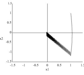
Fig. 1. Chattering effect.

Let us analyze the following unstable linear system:

Y(s)

1_

U(s)

" o r

.

x(0

"o"

1 x(t)= - 5 2 x(t)+ ^ u(t)

s(x) = [l l]x(t)

p5(k) = k + \

K = 10

The control action will be: - l

[1 1] [1 1]

0 1 - 5 2 x{t)-a

= - [ - 5 3]x(t) + a = 5x1(t)-3x2(t) + a

Thus the control action will be,

//s(x) < 0 thenu(t) = 5xi(t) - 3x2(t) + 10 7/s(x) = 0 thenu(t) = 5x1(t)-3x2(t) //s(x) > 0 thenu(t) = 5xi(t) - 3x2(t) - 10

(14)

(15)

Fig. 1 shows the chattering effect assuming that the simulation is carried out with a sampling time of 0.02 s.

Fig. 2 shows the temporal evolution of s(x). The mean square error is approximately 0.0195 when it is calculated from 0.2 s.

3. Chattering elimination

As mentioned before, the main drawback of SM control is the chattering problem resulted from the switching from one value to another. As it was observed in the previous example, the chattering problem comes from the fact that the behavior of s(x) in discrete implementations of the algorithm, is oscillatory from a certain time.

The origin of these oscillations is the discrete implementation of the system:

0 0.1 0.2 0.3 0.4 0.5 0.6 0.7 0.8 0.9 1 Time (s)

Fig. 2. Temporal evolution of s(x).

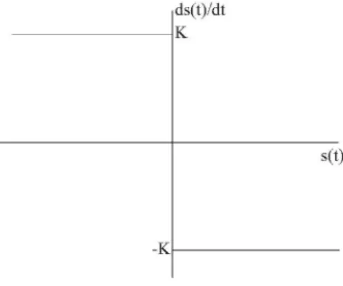
when it is controlled by

K ifs(t) < 0 V ( t ) :

-K ifs(t) > 0 (16)

Fig. 3 shows the phase plane of this system.

The discrete implementation of this system with zero order holding device and sampling time T corresponds to the system:

(17)

(18) K ifsk > 0

It can be shown that there is a limit cycle of amplitude Ai = 0.5KT and frequency a>i = TCJT, i.e. 2 samples per cycle. In order to over-come the chattering problem, a smooth transition is introduced between these two control actions. The resultant controller is a combination of the discontinuous one used to create the SM (ana-lyzed in the previous section) outside the layer and applying the equivalent control method inside this layer. Therefore, it is sug-gested in this work to switch from the SM control explained before to the equivalent control according to the position of the state tra-jectory.

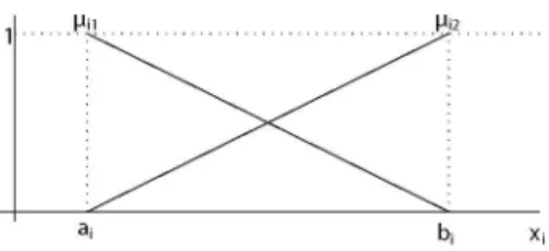
The solution proposed here for this problem is converting the VSC in FLC by defining two fuzzy sets for s(x) as shown in Fig. 4.

Ifs(x)isM- thens(x) = K

Ifs(x)isM+ thens(x) = -K

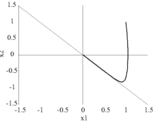
The phase plane of the system given in (1) is shown in Fig. 5

-phi phi s(t)

Fig. 4. Membership functions fors(x).

The necessary value of <P to avoid the limit cycle is

<P >AL >4Al = 2I<T. The resultant fuzzy VSC is:

Ifs(x)isM- then u(t) = -\SB(x(t))r\s(a0(x(t)) + A(x(t))x(t)) - K)

Ifs(x)isM+ then u(t) = -\S B(x(t))]-\S(a0(x(t)) + A(x(t))x(t)) + K) (19)

Thus, with this controller, the system is still verifying the fol-lowing switching condition given in (6)

Ifs(x) < 0 thens(x) > 0 Ifs(x) = 0 thens(x) = 0 Ifs(x) > 0 thens(x) < 0

(20)

so that it will still have a unique equilibrium point in x=0.

Example:

In the previous example, it can be clearly seen that s(x) oscillates with an amplitude of Ai = 0A, so it may be reasonable to choose 0 = 0.5. Now, the proposed FLC is applied for the same system in the previous example with the same sampling time and the fuzzy sets shown in Fig. 4 with <P = 0.5.

It can be clearly shown in Figs. 6 and 7 the effectiveness of the proposed controller in eliminating the chattering effect. The mean square error is 4.0650e-005 from 0.2 to 1 s.

Fig. 7 shows the smoothness obtained by applying the proposed controller.

In this paper, fuzzy inference is applied to switch from the discontinuous controller to the equivalent one by regarding the dis-tance from the switching hyperplane as a variable of the premise of the control laws.

4. Stability analysis

Firstly, consider the feedback system in (12) with a singular point in x = 0. It is fair enough for example that ao(0) = 0 to satisfy the following condition.

-K

ds(t)/dt

S(t)

1.5

1

0.5

3 0

-0.5

-1

-1.5

-1.5 -1 -0.5 0 0.5 1 1.5 xl

Fig. 6. Chattering elimination applying the proposed fuzzy algorithm.

xn(r)x = 0 = 0[ao(x(t)) +A(x(t))x(t) - bn(x)[SB(x(t))]-* x(S(a0(x(r))-M(x(r))x(r))-a)]x = 0

= a0(0) - BiOHSBiOM^SaoCO) = 0 (21)

Since s(x)=Sx = 0 is a stable linear dynamic system of reduced order, there should exist a Lyapunov function for this system [17,31]:

[xi x2 X n - l

Vr(x) = xJPrxr = xT

Pr 0

0 0

which should fulfill that Vr(x) is a positive definite function in xr and [dVr(x(r))]/dr is a negative definite one inxr.

Let us define the following Lyapunov function for the controlled system:

V(x) = Vr(x) + S(x)z

The two terms in Eq. (22) should verify:

Vr(x) > 0 Vx s mn

s(x)2 > 0 Vx s mn

(22)

(23)

J0 0.1 0.2 0.3 0.4 0.5 0.6 0.7 0.8 0.9 1

Time (s)

Fig. 7. Temporal evolution of s(x).

where V(x) should be at least a positive semidefinite function. More-over,

Vr(x0) = 0 ^ x o = [0---Oxn0r n 0 _ 0 -o- xn0 = 0 s ( x0)2= x2

V(x) = 0 # x = 0

Therefore, it is clear that V(x) is a positive definite function. The derivative of Lyapunov function becomes:

dV(x(t)) dVr(x(t)) + 2s(x)s(x) dt dt

The two terms in Eq. (25) should verify:

dVr{x{t))

dt < 0 Vx s SH"

(25)

(26) 2s(x)s(x) < 0 Vx s SH"

where (dV(x))jdt should be at least a negative semidefinite function. Moreover,

^ ° l = 0 ^ x 0 = [0...0 xn 0f

2s(x0)s(x0) = 2xn0a = 0 # x „0 = 0

dV{x)

~dT

(27)

where it is evident that dV{x)jdt is a negative definite function. Thus, the feedback system is an asymptotically stable one. Moreover,

V{x) is a positive definite Vx s SH"

dV(x) dt

and

is a negative definite Vx s SHn

(28)

V(x) -* ooas ||x|| -* oo

Therefore the system is a globally and asymptotically stable one.

5. Proposed controller (FLC-VSC)

There exist various techniques to design the FLC-VSC. In most of the works carried out in this field [12,24,41], the fuzzy system is described as follows:

x =A{x)x + B{x)u (29)

This means that the non linear fuzzy system is linearized with respect to the origin in each IF-THEN rule, which means that the consequent part of each rule is a linear function with zero affine term. This will in turn reduce the accuracy of approximating non linear systems. In this study, a design of FLC-VSC is presented based on T-S fuzzy model [32] taking into account the effect of the inde-pendent term in both the fuzzy system and controller.

The fuzzy system in this work is represented by the affine T-S fuzzy model.

x = a0(x) + A{x)x + B{x)u (30)

5.1. Fuzzy logic controller based variable structure controller (FLC-VSC)

Let the (ij . . . i„ )th rule of the T-S model be represented as: If this steady state value exists, the control action becomes,

S(J'i ~U) : ifXl isMj1 andx2 isM^... andxn isM^ thenx •. +y4(i'i-in)x + B(I'i-I'n)u

Jl'l-l'n)

where M*i (i'i = 1, 2 T\) are fuzzy sets for X\, M^ (i2 = 1, 2 r2) are fuzzy sets for x2, MJp (in = 1,2 r„) are fuzzy sets for x„. Therefore the complete fuzzy system has T\ X r2 x . . . r„ rules. The membership functions of the fuzzy system are overlapped by pairs. With this model, the model parameters can be identified using the algorithms developed by authors in [13,14].

The state vector is:

XT = [ Xi X2 . . . Xn]

of n dimension, and u is a scalar input. The vectors and matrices in these rules are described in a canonical controllable form:

nV-i-in) .

0

„ ( l ' l - l ' n ) J0

(32)

^ ( 1 ' l - i n ) . 0

0

0

a(U-..in)

4

1

0

0 1-in)

0

1

0

<fe

fa)

a[

0

0 1 1-in)

(33)

! ( l ' l - i n ) :

0

h ( i l - i n )

which is equivalent to be rewritten as:

x = a0(x)+A(x)x(t) + B(x)u

(34)

(35) where ao(x),A(x) and B(x) matrices are determined by the following fuzzy system:

(36) S(h ..^n) : ifxiisM^ andx2 isM%.. .andxnisM1^ then a0

= aiiJ['in)andA=A^- J") and B = B^'i • • -1'")

In conclusion, the new proposed method can be considered as a two level one: the first level includes the calculation of ao(x), A{x) and B(x) resulting matrices from the above identified fuzzy system and the second one is obtaining the control action mentioned above in (19):

Ifs(x)isM" thenu(t) = -[SB(x)]_1(S(a0(x) +A{x)x) -K)

Ifs(x)isM° thenu(t) = -[SB(x)]_1S(a0(x)+A(x)x) (37) Ifs(x)isM+ then u(t) =

6. Non-zero final state

-[SB(x)]-\S(a0(x)+A(x)x)+K)

The objective now is to approach a steady state xp. The first con-dition to impose is that there is an input signal up that allows the system:

x(t) = a0(x(t)) +A(x(t))x(t)+B(x(t)Mt) (38)

to maintain this steady state, i.e., the system should comply:

0 = a0 (xp) + A{xp )xp +B{xp)up (39)

u„

where B+(xp) is pseudoinverse. B + {xp) = {Bt *Bf1 *Bt

It can be observed that in this case:

1

'(Xp): 0 0 -bn(Xp)

If we change the variables in (38) as follows:

x ( t ) = xp +Ax(t) u(t) = up + Au(t)

Ax(t) = a0{x{t)) + A{x{t)){xp + Ax(t)) + B{x{t)){uv + Au(t))

we will obtain a new system:

Ax(t) = a0(x(t))+A(x(t))xp

+ B(x(t))up+A(x(t))Ax(t) + B(x(t))Au(t)

This means that:

Ax(t) = ap0(x(t))+A(x(t))Ax(t) + B(x(t))Au(t)) where

apoMO) = ao(x(t)) +A(x{t))xp + B{x{t))up

It will satisfy in this new system (44) that,

Ax = 0 =>• x = Xp

apo(xp) = a0{xp) +A{xp)xp+B{xp)uv = 0

(41)

(42)

(43)

(44)

(45)

(46) This means that the required condition is satisfied so that the VSC control:

Ifs(Ax) < 0 then u(t) = -\SB(x(t))r\S(apo(x(t)) + A(x)Ax(t)) - K)

Ifs(Ax) = 0 thenu(t)=-[SB(x(t))l-1S(ap 0(x(t))+/l(x)Ax(t)) ( 4 7 ) Ifs(Ax) > 0 thenu(t)=-lSB(x(t))r\S(ap0(x(t)) + A(x)Ax(t)) + K)

results in a feedback system asymptotically and globally stable in:

Ax = 0 =>• x = Xp

Au(t) = -[SBMO)]-1 (S(ap0(x(t)) + A(x(t))Ax(t)) - a)

u(t) = up- [ S B M ^ r ^ a o M O H A M t ^ X p +B(x(t))up + A(x(t))Ax(t)) -a) = up- [SB(x(t))]-*SB(x(t))up

- [SBCx(t))]-1 (S(a0(x(t))+A(x(t))xp +A(x(t))Ax(t)) - a) = -[SB(x(t))]-1(S(a0(x(t))+A(x(t))Xp

+A(x(t))(x(t)-Xp))-a) = -[SB(x(t))r1(S(a0(x(t))

+ A(x(t))x(t))-a) (48)

Therefore, it is not necessary to know the value of up explicitly. Finally, the controller becomes:

Ifs(Ax) < 0 then u(t) = -[SB(x(t))]_1(S(a0(x(t)) + A(x(t))x(t)) - K)

7. Estimation of fuzzy T-S model's parameters

T-S model [32] is based on estimating the nonlinear sys-tem parameters minimizing a quadratic performance index. The method is based on the identification of functions of the following form:

/:!«"

y = / ( x1, x2, . . . , xn)

Each IF-THEN rule for an nth order system can be written as follows:

5(11 -in) • jfXl ,sjvfii a n cj _ _ _Xn isf^- theny = p$-I'n)

+ pa i . . i n )X 2 + . . .+ p( l1. . . i n )X n

where the fuzzy estimation of the output is:

(50)

£^r--£ti

"

w

+P('1-'..>X1

p^i • • • % + . . . + P -(l'l-in)v

E L i - E L i ^ - ' - ^ x )

(51)

where

n

( l

^

(x) = J]/A

,(x,)

1=1

w

being /AJ,\(XJ) the membership function that corresponds to the fuzzy set Mi.

Let {x\k,X2k< • • ->xnk>yk} be a set of input/output system sam-ples. The parameters of the fuzzy system can be calculated as a result of minimizing a quadratic performance index:

J

,(y

-9kf = \\y-xp\\

k =1

Y=[y\ yi ••• ym]

p

[ # • • » # • • • » $ • • • » .

„(ri-.rn) (ri...rn)

p(l...D 1

(52)

(53)

ft -

r

"\.. ft^x

nl

Pni" An xlm- • -A

o(ri...rn) otiv-.rn)

fm - - •A'm

( 1 - D v •^nm and

^,...w

E ^ i - E t i ^ - ' ^ C x f c )

(54)

If X is a matrix of full rank, the solution is obtained as follows:

J = \\Y-XP\\2 = (Y -XP)J(Y -XP)

VJ = XT(Y - XP) = XTY - XTXP = 0 P = (XTXTlXTY

(55)

Fig. 8. Membership functions of the fuzzy system.

Fig. 9. One link robot.

8. Restrictions of T-S identification method

The validity of the control design depends mainly on the mod-eling accuracy of the controlled system and the proposed method offers a great accuracy. On the other hand, to make the procedure practical, the modeling stage must be computationally efficient. Modeling phase is fundamental both in the analysis process of a dynamic system and the design of a control system. The method proposed in [32] arises serious problems as it can not be applied in the most common case where the MFs are those shown in Fig. 8.

The MFs fin(xi) = (bi-xi)l(bi-ai) and /ia(x,) = (x,--a,)/(b,--a,) are defined in an interval [a,-, b{\ which should verify:

Mn(Oi) = l Vn(bi) = 0

fii2(Oi) = 0 jii2{bi) = \

Mil(Xi) + Mi2(Xi) = l

For this case which is widely used, it can be easily demonstrated [13,14] that the matrixXis not of full rank and therefore XTX is not invertible, which makes the mentioned method of T-S invalid.

The solution proposed in [32] avoids the occurrence of this sit-uation. It can be clearly seen in [32] that when the matrix X is of full rank and the T-S method is applicable where the authors find the optimum MFs when they are non overlapping ones, minimiz-ing the performance index and reducminimiz-ing the problem to a nonlinear programming one. In [14], a detailed proof shows that T-S method is restricted and invalid when the MFs are overlapped by pairs.

The authors developed an approach [ 1 ] which can be considered as a generalized version of T-S method with optimized performance in approximating (locally and globally) nonlinear functions. It is a simple approach with few computational effort, based on the well known parameters weighting method for tuning T-S parameters to improve the choice of the performance index and minimize it.

9. Illustrative example

Example 9.1. One link robot

Consider the problem of estimating a one link robot manipulator (see Fig. 9) using the above mentioned estimation methods.

0 45 90 135 180 6(deg.)

Fig. 10. Membership functions for the angle x of the one link robot.

where mi is the mass at the end of the link, l\ is the length of the link, g\ is the gravitation constant, 6\ is the angle of link with respect to its null position, l\ is the moment of inertia; with

m-i = 2 kg, h = 1 m, lcl = 0.5 m, h = 0.25 kgm2, and /3i = 0.05 N/m/s. This system can be rewritten in state space form as follows:

X\ = 9i

x

= e

x\

X2

=

x

-W\x

+g\)

+

H i

-*\

s{x) = [2 l ] x ( 0

p(k) = k + 2, k = 5

Firstly, the model of the one link robot is estimated in five operation points for the angle and three operation points for its derivative. The universe of discourse of the angle is [0, n] and the one of the angular velocity is [- 1,1]. Both MFs for the angle x and its derivative x are shown in Figs. 10 and 11 respectively.

If we apply the T-S method directly to this example, then the condition number of the matrix X is 3.4148e + 015, which shows clearly a non reliable result. Using the parameters' weighting method with weighting factor )/ = 0.01, the robot fuzzy model can be represented as follows:

Su: If x1 is M\ and x2 is M\ then

x2 = 0.3445 - 9.1813XJ - 0.1974x2 + 0.9998u S1'2: Ifxi isMj andx2 isM2 then

x2 = -9.3391X! - 0.2042x2 + 0.9999u S1 3: Ifxi isMj andx2 isM3 then

x2 = -0.2534 - 9.5255X! - 0.1963x2 + 0.9997u S2'1: If Xi is M2 and x2 is M\ then

x2 = -0.5969 - 7.631 lX! - 0.1489x2 + 1.0002u S2'2: If X! is M2 and x2 is M2 then

x2 = -0.8261 - 7.7832X! - 0.1466x2 + 0.9999u

0 0.5 1 1.5 2 2.5 3 3.5 4 4.5 Time (seconds)

Fig. 12. Transient response of the one-link robot.

S2 3: If x2

S3-U.U

x2

S3 2: If x2

S3 3: If x2

S4'1: If x2

S4'2:If x2

S4 3: If x2

S5 1: I f x2

S5'2: If x2 =

S5 3: I f x2

Xi is M2 and x2 is M | 1.04457.9457x1 -Xi is M3 and x2 is M\ 2.76274.2486x1 -Xi is M3 and x2 is M2 2.95054.3735x1 -Xi is M3 and x2 is M3

3.08964.5363x1 -Xi is M4 and x2 is M\ 4.51360.8475x1 -Xi is M4 and x2 is M2 4.65460.9693x1 -Xi is M4 and x2 is M | 4.72341.1231x1 -Xi is M\ and x2 is M\ 1.8201+0.7473x1 -Xi is M\ and x2 is M2 1.7920 + 0.5847x1 -Xi is M\ and x2 is M | 1.8702 + 0.4526x1

-then 0.1521x2 + l then 0.1119x2 + 0 then 0.1090x2 + l then 0.1060x2 + 0 then 0.0736x2 + 1 then 0.0690x2 + 0 then 0.0672x2 + 1 then 0.0295x2 + 1 then 0.0138x2 + l then 0.0067x2 + 0

.OOOlu

9998u

.OOOlu

9999u

,0002u

9999u

,0002u

.OOOOu

.OOOlu

,9998u

The resultant mean square error from this approximation is 1.5367e-004.

As it can be observed, the results obtained through the param-eters' weighting method are always better than with the original T-S method. The transient response is shown in Fig. 12.

Now, the proposed FLC is applied for the same system in the previous example with the same sampling time and the fuzzy sets shown in Fig. 13 with <P = 1.

It can be clearly shown in Fig. 14 the effectiveness of the pro-posed controller in eliminating the chattering effect. The transient

40 60 80 100 Angle (deg.)

Fig. 17. Phase plane of the robot link from the origin to a non zero final state with

the proposed control algorithm developed for chattering elimination. 60 80 100 120 140

Angle (degrees)

Fig. 14. Chattering elimination.

140 120 100

Fig. 18. Transient response of the robot link subjected to a step input and a load of

0.5 kg in the end effector. 0 0.5 1 1.5 2 2.5 3 3.5 4 4.5 5

Time (seconds)

Fig. 15. Transient response of the one-link robot.

response is shown in Fig. 15.The temporal evolution of s(x) is shown in Fig. 16.

The results obtained show that the system is stabilized by apply-ing the proposed FLC-VSC. Fig. 17 shows the phase plane of the robot link from the origin to a non zero final state with the proposed control algorithm developed for chattering elimination. Fig. 18 shows the transient response of the robot link controlled by the proposed FLC-VSC controller subjected to a step input and to a load in the end effector of a mass of 0.5 kg. The position steady state error is 0.0146° and the velocity steady state error is 0.0000e-004°/s. To examine the robustness of the proposed controller, the system

Fig. 19. Transient response of the robot link subjected to disturbances.

0 0.5 1 1.5 2 2.5 3 3.5 4 Time (seconds)

Fig. 16. Temporal evolution of s(x).

4.5

Fig. 20. Transient response of the robot link controlled by the FLC-VSC subjected to

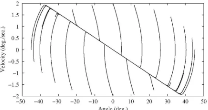
2 1.5 1 0.5 0 -0.5 -1 -1.5 -2

-10 0 10 Angle (deg.)

Fig. 21. Trajectories of the states of the system for several initial conditions.

has been subjected to successive disturbance effects of 5°, -3° and 9° with respect to its equilibrium state as shown in Fig. 19. It is clearly shown that the robot link returns rapidly and smoothly to its equilibrium condition after each disturbance. Moreover, we have proven that the FLC-VSC is robust and invariant against mea-surement noise. If we suppose that the angle sensor introduces a noise of a= 1°, it can be observed that the output is only affected by

a = 0.0870° as shown in Fig. 20. Fig. 21 shows several trajectories of the system for several initial conditions.

10. Conclusion

Due to the similarity between FLC and VSC, a design of a non linear controller based on both techniques has been presented. The fuzzy system and controller have been represented by Affine T-S model. The main contribution of this work is that firstly new functions for chattering elimination and error convergence without sacrificing invariant properties are proposed which is considered the main drawback of the VSC control. Secondly, the global stability of the controlled system is guaranteed within the valid range of the T-S identification. The robustness of any control design depends mainly on the modeling accuracy of the controlled system. The main problem encountered in modeling T-S model is that it cannot be applied when the MFs are overlapped by pairs.

An optimization estimation approach has been used to improve the local and global approximation and modeling capability of T-S identification methodology. The parameters' weighting optimiza-tion method has been applied to reduce the error between the original system and the identified one.

A one link robot is chosen as a nonlinear unstable system to eval-uate the robustness, effectiveness and remarkable performance of optimization approach and the high accuracy obtained in approx-imating nonlinear systems in comparison with the original T-S model. Simulation results indicate the potential and generality of the algorithm. In this paper, we prove that these algorithms con-verge very fast, thereby making them very practical to use. The application of the proposed FLC-VSC shows that both alleviation of chattering and robust performance are achieved with the proposed FLC-VSC controller. The effectiveness of the proposed controller is proven infront of disturbances and noise effects.

References

[1] B.M. Al-Hadithi, A. Jimenez, F. Matia, A new approach to fuzzy estimation of Takagi-Sugeno model and its applications to optimal control for nonlinear systems, Applied Soft Computing 12(1) (January 2012) 280-290.

[2] J.M. Andujar, A.J. Barragan, A methodology to design stable nonlinear fuzzy

control systems, Fuzzy Sets and Systems 154 (September (2)) (2005) 157-181.

[3] J.M. Andujar, A.J. Barragan, A general and formal methodology for designing

stable nonlinear fuzzy control systems, IEEE Transactions on Fuzzy Systems 17 (October (5)) (2009) 1081-1091.

A. Cavallo, High-order fuzzy sliding manifold control, Fuzzy Sets Systems 156 (2005) 249-266.

B. Chen, X. Liu, S. Tong, Adaptive fuzzy output tracking control of MIMO non-linear uncertain systems, IEEE Transactions on Fuzzy Systems 15 (April (2)) (2007) 287-300.

F. Gang, A survey on analysis and design of model-based fuzzy control systems, IEEE Transactions on Fuzzy Systems 14 (October (5)) (2006) 676-697. S.-J. Huang, W.-C. Lin, Adaptive fuzzy controller with sliding surface forvehicle suspension control, IEEE Transactions on Fuzzy Systems 11 (August (4)) (2003) 550-559.

C. Hua, G.D. Xinping Guan, Variable structure adaptive fuzzy control for a class of nonlinear time-delay systems, Fuzzy Sets and Systems 148 (2004) 453-468.

C.-L. Hwang, A novel Takagi-Sugeno-based robust adaptive fuzzy sliding-mode controller, IEEE Transactions on Fuzzy Systems 12 (October (5)) (2004) 676-687.

C.-L. Hwang, C.Jan, Optimal and reinforced robustness designs of fuzzy variable structure tracking control for a piezoelectric actuator system, IEEETransactions on Fuzzy Systems 11 (August (4)) (2003) 507-517.

C.-L. Hwang, H.-Y. Lin, A fuzzy decentralized variable structure tracking control with optimal and improved robustness designs: theory and applications, IEEE Transactions on Fuzzy Systems 12 (October (5)) (2004) 615-630.

S. Jacob, J. Munighan, Designing fuzzy controllers from a variable struc-ture standpoint, IEEE Transactions on Fuzzy Systems 5 (February (1)) (1997) 138-144.

A. Jimenez, B.M. Al-Hadithi, F. Matia, An optimal T-S model for the estimation and identification of nonlinear functions, WSEAS Transactions on Systems and Control 3 (October (10)) (2008) 897-906.

A. Jimenez, B.M. Al-Hadithi, F. Matia, Improvement of Takagi-Sugeno fuzzy model for the estimation of nonlinear functions, Asian Journal of Control 14 (November(6)) (2012) 1-15, http://dx.doi.org/10.1002/asjc.310.

TAJohansen, R. Shorten, R. Murray-Smith, On the interpretation and identifi-cation of dynamic Takagi-Sugeno models, IEEE Transactions on Fuzzy Systems 8 Qune (3)) (2000) 297-313.

K. Jae-Hun, C.-H. Hyun, E. Kim, M. Park, New adaptive synchronization of uncer-tain chaotic systems based on T-S fuzzy model, IEEE Transactions on Fuzzy Systems 15 Qune (3)) (2007) 359-369.

H. Khalil, Nonlinear Systems, Prentice Hall, 2002, ISBN 0-13-067389-7. LT. Koczy, It Hirota, Size reduction by interpolation in fuzzy rule bases, IEEE Transactions on Systems, Man, and Cybernetics, Part B: Cybernetics 27 (February (1)) (1997) 14-25.

C.-C. Kung, T.-H. Chen, Observer-based indirect adaptive fuzzy sliding mode control with state variable filters for unknown nonlinear dynamical systems, Fuzzy Sets and Systems 155 (2005) 292-308.

H.K. Lam, F.H. Leung, Fuzzy rule-based combination of linear and switching state-feedback controllers, Fuzzy Sets Systems 156 (2005) 153-184. K.-Y. Lian,C.-H.Su,C.-S. Huang, Performance enhancement for T-S fuzzy control using neural networks, IEEE Transactions on Fuzzy Systems 14 (October (5)) (2006)619-627.

C.-Y. Liang, J.-P. Su, A new approach to the design of a fuzzy sliding mode controller, Fuzzy Sets and Systems 139 (2003) 111-124.

J.-C. Lo, Y.-H. Kuo, Decoupled fuzzy sliding-mode control, IEEETransactions on Fuzzy Systems 6 (August (3)) (1998) 426-435.

F. Matia, B.M. Al-Hadithi, A. Jimenez, P.S. Segundo, An affine fuzzy model with local and global interpretations, Applied Soft Computing (September (6)) (2011)4226-4235.

J.A. Meda-Campana, B. Castillo-Toledo, On the output regulation for TS fuzzy models using sliding modes, in: Proc. Amer. Control Conf., Portland, OR, 2005, pp. 4062-4067.

D. Simon, Design and rule base reduction of a fuzzy filter for the estimation of motor currents, International Journal of Approximate Reasoning 25 (2000) 145-167.

D. Simon, Training Fuzzy Systems with the Extended Kalman Filter, Fuzzy Sets and Systems 132 (2002) 189-199.

I. Skrjanc, S. Blazic, O. Agamennoni, Interval fuzzy model identification using l-Norm, IEEE Transactions on Fuzzy Systems 13 (October (5)) (2005). J-J.E. Slotine, Applied Nonlinear Systems, Prentice-Hall, Englewood Cliffs, NJ, 1991.

T. Takagi, M. Sugeno, Fuzzy identification of systems and its applications to modeling and control, IEEE Transactions on Systems, Man, and Cybernetics SMC-15(1) (1985) 116-132.

K. Tanaka, H.O. Wang, Fuzzy Control Systems Design and Analysis: A Linear Matrix Inequality Approach, Wiley, New York, 2001.

C. Tao, J. Taur, Design of Fuzzy Controllers with Adaptive Rule Insertion, IEEE Transactions on Systems, Man, and Cybernetics—Part B: Cybernetics 29 (1999) 389-397.

J.S. Taur, C.W. Tao, L.M. Chan, Adaptive fuzzy terminal sliding mode controller for linear systems with mismatched time-varying uncertainties, IEEE Trans-actions on Systems, Man, and Cybernetics—Part B: Cybernetics 34 (1) (2004) 255-262.

[38] L. Tzuu-Hseng, T.Shun-Hung, Fuzzy bilinear model and fuzzy controller design for a class of nonlinear systems, IEEE Transactions on Fuzzy Systems 15 (June (3)) (2007) 494-506.

[39] V.A. Utkin, Sliding Modes and Their Applications invariable Structure Systems, Nauka, Moscow, 1978 (in Russian, also Moscow: Mir, 1978, in English).

[40] L. Wang, J. Mendel, Back-propagation of Fuzzy systems as nonlinear dynamic

system identifiers, in: IEEE International Conference on Fuzzy Systems, San Diego, CA, 1992, pp. 1409-1418.

[41] J.C. Wu, T.S. Liu, A sliding-mode approach to fuzzy control design,

IEEE Transactions on Control Systems Technology 4 (March (2)) (1996) 141-151.