energies
Article
Probability Model Based Energy Efficient and
Reliable Topology Control Algorithm
Ning Li *, Jose-Fernan Martinez-Ortega, Lourdes Lopez Santidrian and Juan Manuel Meneses Chaus
Research Center on Software Technologies and Multimedia Systems for Sustainability (CITSEM), Universidad Politécnica de Madrid (UPM), Madrid 28031, Spain; [email protected] (J.-F.M.-O.); [email protected] (L.L.S.); [email protected] (J.M.M.C.)
* Correspondence: [email protected]; Tel.: +34-688-500-639
Academic Editor: Robert Lundmark
Received: 20 June 2016; Accepted: 12 October 2016; Published: 20 October 2016
Abstract: Topology control is an effective method for improving the performance of wireless sensor networks (WSNs). Many topology control algorithms can achieve high energy efficiency by dynamically changing the transmission range of nodes. However, these algorithms prefer to choose short multihop communication links rather than the long directly communication links which also energy efficient probabilistic. Note that these fact, in this paper, we propose a mathematic model to explore the probability that the long directly communication links are more energy efficient than the short links. We investigate the properties of this probability and find out the optimal transmission range which has highest probability of energy efficient. Based on this conclusion, we propose the
energy efficient and reliable topology control algorithm (ERTC) to maintain ther-range for the nodes
instead of thek-connection; moreover, ERTC can achieve energy efficient and network connection at
the same time.
Keywords:wireless sensor network (WSN); topology control; energy efficient; reliable
1. Introduction
Wireless sensor networks (WSNs) have become more and more widely used and important in recent years. The properties of WSNs—which contain hundreds or thousands of sensors—are limited by the energy, the bandwidth, the capability of computing, etc. Moreover, in most applications, the WSNs are arranged in the remote area where changing the sensor nodes always impossible or inconvenient, so how to save the node energy and prolong the network lifetime is important for WSN. There are many algorithms have been proposed to improve the network reliable and energy efficient for WSN. One remarkable approach is topology control. Topology control has been proposed to address many problems in WSNs by adding or deleting nodes/links according to certain algorithms. The aim of topology control is to reduce energy consumption and preserve other fundamental properties for
the network at the same time [1], such as network connectivity, reliability, fault-tolerant, coverage, etc.
In WSNs, topology control can be implemented in three approaches [2]: (1) Power Adjustment
Approach: minimizing the transmission power by adjusting the transmission range of node; in this approach, the long distance communication links will be eliminated while the short links will be chosen; (2) Power Model Management: controlling the feature of the operating mode to reduce energy consumption; there are four operating modes: sleep mode, idle mode, transmission mode, and receiving mode; since the energy consumption during the transmission mode and receiving
mode is generally higher than that in the sleep mode [3], so switching the redundant nodes into
sleep mode can save energy obviously [4]; (3) Clustering Approach [5]: selecting a set of nodes
in the network to construct an efficiently hierarchical topology; the clusterheads are restricted to
Energies2016,9, 841 2 of 17
certain tasks like collecting data, processing packets, or forwarding packets to non-clusterheads; the non-clusterheads nodes collect data and transmit the data packets to the clusterheads. In this paper, we mainly concentrate on the first one, i.e., the power adjustment approach.
To the power adjustment approach, on one hand, for reducing interference and energy
consumption, each node transmits packets with relative low power [6]. The algorithms are generally
localized, i.e., each node uses only the information that is one or two hops away. The problem of minimizing the total energy consumption for the whole network is NP-hard in both two and three
dimensional space [7,8]. In addition, if the WSN consists thousands of nodes, it is difficult to calculate
the optimal transmission ranges for transmitting the packets to the concerned nodes [3]. On the other
hand, even reducing the transmission range of nodes is the most common and effective approach to control the network topology and reduce the energy consumption in WSN, but in this paper we will show that the long directly communication links can probabilistically spend less energy than the short indirectly communication links, i.e., it is probabilistic when reducing the energy consumption of network by reducing transmission range.
Motivated by these, in this paper, we explore the probability of reducing energy consumption by reducing the transmission range, and investigate the properties of this probability under different scenarios. Based on the conclusions, we propose an energy efficient and reliable topology control algorithm (ERTC) which meets the requirements of network connection and energy efficient at the same time. The contributions of this paper are as follows:
• we propose a mathematic probability model for energy consumption analysis when applying
the transmission power adjustment approach. To the best of our knowledge, this is the first probability analysis model for this kind of issue;
• we analyze the probability model in detail and explore the features of this model under different
network parameters;
• we propose an ERTC based on these conclusions, which maintain ther-range of the node instead
of thek-connection and can adapt the network dynamic.
The rest parts of the paper are organization as follows: in Section2, we will introduce the related
works of the and topology control; Section3will provide the network model and state the problems
which will be investigated in this paper; we will introduce the probability model and analysis the
properties of this model in Section 4; in Section 5, we will introduce the ERTC method in detail;
Section6explores the performance of ERTC based on simulation; in Section7, we conclude this paper.
2. Related Works
The latest surveys of network topology control algorithms can be found in [2,9–11]. The primary
goals of topology control are to guarantee the network connection and reduce the energy consumption as far as possible. Many heuristic algorithms have been proposed, such as, Local Minimum Spanning
Tree (LMST) [12], Local Tree-based Reliable Topology (LTRT) [6], A1 [13], Poly [14], Centralized Robust
Topology Control Algorithm (CRTCA) [15], Cooperative topology control scheme with Opportunistic
Interference Cancelation (COIC) [16], Local Mean Neighbor (LMN) [17], Local Mean Algorithm
(LMA) [17], Smart Boundary Yao Gabriel Graph (SBYaoGG) [18], BRASP [19], etc. Almost all of
these protocols regard topology control as a technique in which nodes dynamically change their
transmission ranges to gain energy efficient and network connection. In [12], each node builds its
own LMST independently and only on-tree nodes that one-hop away are kept in the final topology. Considering the fact that the LMST always constructs one-connected network in the final topology,
in [6], the authors propose LTRT algorithm, which combines the idea of LMST and Tree-based Reliable
Topology (TRT) together to guaranteek-edge connectivity in the resulting topology. LTRT can maintain
the network connection at low computational cost and energy consumption. In [19], due to the lossy
Energies2016,9, 841 3 of 17
reachability. The authors explore the minimal transmission power for each node when the network reachability is above a given threshold. Based on the conclusion, the authors propose BRASP algorithm to improve the energy efficiency and reduce the average node degree. A1 assumes the network topology as a connected network and finds a set of active nodes to form connected dominating set
(CDS) [13]. This algorithm can form a reduced topology while keeping the network connection and
coverage at the same time. In addition, A1 forms the CDS which comprising high energy nodes in a single phase construction process and a set of active nodes for energy efficiency and better sensing
coverage, respectively. Similarly with A1, Poly [14] is also the algorithm based on CDS. In Poly,
the network is modeled as a connected graph. The protocol can turn off the unnecessary node and keep the network connection and coverage at the same time. LMN and LMA are the two typical
power adjustment topology control algorithms [17]. In LMA, all the nodes can get their node degree.
The algorithm sets the minimum threshold and maximum threshold for this number; if the node degree is less than the minimum threshold, the transmission range will be increased; otherwise, transmission range will be reduced. The principle of LMN is similar with LMA, but LMN does not set the maximum and minimum thresholds for the node degree. In LMN, the nodes use the mean neighbors’ node degree as the threshold to adjust the transmission ranges.
3. Network Model and Problem Statement
In general, there are three models can express the connection mode between nodes, which are
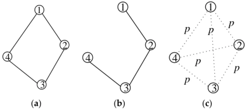
shown in Figure1[20]. Figure1a illustrates theknearest neighbor model; each node in this model has
constant node degree and maintains the node degree by changing communication range dynamically.
Figure1b illustrates the disc model; in this model, the transmission range is modeled as a disk with
radiusr; the nodes connect with other nodes that fall into its communication range. Figure1c illustrates
the Erdos-Renyi random graph that connects any two nodes by the same probability which is not
appropriate in WSNs. Disc model is more plausible in WSN since obtainingkneighbors is not always
feasible due to the communication range limitation [20]. Therefore, in this paper, we only interested
in the Disc model. The nodes in this model are uniform distributed and fixed; moreover, the nodes have different initial transmission ranges and can change their transmission ranges from zero to the maximum.
Energies 2016, 9, 841 3 of 17
transmission power for each node when the network reachability is above a given threshold. Based on the conclusion, the authors propose BRASP algorithm to improve the energy efficiency and reduce the average node degree. A1 assumes the network topology as a connected network and finds a set of active nodes to form connected dominating set (CDS) [13]. This algorithm can form a reduced topology while keeping the network connection and coverage at the same time. In addition, A1 forms the CDS which comprising high energy nodes in a single phase construction process and a set of active nodes for energy efficiency and better sensing coverage, respectively. Similarly with A1, Poly [14] is also the algorithm based on CDS. In Poly, the network is modeled as a connected graph. The protocol can turn off the unnecessary node and keep the network connection and coverage at the same time. LMN and LMA are the two typical power adjustment topology control algorithms [17]. In LMA, all the nodes can get their node degree. The algorithm sets the minimum threshold and maximum threshold for this number; if the node degree is less than the minimum threshold, the transmission range will be increased; otherwise, transmission range will be reduced. The principle of LMN is similar with LMA, but LMN does not set the maximum and minimum thresholds for the node degree. In LMN, the nodes use the mean neighbors’ node degree as the threshold to adjust the transmission ranges.
3. Network Model and Problem Statement
In general, there are three models can express the connection mode between nodes, which are shown in Figure 1 [20]. Figure 1a illustrates the k nearest neighbor model; each node in this model has constant node degree and maintains the node degree by changing communication range dynamically. Figure 1b illustrates the disc model; in this model, the transmission range is modeled as a disk with radius r; the nodes connect with other nodes that fall into its communication range. Figure 1c illustrates the Erdos-Renyi random graph that connects any two nodes by the same probability which is not appropriate in WSNs. Disc model is more plausible in WSN since obtaining k neighbors is not always feasible due to the communication range limitation [20]. Therefore, in this paper, we only interested in the Disc model. The nodes in this model are uniform distributed and fixed; moreover, the nodes have different initial transmission ranges and can change their transmission ranges from zero to the maximum.
1
2
3
4
1
2
3
4
1
2
3
4
p
p
p
p
p
p
(a) (b) (c)
Figure 1. Different network models: (a) k nearest neighbor model; (b) disc model; and (c) Erdos-Renyi random graph.
The notations and network definitions used in this paper are as follows:
n
The node number of the whole network;r The Euclidean distance between two nodes u and v, in this paper, we also use r to represent the initial transmission range;
The distance-power gradient;uv
P
The energy required to transmit data from node u to node v; The probability of energy efficient when applying the power adjustment topology control algorithm. Figure 1.Different network models: (a)knearest neighbor model; (b) disc model; and (c) Erdos-Renyi random graph.
The notations and network definitions used in this paper are as follows:
n The node number of the whole network;
r The Euclidean distance between two nodesuandv, in this paper, we also userto represent the
initial transmission range;
γ The distance-power gradient;
Puv The energy required to transmit data from nodeuto nodev;
Energies2016,9, 841 4 of 17
Definition 1. The communication range of node u is defined as the area where other nodes can receive u’s packet correctly.
In this paper, the communication ranges of nodes are circles, but may not be the same. Moreover, the transmission range can be changed from zero to maximum.
Definition 2.The energy Puvrequired to transmit data packet from node u to node v is defined as rγ, where r is the Euclidean distance between node u and node v, andγis a constant called the distance-power gradient whose typical value is between 2 and 4 [21–23].
Definition 3.The neighbors of node u are defined as the nodes which can receive the packet from node u and can reply message to node u.
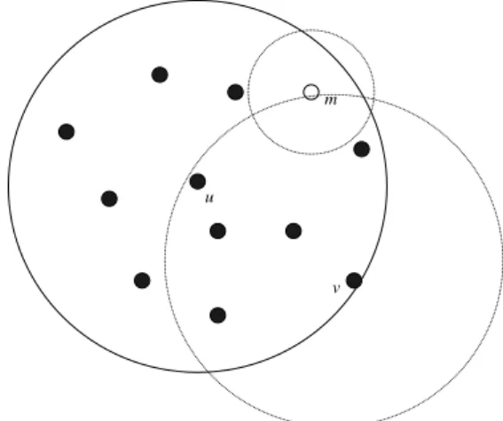
Consequently, as shown in Figure2, according to the definition of the neighbors, if nodevis
the neighbor of nodeu, then the nodeuis also the neighbor of nodev. In Figure2, even the nodem
locates in the communication range of nodeu, but it can not send packet to nodeudue to the small
transmission range, so nodemis not the neighbor of nodeu. Nodevis the neighbor node of nodeu,
since nodeualso locates in the transmission range of nodev.
Energies 2016, 9, 841 4 of 17
Definition 1. The communication range of node u is defined as the area where other nodes can receive u’s packet correctly.
In this paper, the communication ranges of nodes are circles, but may not be the same. Moreover, the transmission range can be changed from zero to maximum.
Definition 2.The energy
P
uv required to transmit data packet from node u to node v is defined asr
, where r is the Euclidean distance between node u and node v, and γ is a constant called the distance-power gradient whose typical value is between 2 and 4 [21–23].
Definition 3.The neighbors of node u are defined as the nodes which can receive the packet from node u and can reply message to node u.
Consequently, as shown in Figure 2, according to the definition of the neighbors, if node v is the neighbor of node u, then the node u is also the neighbor of node v. In Figure 2, even the node m locates in the communication range of node u, but it can not send packet to node u due to the small transmission range, so node m is not the neighbor of node u. Node v is the neighbor node of node u, since node u also locates in the transmission range of node v.
m
u
v
Figure 2. Definition of communication range and neighbor.
Definition 4.r-range of the node is defined as the optimal transmission range which has high probability of energy efficient.
Like the definition of k-connection for the network reliability and considering the probability that reduce the energy consumption by reducing the transmission range, if the nodes can maintain the optimal transmission range, i.e., r-range, the probability of energy efficient will be high.
As discussed in Section 2, many energy efficient topology control algorithms change the transmission range dynamically to gain energy efficient, but they fail to give the strict proof of whether this approach always effective or not; if not, what is the probability of this issue, and how to improve this probability? In this paper, we will analyze these issues in detail.
4. Probability Analysis
Theorem 1. After the transmission range adjustment, the probability that the energy consumption is less
than the previous one is
1
2 0
2
( ) 1
r
r x dx
r
.Proof. In WSN, supposing that node v is the neighbor of node u. when node u transmits packet to node v, the energy consumption is related to the distance between two nodes, which can be expressed as:
1 uv
P
r
, (1)Figure 2.Definition of communication range and neighbor.
Definition 4.r-range of the node is defined as the optimal transmission range which has high probability of energy efficient.
Like the definition ofk-connection for the network reliability and considering the probability that
reduce the energy consumption by reducing the transmission range, if the nodes can maintain the
optimal transmission range, i.e.,r-range, the probability of energy efficient will be high.
As discussed in Section 2, many energy efficient topology control algorithms change the
transmission range dynamically to gain energy efficient, but they fail to give the strict proof of whether this approach always effective or not; if not, what is the probability of this issue, and how to improve this probability? In this paper, we will analyze these issues in detail.
4. Probability Analysis
Theorem 1.After the transmission range adjustment, the probability that the energy consumption is less than the previous one isρ= r22
Rr
0(r
γ−xγ)γ1dx−1.
Proof.In WSN, supposing that nodevis the neighbor of nodeu. when nodeutransmits packet to node
v, the energy consumption is related to the distance between two nodes, which can be expressed as:
Energies2016,9, 841 5 of 17
whereris the Euclidean distance between nodeuand nodev,γis the distance-power gradient that
depending on the characteristics of the communication medium (2 ≤ γ ≤ 4, γ ≥ 2 for outdoor
propagation modes [23]);Puv1is the power needed for link between nodeuand nodev.
If the transmission ranges of nodeu and nodevare reduced based on the topology control
algorithm, then node u and node v cannot communicate directly, which is shown in Figure 3.
As a result, noden will be chosen as the relay node, where node n is the neighbor of both node
uand nodev. Thus, the energy needed to transmit packets from nodeuto nodevwill be:
Puv2∝r1γ+r2γ, (2)
wherer1is the Euclidean distance between nodeuand noden,r2is the Euclidean distance between
nodenand nodev;Puv2is the power needed for communicating between nodeuand nodevby using
relay noden.
Energies 2016, 9, 841 5 of 17
where r is the Euclidean distance between node u and node v, is the distance-power gradient that depending on the characteristics of the communication medium (2 4, 2 for outdoor propagation modes [23]); Puv1 is the power needed for link between node u and node v.
If the transmission ranges of node u and node v are reduced based on the topology control
algorithm, then node u and node v cannot communicate directly, which is shown in Figure 3. As a
result, node n will be chosen as the relay node, where node n is the neighbor of both node u and node v. Thus, the energy needed to transmit packets from node u to node v will be:
2 1 2
uv
P r r, (2)
where r1 is the Euclidean distance between node u and node n, r2 is the Euclidean distance between node n and node v; Puv2 is the power needed for communicating between node u and node v by using relay node n.
Figure 3. Transmission range adjustment.
Therefore, the issues we need to solve are when Puv2 is smaller than Puv1 and what is the probability that Puv2 smaller than Puv1. For exploring these issues, we define the Energy efficient Dominating Sets (EDS) as follows:
1 2
1 2
1
2
0 0
uv uv
P P
r r r
r r
r r
, (3)
where the first constraint means the energy consumption after power adjustment is smaller than the previous one; the second constraint make sure node u still can communication with node v by using a relay node; the third and the fourth constraints guarantee the transmission ranges of each nodes are smaller than the previous. The EDS is shown in Figure 4.
1
r
2
r
r
r O
A
B C
1 2
r r r
1 2
r r r
Figure 4. The Energy efficient Dominating Sets (EDS) shown in Equation (3). Figure 3.Transmission range adjustment.
Therefore, the issues we need to solve are whenPuv2is smaller thanPuv1and what is the probability
thatPuv2smaller thanPuv1. For exploring these issues, we define the Energy efficient Dominating Sets
(EDS) as follows:
Puv1≥Puv2
r1+r2≥r 0<r1≤r 0<r2≤r
, (3)
where the first constraint means the energy consumption after power adjustment is smaller than the
previous one; the second constraint make sure nodeustill can communication with nodevby using
a relay node; the third and the fourth constraints guarantee the transmission ranges of each nodes are
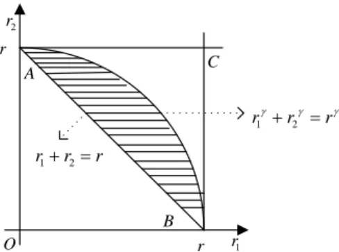
smaller than the previous. The EDS is shown in Figure4.
Energies 2016, 9, 841 5 of 17
where r is the Euclidean distance between node u and node v, is the distance-power gradient that depending on the characteristics of the communication medium (2 4, 2 for outdoor propagation modes [23]); Puv1 is the power needed for link between node u and node v.
If the transmission ranges of node u and node v are reduced based on the topology control algorithm, then node u and node v cannot communicate directly, which is shown in Figure 3. As a result, node n will be chosen as the relay node, where node n is the neighbor of both node u and node v. Thus, the energy needed to transmit packets from node u to node v will be:
2 1 2
uv
P r r, (2)
where r1 is the Euclidean distance between node u and node n, r2 is the Euclidean distance
between node n and node v; Puv2 is the power needed for communicating between node u and
node v by using relay node n.
Figure 3. Transmission range adjustment.
Therefore, the issues we need to solve are when Puv2 is smaller than Puv1 and what is the
probability that Puv2 smaller than Puv1. For exploring these issues, we define the Energy efficient
Dominating Sets (EDS) as follows:
1 2
1 2
1
2 0
0
uv uv
P P
r r r
r r
r r
, (3)
where the first constraint means the energy consumption after power adjustment is smaller than the previous one; the second constraint make sure node u still can communication with node v by using a relay node; the third and the fourth constraints guarantee the transmission ranges of each nodes are smaller than the previous. The EDS is shown in Figure 4.
1
r
2
r r
r O
A
B C
1 2
r r r
1 2
r r r
Energies2016,9, 841 6 of 17
According the definition of EDS and the principle of linear programming, the EDS is the shadow
area in Figure4. The areaABCmeans the whole values which satisfy the second, third, and fourth
constraints in Equation (3); the areaAB> is the set that the energy consumption is smaller than the
previous. Therefore, the probability that the energy consumption is less than the previous one is the
proportion of areaAB> in areaABC, which can be calculated as:
ρ= 2
r2
Z r
0 (r
γ−xγ)γ1dx−1, (4)
wherexis the transmission range of nodes and 0<x<r.
Lemma 1.With the increasing ofγ(2≤γ≤4), the probabilityρwill increase from 0.5708 to 0.8541. Proof.Considering the first derivative function ofρonγ:
ρ0γ= d[
2
r2
Rr
0(rγ−xγ) 1
γdx−1]
dγ , (5)
In order to simplify the denotation, we define:
f(γ) = (rγ−xγ)γ1, (6)
Therefore, Equation (5) can be rewritten as:
ρ0γ= d[
2
r2
Rr
0 f(γ)dx−1]
dγ , (7)
Since 0<x<r, so if we can prove f(γ)is an increasing function, then we can conclude thatρ(γ)
is also the increasing function withγ. The first derivative function of f(γ)onγis:
f0(γ) =eγ1(rγ−xγ)· γ· 1
rγ−xγ·(rγln(r)−xγlnx)−ln(rγ−xγ) γ2
>eγ1(rγ−xγ)·ln(rγ)−ln(rγ−xγ) γ2 >0
, (8)
As f0(γ) >0, so f(γ)is an increasing function. Thus, the probabilityρwill increase with the
increasing ofγ. In addition, the maximum and minimum values ofρare as follows:
ρmin=ρ2=0.5708, (9)
ρmax=ρ4=0.8541, (10)
This can also be found in Figure5.
As shown in Figure5, with the increasing ofγ, the probabilityρincreases. The maximum value of
ρis 0.8741 and the minimum value is only 0.5708. This demonstrates that the algorithm which reduces
the energy consumption by adjusting the transmission range is probabilistic, i.e., short transmission range does not mean small energy consumption. The reason why the probability increases with the
increasing ofγis that with the increasing ofγ, the energy consumption is more and more seriously
Energies2016,9, 841 7 of 17
Energies 2016, 9, 841 7 of 17
2 2.2 2.4 2.6 2.8 3 3.2 3.4 3.6 3.8 4
0.55 0.6 0.65 0.7 0.75 0.8 0.85 0.9 0.95
distance-power gradient (γ)
P
ro
ba
bi
lit
y
(ρ
)
Figure 5. The relationship between γ and ρ.
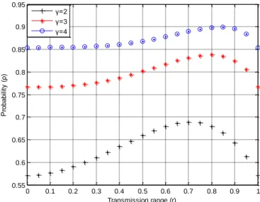
Lemma 2. With constant γ, the probability ρ will keep constant with the variation of the initial transmission range r.
Proof. We can prove this conclusion by simulation. The result can be found in Figure 6.
0 0.1 0.2 0.3 0.4 0.5 0.6 0.7 0.8 0.9 1
0.55 0.6 0.65 0.7 0.75 0.8 0.85 0.9 0.95
Transmission range (r)
P
ro
ba
bi
lit
y
(ρ
)
γ=2 γ=3 γ=4
Figure 6. Relationship between r and ρ for γ.
Figure 6 illustrates that with the increasing of r, the probability ρ will keep constant. In addition, when
γ
increases, the probability increases, too; and the bigger theγ
, the small increasing rate is, which is consistent with the conclusion of Lemma 1 (shown in Figure 5).The Lemma 2 indicates that the probability is nothing to do with the initial transmission range, i.e., no matter what r is, with constant
γ
, the probability will be the same.Lemma 3.With fixed value of
γ
, when the transmission range is(1/ 2)
1/ γr
, the probability ρe can get themaximum value.
Proof. When applying the power adjustment topology control algorithm, the EDS of
r
1 andr
2 areshown in Equation (3) and Figure 4. Thus, similar with the definition of EDS, the Un-EDS of
r
1 and2
r
can be shown as follows:1 2
1 2
1
2
0
0
uv uv
P P
r r r
r r
r r
, (11)
Figure 5.The relationship betweenγandρ.
Lemma 2.With constantγ, the probabilityρwill keep constant with the variation of the initial transmission range r.
Proof.We can prove this conclusion by simulation. The result can be found in Figure6.
Figure6illustrates that with the increasing ofr, the probabilityρwill keep constant. In addition,
whenγincreases, the probability increases, too; and the bigger theγ, the small increasing rate is, which
is consistent with the conclusion of Lemma 1 (shown in Figure5).
Energies 2016, 9, 841 7 of 17
2 2.2 2.4 2.6 2.8 3 3.2 3.4 3.6 3.8 4
0.55 0.6 0.65 0.7 0.75 0.8 0.85 0.9 0.95
distance-power gradient (γ)
P
ro
ba
bi
lit
y
(ρ
)
Figure 5. The relationship between γ and ρ.
Lemma 2. With constant γ, the probability ρ will keep constant with the variation of the initial transmission range r.
Proof. We can prove this conclusion by simulation. The result can be found in Figure 6.
0 0.1 0.2 0.3 0.4 0.5 0.6 0.7 0.8 0.9 1
0.55 0.6 0.65 0.7 0.75 0.8 0.85 0.9 0.95
Transmission range (r)
P
ro
ba
bi
lit
y
(ρ
)
γ=2 γ=3 γ=4
Figure 6. Relationship between r and ρ for γ.
Figure 6 illustrates that with the increasing of r, the probability ρ will keep constant. In addition, when
γ
increases, the probability increases, too; and the bigger theγ
, the small increasing rate is, which is consistent with the conclusion of Lemma 1 (shown in Figure 5).The Lemma 2 indicates that the probability is nothing to do with the initial transmission range, i.e., no matter what r is, with constant
γ
, the probability will be the same.Lemma 3.With fixed value of
γ
, when the transmission range is(1/ 2)
1/ γr
, the probability ρe can get themaximum value.
Proof. When applying the power adjustment topology control algorithm, the EDS of
r
1 andr
2 areshown in Equation (3) and Figure 4. Thus, similar with the definition of EDS, the Un-EDS of
r
1 and2
r
can be shown as follows:1 2
1 2
1
2
0
0
uv uv
P P
r r r
r r
r r
, (11)
Figure 6.Relationship betweenrandρforγ.
The Lemma 2 indicates that the probability is nothing to do with the initial transmission range,
i.e., no matter whatris, with constantγ, the probability will be the same.
Lemma 3. With fixed value ofγ, when the transmission range is(1/2)1/γr, the probabilityρe can get the maximum value.
Proof. When applying the power adjustment topology control algorithm, the EDS ofr1andr2are
shown in Equation (3) and Figure4. Thus, similar with the definition of EDS, the Un-EDS ofr1andr2
can be shown as follows:
Puv1≤Puv2
r1+r2≥r 0<r1≤r 0<r2≤r
Energies2016,9, 841 8 of 17
The meanings of each constraint are similar with Equation (3). The values which satisfy Un-EDS mean that the energy consumption of WSN does not decrease after reducing the transmission range. Therefore, how to reduce the size of Un-EDS is an effective method to increase the probability of energy
efficient. A possible way is to eliminate some values ofr1andr2from Un-EDS. Therefore, the new
probability of energy efficient will be:
ρe =
Rr
0(r
γ−xγ)γ1dx−r2/2
r2/2−(r−r
1)(r−r2)
, (12)
wheres= (r−r1)(r−r2)is the eliminated Un-EDS.
According the principle of linear programming, whenr1andr2are in the boundary of Un-EDS,
the eliminated Un-EDSscan get the maximum value, i.e., the probabilityρecan get the maximum
value, which can be found in Equation (12). This means thatr1andr2should satisfy the constraint
as follows:
r2= (rγ−r1γ)1/γ, (13)
The first derivative function ofsandr2onr1can be expressed as:
s0r1 =
ds dr1
=r2−r+ (r1−r)r02r1, (14)
r02r1 = dr2
dr1
=−rγ1−1(rγ−rγ1)1−γγ, (15)
Substitute Equation (15) into Equation (14), when s0r1 = 0, the eliminated Un-EDSscan get
the extremum value whenr1= (1/2)1/γr. Furthermore, when 0 <r1 < (1/2)1/γr,s0r1 >0; when
(1/2)1/γr<r1<r,s0r1 <0; sos((1/2) 1/γ
r)is the maximum value ofs. This conclusion also can be
found in Figure7. In Figure7, we set the initial transmission rangerto 1, i.e.,r=1 in this simulation.
Energies 2016, 9, 841 8 of 17
The meanings of each constraint are similar with Equation (3). The values which satisfy Un-EDS mean that the energy consumption of WSN does not decrease after reducing the transmission range. Therefore, how to reduce the size of Un-EDS is an effective method to increase the probability of energy efficient. A possible way is to eliminate some values of
r
1 andr
2 fromUn-EDS. Therefore, the new probability of energy efficient will be:
1
γ γ γ 2
0 2
1 2
( ) / 2
ρ
/ 2 ( )( )
r
e
r x dx r
r r r r r
, (12)where
s
(
r
r r
1)(
r
2)
is the eliminated Un-EDS.According the principle of linear programming, when
r
1 andr
2 are in the boundary ofUn-EDS, the eliminated Un-EDS s can get the maximum value, i.e., the probability
ρ
e can get themaximum value, which can be found in Equation (12). This means that
r
1 andr
2 should satisfythe constraint as follows:
1/γ
2
(
1)
r
r
r
, (13)The first derivative function of s and
r
2 onr
1 can be expressed as:1 1
' '
2 1 2
1
( )
r r
ds
s r r r r r
dr
, (14)
1
1 γ
' 2 1 γ
2 1 1
1
( )
r dr
r r r r
dr
, (15)
Substitute Equation (15) into Equation (14), when
1
'
0
r
s , the eliminated Un-EDS s can get the
extremum value when
r
1
(1/ 2)
1/ γr
. Furthermore, when1/ γ 1
0
r
(1/ 2)
r
,1
'
0
r
s ; when
1/ γ 1
(1/ 2)
r
r
r
,1
'
0
r
s ; so
s
((1/ 2)
1/ γr
)
is the maximum value of s. This conclusion also can be found in Figure 7. In Figure 7, we set the initial transmission range r to 1, i.e., r1 in this simulation.0 0.1 0.2 0.3 0.4 0.5 0.6 0.7 0.8 0.9 1
0.55 0.6 0.65 0.7 0.75 0.8 0.85 0.9 0.95
Transmission range (r)
P
ro
ba
bi
lit
y
(ρ
)
γ=2 γ=3 γ=4
Figure 7. Relationship between r and ρe for γ.
When the probability ρe get the maximum value, the values of
r
1 are 0.7r, 0.8r, and 0.85rwhere γ 2 , γ 3 , and γ 4 , respectively. The maximum value of ρe in Figure 7 is consistent
with the conclusion in Table 1, which are got from Equations (4) and (12). Figure 7.Relationship betweenrandρeforγ.
When the probabilityρeget the maximum value, the values ofr1are 0.7r, 0.8r, and 0.85rwhere
γ= 2,γ =3, andγ =4, respectively. The maximum value ofρe in Figure7is consistent with the
Energies2016,9, 841 9 of 17
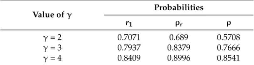
Table 1.Probabilities before and after optimizing.
Value ofγ Probabilities
r1 ρe ρ
γ= 2 0.7071 0.689 0.5708
γ= 3 0.7937 0.8379 0.7666
γ= 4 0.8409 0.8996 0.8541
From Table1, we can find that after eliminating some values from the Un-EDS, the probabilities of
energy efficient increase obviously: 11% whenγ=2, 7% whenγ=3, and 5% whenγ=4. Thus, in the
power adjustment based topology control algorithm, we can use(1/2)1/γras the optimal transmission
range of nodes.
5. Energy Efficient and Reliable Topology Control Protocol
In Section4, we proved that the optimal transmission range for getting high probability of energy
efficient is(1/2)1/γr. In this section, we propose an energy efficient and reliable topology control
protocol based on this conclusion.
In Section4, we have explored the probability of energy efficient by reducing the transmission
range in power adjustment based topology control algorithm. For guaranteeing the network
connection, in this paper, we introduce the conclusions in [24] into our algorithm as the constraints of
network reliable. In [24], the authors prove that when every node connects to its nearest 5.1774logn
neighbors, the network is asymptotic connectivity (the asymptotic connectivity means that when the
number of neighbor nodes is larger thanm, then the probability that the network is connected is
asymptotic to 1); when each node connects to less than 0.074lognnearest neighbors, the network is
asymptotic disconnectivity (the asymptotic disconnectivity means that when the number of neighbor
nodes is smaller thank, then the probability that the network is disconnected is asymptotic to 1).
The simulation result also shows that if the number of neighbors larger than 1.5logn, the probability of
connectedness increases rapidly to 1 for a modest number of nodes (e.g.,n≈30). Therefore, in ERTC,
1.5lognwill be used as the lower limitation of the neighbors number, i.e., the node degree.
There are two stages in the ERTC: (1) neighbor information collection; (2) transmission range adjustment.
5.1. Neighbor Information Collection
In this section, nodeibroadcast HELLO messagemiusing initial transmission rangerito calculate
the node degree and the distances to the neighbor nodes. As shown in Section3, the transmission range
is a circle, but may not same for each node. The HELLO messagemiincludes the transmission power
Pi, the source node IDIi, and the version numbervsiwhich is used to decide whether the received
HELLO message is a new one or not. When the neighbor nodes receive this HELLO message, firstly,
comparing the node IDIiin the HELLO messagemiwith the node IDs that in the neighbors-list; if the
node ID already exist, then check the version numbervsito find out whether this HELLO message is
a new one or not; if not, the HELLO message will be dropped immediately; otherwise, updating the
neighbor-list; in case the node IDIidoes not exist in the neighbors-list, then adding the node ID to
the neighbors-list. The distancesdijbetween two nodes are calculated when the nodeireceives the
HELLO messagemjfrom the neighbor nodes by using received signal strength indicator (RSSI) [25,26].
When the nodeireceive the HELLO messagemjfrom other nodes, they will update the neighbors-list
based on the same principle which described above and calculate the node degreeN1i.
As shown in Lemma 4, the optimal transmission range for nodeiis(1/2)1/γri, when the source
nodeireceive the HELLO messagemjfrom the neighbor nodes, it will compare the distancedijwith
(1/2)1/γri; the number of neighbor nodes whose distances to the source nodei are smaller than
Energies2016,9, 841 10 of 17
5.2. Transmission Range Adjustment
In this stage, the nodeiadjusts their transmission range according the node degree N1i and
N2i. As discussed in Section3, the optimal transmission range for energy efficient is(1/2)1/γriand
for guaranteeing the network connection, the lower limitation of the neighbors number is 1.5logn;
therefore, for meeting the requirements of both the energy efficient and the network reliability, the
node degreeN1iandN2ishould be compared with 1.5lognfor deciding the transmission range of node
i. There are three relationships between the node degree and the lower limitation of neighbor numbers
in ERTC: (1)N2i ≥1.5logn; (2)N2i ≤1.5logn≤ N1i; and (3)N1i ≤1.5logn; different relationships will
have different transmission range adjustment strategies:
(i) whenN2i ≥1.5logn, it means that when the transmission range of nodeiis(1/2)1/γri, it has the
highest probability to satisfy the requirements of both the energy efficient and network connection.
Therefore, the transmission range of nodeiis reduced to(1/2)1/γri, which is reasonable.
(ii) when N2i ≤ 1.5logn ≤ N1i, this means that when the transmission range of nodei isri, the
network connection can be satisfied; however, when the transmission range is(1/2)1/γri, it can
not meet the requirement of network connection. As shown in Figure7, when the transmission
range is close to(1/2)1/γri, the probability is close to the highest probability, too. In addition,
considering the node in ERTC is uniform distributed, so the node degreeni is proportional
with the coverage areaπr2i; therefore, the transmission range in this situation can be set to
((1.5logn)/N2i)1/2·(1/2)1/γri.
(iii) when N1i ≤ 1.5logn, this means the initial transmission range of nodei ri can not meet the
requirement of network connection. Therefore, the transmission range should be increased.
Similar with the reason in (ii), the transmission range closer to(1/2)1/γrihas higher probability
of energy efficient than that far from(1/2)1/γriand considering the node distribution in ERTC is
uniform, so the transmission range in this range can be set to((1.5logn)/N1i)1/2·ri.
The process of the ERTC is:
Energy Efficient and Reliable Topology Control Algorithm (ERTC) 1. ERTC:
Input:
2. The length of the configuration area,Border_length;
3. The number of the nodes in the network,n;
4. The value of distance-power gradient,γ;
Ensure:
5. Broadcast the HELLO messagemiwith initial transmission rangeri;
6. Receive the HELLO messagemj;
7. Update the neighbors-list;
8. Calculate the node degreeN1i;
9. Compare the distance between nodeiand the neighbor nodes with(1/2)1/γri;
10. Calculate the node degreeN2i;
11. ifN2i≥1.5lognthen
TR=(1/2)1/γri;
12. else ifN2i≤1.5logn≤ N1ithen
TR=((1.5logn)/N2i)1/2·(1/2)1/γri;
13. else
TR=((1.5logn)/N1i)1/2·ri;
14. end if
Energies2016,9, 841 11 of 17
As shown in the table above, the runtime complexity for ERTC isO(n), which is the same as the
runtime complexity of LMA and LMN [17]. Therefore, the ERTC can improve the network performance
without increasing the algorithm complexity seriously.
6. Simulation and Discussion
In this section, we will evaluate the performance of ERTC and discuss the properties in detail. ERTC is power adjustment based topology control algorithm; we compare the performance of ERTC with LMA and LMN in this paper. The reasons why the LMA and LMN are chosen as the contrasts are: (1) the ERTC is most similar to LMA and LMN and can be regarded as the extensional of
LMN and LMA based on the theory analysis in Section4; (2) LMN and LMA are the two typical and
basic power adjustment based topology control algorithms. As a contrast, we use NONE (in which there is no topology control algorithm used) as the control group.
The topology control algorithms that will be simulated in this section are as follows.
• NONE: without using topology control algorithm, i.e., forming the network topology randomly
and do not control the network topology artificially.
• LMA: in LMA, there are two node degree thresholds: the minimum threshold and maximum
threshold. If the node degree is smaller than the minimum threshold, the node will increase the
transmission range by certain factorAinc; otherwise, reducing the transmission ranges byAdec.
The nodes in which the node degrees are between the minimum threshold and the maximum threshold will not change their transmission ranges.
• LMN: in LMN, each node collects the neighbor information from their neighbors, and calculates
the average neighbors’ node degree. The value will be set as the node degree threshold. If the node degree is large than this threshold, the transmission range will be reduced; otherwise, it will be increased.
• ERTC: the algorithm proposed in this paper.
6.1. The Properties of Energy Efficient and Reliable Topology Control Algorithm
In this section, the performance and properties of ERTC will be discussed in detail. We built the simulation platform by MATLAB. The simulation parameters are presented as follows: (1) the
node number: 50–200; (2) distribution range: 1 km×1 km; (3) initial transmission range: 0–200 m;
(4) distance-power gradient: γ = 3; (5) simulation time: 3000 s; (6) initial energy supply: 100 J;
(7) transmit power: 0–1 mW; (8) receive power: 0.5 mW; (9) transmission rate: 10 kbit/s.
In Figure8, the network is formed randomly (Figure8a) and by the ERTC (Figure8b), respectively.
From Figure8, we can clearly find that the ERTC reduces the number of communication links of
the original network and guarantees the network connection at the same time. The communication
links in Figure8b are less than that in Figure8a, which means that after using the ERTC, the energy
consumption will be reduced. The node degree in Figure8b is obviously smaller than that in Figure8a;
the conclusion can be found in Figure9, too.
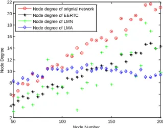
Figure9shows the node degree of the original network and the network which uses the ERTC.
From Figure9, we can conclude that with the increasing of the node number, the overall trend of
node degree is increasing. However, the node degree does not always increase with the rising of the
node number, e.g., as shown in Figure8, when the node number is 100, 105, 110, and 120, the node
degree does not keep increasing when the node number rises. The reason is that the network is created randomly, so the node degree oscillates near the average node degree; however, the overall trend is increasing. The increasing trend in ERTC is similar with the original one, but node degrees are smaller than that. In addition, when the node number is large than 100, the increasing rate of the original
network is faster than that in ERTC. Furthermore, as shown by the blue points in Figure9, with the
increasing of the node number, the increasing trends are different between the original network and
Energies2016,9, 841 12 of 17
degree in ERTC is larger than the minimum node degree threshold, so the network connection can be
guaranteed. This is consistent with the conclusion in FigureEnergies 2016, 9, 841 8b. 12 of 17
0 0.1 0.2 0.3 0.4 0.5 0.6 0.7 0.8 0.9 1
0 0.1 0.2 0.3 0.4 0.5 0.6 0.7 0.8 0.9 1 1 2 3 4 5 6 7 8 9 10 11 12 13 14 15 16 17 18 19 20 21 22 23 24 25 26 27 28 29 30 31 32 33 34 35 36 37 38 39 40 41 42 43 44 45 46 47 48 49 50 51 52 53 54 55 56 57 58 59 60 61 62 63 64 65 66 67 68 69 70 71 72 73 74 75 76 77 78 79 80 Km Km
0 0.1 0.2 0.3 0.4 0.5 0.6 0.7 0.8 0.9 1 0 0.1 0.2 0.3 0.4 0.5 0.6 0.7 0.8 0.9 1 1 1 1 2 2 2 2 2 2 2 2 2 2 2 2 2 2 3 3 3 3 3 3 4 4 4 4 5 5 5 6 6 6 6 6 6 7 7 7 7 7 7 7 7 7 7 8 8 8 8 8 8 8 9 9 9 9 9 10 10 10 10 10 10 11 11 11 11 12 12 12 12 12 12 12 12 12 12 12 12 12 13 13 13 13 13 13 14 14 14 14 14 15 15 15 15 15 15 16 16 16 16 16 16 16 16 16 16 16 16 17 17 17 17 17 17 17 17 17 17 18 18 18 18 18 18 18 18 19 19 19 19 19 19 20 20 20 20 20 20 21 21 21 21 21 21 22 22 22 22 22 22 23 23 23 23 24 24 24 24 24 24 24 24 24 24 24 25 25 25 25 25 25 26 26 26 26 27 27 27 27 28 28 28 28 29 29 29 30 30 30 30 30 30 30 31 31 31 31 31 31 32 32 32 32 32 32 32 32 32 32 32 32 32 33 33 33 33 33 33 33 34 34 34 34 34 34 34 34 35 35 35 35 35 36 36 36 36 36 36 36 36 36 37 37 37 37 37 38 38 38 38 38 39 39 39 39 39 39 39 39 40 40 40 40 40 41 41 41 42 42 42 42 43 43 43 43 43 43 44 44 44 44 44 45 45 45 45 45 45 45 45 45 46 46 46 46 46 46 46 46 46 46 46 46 46 46 47 47 47 47 47 47 47 48 48 48 48 48 48 48 48 49 49 49 49 49 49 50 50 50 50 51 51 51 51 51 51 51 52 52 52 52 52 52 52 52 52 52 52 53 53 53 53 53 54 54 54 54 54 54 55 55 55 56 56 56 56 57 57 57 57 57 57 57 57 57 58 58 58 58 58 58 58 58 59 59 59 59 59 59 59 60 60 60 60 60 61 61 61 61 61 61 62 62 62 62 62 63636363
64 64 64 65 65 65 65 65 65 65 65 65 66 66 66 66 66 67 67 67 68 68 68 68 68 68 68 68 69 69 69 69 69 69 69 69 69 70 70 70 70 71 71 71 71 71 71 71 71 71 71 72 72 72 72 72 72 73 73 73 74 74 74 74 74 74 74 75 75 75 75 75 76 76 76 76 76 77 77 77 77 77 78 78 78 78 78 78 78 78 79 79 79 79 79 80 80 80 80 80 Km Km
(a) (b)
Figure 8. The simulation result: (a) NONE; and (b) energy efficient and reliable topology control algorithm (ERTC). * The X-axis and Y-axis means the node distribution area.
50 100 150 200
2 4 6 8 10 12 14 16 18 20 22 Node Number N o d e D e g re e
Node degree of orignial network Node degree of EERTC Minimum threshold of node degree
Figure 9. The relationship between node number and node degree.
Figure 9 shows the node degree of the original network and the network which uses the ERTC. From Figure 9, we can conclude that with the increasing of the node number, the overall trend of node degree is increasing. However, the node degree does not always increase with the rising of the node number, e.g., as shown in Figure 8, when the node number is 100, 105, 110, and 120, the node degree does not keep increasing when the node number rises. The reason is that the network is created randomly, so the node degree oscillates near the average node degree; however, the overall trend is increasing. The increasing trend in ERTC is similar with the original one, but node degrees are smaller than that. In addition, when the node number is large than 100, the increasing rate of the original network is faster than that in ERTC. Furthermore, as shown by the blue points in Figure 9, with the increasing of the node number, the increasing trends are different between the original network and ERTC. The reason of this issue will be explained in the next section. Moreover, in Figure 9, the node degree in ERTC is larger than the minimum node degree threshold, so the network connection can be guaranteed. This is consistent with the conclusion in Figure 8b.
Figure 10 shows the numbers of nodes that use different transmission range adjustment strategies (introduced in Section 5) to adjust the transmission range. Since the number of nodes which use the rule (i) is pretty huge, so in Figure 10, we show the logarithm value of this number. In Figure 10, with the increasing of the node number, the nodes which use the rule (i) to adjust their transmission range has the similar increasing trend with the average node degree shown in Figure 9. Additionally, in Figure 10, the number of nodes use rule (i) is huge, and the number of nodes that use rule (ii) and rule (iii) are quite small. Since most transmission ranges will be set to (1/ 2)1/ γr
Figure 8. The simulation result: (a) NONE; and (b) energy efficient and reliable topology control
algorithm (ERTC). * TheX-axis andY-axis means the node distribution area.
Energies 2016, 9, 841 12 of 17
0 0.1 0.2 0.3 0.4 0.5 0.6 0.7 0.8 0.9 1
0 0.1 0.2 0.3 0.4 0.5 0.6 0.7 0.8 0.9 1 1 2 3 4 5 6 7 8 9 10 11 12 13 14 15 16 17 18 19 20 21 22 23 24 25 26 27 28 29 30 31 32 33 34 35 36 37 38 39 40 41 42 43 44 45 46 47 48 49 50 51 52 53 54 55 56 57 58 59 60 61 62 63 64 65 66 67 68 69 70 71 72 73 74 75 76 77 78 79 80 Km Km
0 0.1 0.2 0.3 0.4 0.5 0.6 0.7 0.8 0.9 1 0 0.1 0.2 0.3 0.4 0.5 0.6 0.7 0.8 0.9 1 1 1 1 2 2 2 2 2 2 2 2 2 2 2 2 2 2 3 3 3 3 3 3 4 4 4 4 5 5 5 6 6 6 6 6 6 7 7 7 7 7 7 7 7 7 7 8 8 8 8 8 8 8 9 9 9 9 9 10 10 10 10 10 10 11 11 11 11 12 12 12 12 12 12 12 12 12 12 12 12 12 13 13 13 13 13 13 14 14 14 14 14 15 15 15 15 15 15 16 16 16 16 16 16 16 16 16 16 16 16 17 17 17 17 17 17 17 17 17 17 18 18 18 18 18 18 18 18 19 19 19 19 19 19 20 20 20 20 20 20 21 21 21 21 21 21 22 22 22 22 22 22 23 23 23 23 24 24 24 24 24 24 24 24 24 24 24 25 25 25 25 25 25 26 26 26 26 27 27 27 27 28 28 28 28 29 29 29 30 30 30 30 30 30 30 31 31 31 31 31 31 32 32 32 32 32 32 32 32 32 32 32 32 32 33 33 33 33 33 33 33 34 34 34 34 34 34 34 34 35 35 35 35 35 36 36 36 36 36 36 36 36 36 37 37 37 37 37 38 38 38 38 38 39 39 39 39 39 39 39 39 40 40 40 40 40 41 41 41 42 42 42 42 43 43 43 43 43 43 44 44 44 44 44 45 45 45 45 45 45 45 45 45 46 46 46 46 46 46 46 46 46 46 46 46 46 46 47 47 47 47 47 47 47 48 48 48 48 48 48 48 48 49 49 49 49 49 49 50 50 50 50 51 51 51 51 51 51 51 52 52 52 52 52 52 52 52 52 52 52 53 53 53 53 53 54 54 54 54 54 54 55 55 55 56 56 56 56 57 57 57 57 57 57 57 57 57 58 58 58 58 58 58 58 58 59 59 59 59 59 59 59 60 60 60 60 60 61 61 61 61 61 61 62 62 62 62 62 63636363
64 64 64 65 65 65 65 65 65 65 65 65 66 66 66 66 66 67 67 67 68 68 68 68 68 68 68 68 69 69 69 69 69 69 69 69 69 70 70 70 70 71 71 71 71 71 71 71 71 71 71 72 72 72 72 72 72 73 73 73 74 74 74 74 74 74 74 75 75 75 75 75 76 76 76 76 76 77 77 77 77 77 78 78 78 78 78 78 78 78 79 79 79 79 79 80 80 80 80 80 Km Km
(a) (b)
Figure 8. The simulation result: (a) NONE; and (b) energy efficient and reliable topology control algorithm (ERTC). * The X-axis and Y-axis means the node distribution area.
50 100 150 200
2 4 6 8 10 12 14 16 18 20 22 Node Number N o d e D e g re e
Node degree of orignial network Node degree of EERTC Minimum threshold of node degree
Figure 9. The relationship between node number and node degree.
Figure 9 shows the node degree of the original network and the network which uses the ERTC. From Figure 9, we can conclude that with the increasing of the node number, the overall trend of node degree is increasing. However, the node degree does not always increase with the rising of the node number, e.g., as shown in Figure 8, when the node number is 100, 105, 110, and 120, the node degree does not keep increasing when the node number rises. The reason is that the network is created randomly, so the node degree oscillates near the average node degree; however, the overall trend is increasing. The increasing trend in ERTC is similar with the original one, but node degrees are smaller than that. In addition, when the node number is large than 100, the increasing rate of the original network is faster than that in ERTC. Furthermore, as shown by the blue points in Figure 9, with the increasing of the node number, the increasing trends are different between the original network and ERTC. The reason of this issue will be explained in the next section. Moreover, in Figure 9, the node degree in ERTC is larger than the minimum node degree threshold, so the network connection can be guaranteed. This is consistent with the conclusion in Figure 8b.
Figure 10 shows the numbers of nodes that use different transmission range adjustment strategies (introduced in Section 5) to adjust the transmission range. Since the number of nodes which use the rule (i) is pretty huge, so in Figure 10, we show the logarithm value of this number. In Figure 10, with the increasing of the node number, the nodes which use the rule (i) to adjust their transmission range has the similar increasing trend with the average node degree shown in Figure 9. Additionally, in Figure 10, the number of nodes use rule (i) is huge, and the number of nodes that use rule (ii) and rule (iii) are quite small. Since most transmission ranges will be set to (1/ 2)1/ γr
Figure 9.The relationship between node number and node degree.
Figure10shows the numbers of nodes that use different transmission range adjustment strategies
(introduced in Section5) to adjust the transmission range. Since the number of nodes which use the
rule (i) is pretty huge, so in Figure10, we show the logarithm value of this number. In Figure10, with
the increasing of the node number, the nodes which use the rule (i) to adjust their transmission range
has the similar increasing trend with the average node degree shown in Figure9. Additionally, in
Figure10, the number of nodes use rule (i) is huge, and the number of nodes that use rule (ii) and
rule (iii) are quite small. Since most transmission ranges will be set to(1/2)1/γr(which is the optimal
transmission range), so the network will have high probability to reduce the energy consumption. Due to the randomly formation of the network and the small number of nodes which use rule (ii)
and rule (iii), in Figure10, the statistic characteristics of these values are not regularly, so we can not
get a clear trend from these data.
The inconformity shown in Figure9(by the blue points) can be explained by the conclusion in
Figure10. In Figure10, the number of communication links that use rule (ii) when node numbers are
170, 175, and 180 are 0, 5, and 0, respectively; to the rule (iii), this numbers are 6, 0, and 0, respectively. Note that when the node number is 175, there are more nodes decrease the transmission ranges than that when the node numbers are 170 and 180; and when the node number is 170, there is more nodes
increase the transmission ranges than that when the node numbers are 175 and 180, so in Figure9, the