Real time calibration for RSS indoor
positioning systems
Ana M. Bernardos, José R. Casar, Paula Tarrío Universidad Politécnica de Madrid, Madrid, Spain {abernardos, jramon, paula}@grpss.ssr.upm.es
Abstract— Due to the random characteristics of the indoor propagation channel, received signal strength-based localization systems usually need to be manually calibrated once and again to guarantee their best performance. Calibration processes are costly in terms of time and resources, so they should be eliminated or reduced to a mínimum. In this direction, this paper presents an optimization algorithm to automatically calíbrate a propagation channel model by using a Least Mean Squares technique: RSS samples gathered in a number of reference points (with known positions) are used by a LMS algorithm to calcúlate those valúes for the channel model's constants that minimize the error computed by a hyperbolic triangulation positioning algorithm. Preliminary results on simulated and real data show that the localization error in distance is effectively reduced after a number of training samples. The LMS algorithm's simplicity and its low computational and memory costs make it adequate to be used in real systems.
Keywords — Indoor positioning, localization, calibration, optimization, LMS.
I. INTRODUCTION
The majority of indoor localization systems work with received signal strength (RSS) measurements gathered from different wireless technologies (WiFi, Bluetooth, ZigBee, etc.)- The RSS signal random nature makes these systems (using either map-based or channel model based techniques for positioning) need an off-line calibration phase - at least when starting the system for the first time.
The first objective of calibration is to characterize the noisy wireless channel, affected by multipath and fading effects. Secondly, calibration is also needed to detect (and handle) the temporal propagation dynamics originated by unstable environmental conditions (such as humidity), space reorganization (e.g. furniture re-colocation or open-closed doors) and people's movement (temporal flow, human clusters around the mobile target, etc.). For example, [1] analyzes how the average position accuracy of a fingerprint-based system (offering 2.13m. of accuracy in standard conditions - no-blocking people, close-all-doors and 40% humidity level) is deteriorated in a 43.7% when the humidity level increases until 70%, in a 236.6% if the configuration changes to all-open-doors and in a 85.9% when people clusters are present. With respect to the last issue, Chan et al. [2] shows the effects of human clustering: a group of people walking around the target user can créate strong interferences, which
make the positioning accuracy and precisión deteriórate. Finally, calibration processes are usually required when new hardware is integrated in a localization system, as the variable characteristics of transceivers chipsets, antennas and packaging of mobile devices commonly degrades the performance of the localization solution [3].
In this paper, a strategy for dynamic calibration of channel model-based localization systems is presented. We assume that the propagation channel adjust to a theoretical lognormal model, which needs to be dynamically adapted to fit the real conditions of operation. The proposed technique is based on the existence of several (position-known) reference points, on which it is possible to opportunistically take signal strength measurements (thanks to the interaction with mobile users or to a beacon-organized infrastructure). Afterwards, an algorithm iteratively calculares the valúes for the constants of the propagation channel model using real-time measurements. The adaptive algorithm works to minimize the error between the estimated position and the real one. As it is iterative - just handling data of the previous temporal instant - and simple in its formulation, the algorithm has minimum computational and memory needs; this means that it can be integrated in real-time localization systems without requiring significant resources and without introducing serious operational delays.
The remainder of the paper is organized as foliows. Section II reviews some previous proposals to automate calibration procedures for indoor localization systems. In Section III, our localization scenario is fully described. Section IV gathers the theoretic foundations of the proposed algorithm. The feasibility of the algorithm is shown in Section V through a number of experiments in a real environment. Finally, Section VI concludes the work.
II. RELATED WORK
map) of the localization área (see e.g. [4] for a review on indoor localization systems and techniques).
Calibration processes are costly and inefficient, so a line of research in indoor localization is devoted to propose solutions with zero or limited initial calibration and on-line recalibration.
For example, in the calibration phase, Gwon and Jain [5] use inter-anchor RSS measurements to genérate, for each anchor, múltiple linear functions representing the relationship between RSS and distance. During the on-line phase, a target client uses the mapping functions of the anchor with strongest RSS (Ai) to calcúlate its position to the rest of anchors (A2...An), and the mapping
function for the second anchor (A2) with strongest RSS to
calcúlate the position to Aj. A similar strategy is foliowed by Barsocchi et al. [6]; they propose a calibration strategy by which each anchor in the infrastructure broadcast a beacon that is afterwards used by other anchors to measure the reciprocal RSS. Next the localization server calibrates the propagation model parameters using these data and some information about the space's geometry, adaptively calculating the attenuation factor introduced by the walls.
Lim et al. [7] takes as input the on-line measurements of RSS between (WiFi) anchors, and between a client and its neighboring anchors, to créate a mapping between the RSS measurement and the actual geographical distance basing on the truncated singular valué decomposition technique. The algorithm does not rely on a specific propagation model, but on exploiting the fact that the RSS is inversely proportional to the distance to the power of a path loss exponent. Authors claim that the only calibration process this system requires is five minutes of measurements between pairs of anchor nodes.
Apart from stationary emitters (anchors), Krishnan et al. [8] include sniffers in their RF deployment. Sniffers are wireless transmitters that listen for all Communications from wireless clients and anchors. Authors use a spline interpolation technique on these data to build a RSS fingerprint. During the on-line localization phase, when at least one sniffer observes a significant deviation on the RSS from any emitter, the floor model is recalculated. Moraes and Nunes [9] also propose a sniífer-based technique to build a propagation map, in which each grid position is associated to a probability distribution. The map is rebuilt every T seconds or when significant variations in the RSSI occur.
In order to compénsate the environmental dynamics, Yin et al. [10] suggest temporally adapting the static RSS fingerprint. RF receivers are distributed over the space as reference points. On the signal strength valúes received both by the reference points and the mobile target, a múltiple regression analysis is used to build a corrected radio map. Information about the location of the reference points is not needed; the system works to learn the predictive relationship of signal-strength valúes between the reference points and the mobile device.
A multi-fingerprint solution to the problem of environmental dynamics is proposed by Chen et al. [1]. Information from several sensors (passive RFID,
humidity sensors, smart cards and short-range Bluetooth) serve to characterize the environmental situation in terms of humidity, open/closed doors and people and to feed an online calibration process which allows building múltiple context-aware radio maps. Following, the adaptive localization phase selects the context-aware radio map that best matches the current environmental condition state (calculated from the information coming from environmental sensors).
Zheng et al. [11] propose to automate the calibration process of an RF deployment with a time-based localization technology covering selected áreas: ultrasound trilateration is used to label RF measurements in the calibration phase. This approach may be feasible when different types of localization granularities are needed, but in most of cases will require a redundant infrastructure.
The LANDMARC system is based on deploying passive RFID reference tags to increase the accuracy of their active RFID localization strategy [12]. As described in the next Section, our general approach shares this basic idea, but applies it to the calibration problem: we propose to complete the localization infrastructure with an auxiliary structure of easily deployable and maintainable reference points, with known positions, which will serve to capture real-time RSS data which will train a propagation model by using a Least Mean Square (LMS) algorithm. As far as we know, this optimization technique has not been applied to the integration of on-line RSS measurements in propagation models, and may result in a robust and time-efficient way of performing calibration.
III. FUNDAMENTALS: LOCALIZATION SCENARIO AND
SERVICE REQUIREMENTS
Let us consider an indoor space covered by a network of anchor nodes (e.g. WiFi or Bluetooth access points, or Zigbee motes), deployed to measure the RSS of mobile targets in order to localize them. Our localization system is based on using a propagation channel model to compute each mobile-anchor node distance and perform hyperbolic triangulation.
The most popular channel model for RSS-based localization is the lognormal model [13]:
PRX(dBm) = A-10r¡\og—+N(0,a) (1)
d0
where PRX is the received power (at the receiving nodes, respectively), d is the distance between transmitter and receiver, A and r¡ are the parameters of the channel model and TV is a zero-mean Gaussian random variable with standard deviation a. A depends on the antenna gain, the transmission power and the power loss for a reference distance d0, and needs to be experimentally adjusted. The
path loss exponent r¡ has to be experimentally determined too. For example, in 2.4GHz IEEE 802.15.4 propagation, A may range between -50 and -85, while r¡ may be between 1.9 and 3.5 [15].
least to three anchor nodes. Next, the target's position is calculated by performing hyperbolic triangulation. The hyperbolic positioning algorithm may be solved with a least squares estimator (detailed formulation is available in e.g. [13]), for which the estimated coordinates (x,y) are obtained by calculating:
x
y. where
= (HTH)-1HTb
H =
2x2 2y2
2x N ¿yN_ A-RSS,
; b =
x| +
y\
-
d¡
+
d\
di = 1 0 1 0 )Í
(2)
(3)
(4)
being (x¿,y¿) the known coordinates of the i=l..N
anchors, dt the distance from the target to each anchor
with the origin of coordinates in the anchor node i=l, and RSSk the received signal strength to/from each anchor
node.
As said before, in practice, both A and r¡ need to be experimentally determined off-line and continually updated or calibrated (slightly biased estimations of A and r¡ may result in significant localization errors [13]). In this context, our objective is to avoid any off-line experimental determination of A and r¡ 1) to minimize the complexity of the calibration tasks when getting the location system to work for the first time and 2) to adapt the system's performance to real time environmental variations. To do so, we define a number of beacon or reference points located in fixed geographic locations. These reference points, easy to deploy, may be situated in waypoints (e.g. doors), attached to static objects (e.g. a printer in an office), or deployed as part of the Communications infrastructure (i.e. an anchor node could serve as reference point).
The anchor nodes will measure the RSS coming from these reference points when possible (e.g. when a user with a suitable device is detected on a reference point) and use the algorithm presented in the next section to compute A and n in real time.
Of course, this approach has many practical implementation details that are not directly addressed in this paper. For example, the number of reference points needs to be minimized, even if a technologically hybrid, low-cost and non-intrusive strategy to set them up is feasible. For example, in [12], one reference tag is needed for each square meter to provide an error distance between one and two meters; this high-density deployment is probably unrealistic in most part of common localization scenarios. Apart from that, the physical distribution of the reference points needs to be flexible, as it is not always easy to place new elements in daily-living environments. Additionally, reference points should be easily maintainable and admit dynamic reconfiguration. Assuming that a suitable deployment is feasible (as it is), the optimization algorithm used to calibrate the system is described in the next Section.
IV. THE LEAST MEAN SQUARES (LMS) ADAPTIVE
CALIBRATION ALGORITHM
Least Mean Squares is a well-known gradient-based technique to find in a computationally efficient way the valúes of the parameters of a function of data that approximates or estimates a set of reference valúes. It is based on approximating the trae gradient of the squared error of a function by its instantaneous estímate [14].
In this case, we propose to use it to set up an adaptive filter to minimize the localization error (eq. 5) by recursively adapting the constant parameters of the lognormal propagation model, A and n.
(x, y)
-RSS!
RSSj
R S S M
A(n), n(n)
i
ái
du
F(n)
Hyperbolic localization function
/' 0 \
!
(*.y)
e(ri)
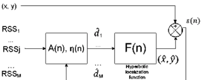
Figure 1. Adaptive filter to minimize the error in location estimation by adapting Aandt|.
Figure 1 represents how the adaptive filter works: the LMS algorithm uses the M RSS measurements taken from the calibration/reference points to iteratively calcúlate the optimal valúes of A and r¡ in each instant (iteration) n, to minimize the error between the estimated (x,y) and the (known) real position of the /' reference points (x¿,y¿). The error to be adaptively minimized is
formulated as:
5(n)-- Xi(n)-xt(n)\ +\yi{n)-yi{n)\ (5)
In Figure 1, F(n) represents the hyperbolic localization function (eqs. 1-4) which allows calculating (x,y) wúhA(n-l) and r¡(n-l); these estimated coordinates will serve to calcúlate A(n) and r¡(n) as shown in eqs. 6-7. Assuming that a single channel model is used to characterize the propagation behavior from each anchor node, the Least Mean Square algorithm is formulated as:
A, A, ,N 1 dE\£2(n)] .. ,. . sde(n)
A(n) = A(n-l)--juÁ L^ >^A{n-\)-jLiA£{n)-^>- ( f ) )
r¡{n) = r¡{n-X)-iie{n) de(n)
where //s are the filter step sizes that condition and control the speed and stability of convergence (as shown in Section V).
After detailed calculations (basically derivations and simplifications) on the formulas of hyperbolic triangulation (see [13]) the following expressions for A(n) and r¡(n) are obtained:
A(n)=A(n-l)-,,A -
i¡(n)=J¡(n-\)-^-where:
x{n) - "x{n)\ • ¿ J ¿ h « ) • loga" («) -d}(n) • logd, (n)\ +
j>W-iwl-¿D,K(»)-logi («)-¿)(«)-logí (»)]
-16-lnlO det-10-J7(H-l)
¿(n-iyuss, (8) d, =10 10'<"-1)
c, = x, •\yl+---+y2ri)-y, -{x2-y2+... + xN-yN) D, =y, \xl + ---+xlr)-x,•(x2-y2 + ---+xN-yN)
det=(i x¡+...+ 4xj,) (i y¡+... + 4 yl)-(ix2 y2+...+ 4 xNyNf
It is important to remark that the recursive valúes for A and r¡ aim at minimizing the distance error; in general, we do not seek convergence to any 'nominal' A and r¡ valúes.
V. VALIDATION AND RESULTS
The formulation above has been implemented in Matlab for validation and testing. Following, the LMS algorithm performance is shown by using both simulated and empirical data in a real scenario.
A. Simulation results
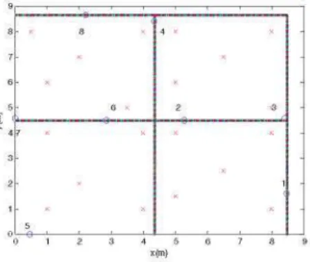
The objective of our simulation analysis has been to test the convergence of the LMS algorithm in a noisy environment. Figure 2 shows our simulation scenario, which is composed by 8 anchor nodes (serving as Communications infrastructure) and 20 reference nodes. Actually, this deployment exists in our lab and has been used for empirical validation too (see Section V.B).
Figure 2. Scenario for simulation: 4 rooms, 8 anchor nodes (o) and 20 reference (beacon) points (x).
The reference points have been randomly chosen, trying to get enough spatial diversity in each room with a modérate number of beacons (5 per room, located near the corners and the center), in order to work on a simulated but feasible scenario. In reality, these reference points should be related to objects or waypoints capable of generating 'measurement events'. For example, a door with automatic access control can serve as reference point: when a user is detected to be opening the door (e.g. by processing data from a RFID reader placed in the entonce), the localization infrastructure may trigger a 'measurement event' to request the user's mobile phone to send the (WiFi) RSS received from the nearby access points. In our simulation, 'measurement events' are generated in each reference point: 200 data arrays gathering RSS measurements from every anchor node have been simulated by using eq. 1, with PTx-Sim = 0 dBm,
d0-Sim=lm, Aim=-60 dB, nsnn=2.3 and osim=2.5 (possible
valúes for a 'standard' indoor propagation model in this geometry, as shown in [15]).
In the first iteration, the hyperbolic localization algorithm (eq. 2) has been then initialized with some given initial valúes (A0 and r¡0) and fed by a simulated
RSS array corresponding to the set of received signal strengths from a randomly chosen reference point to each anchor node. Then, we have obtained the first location estimation and its error - calculated as the mean of the error obtained in each reference point. Afterwards, the obtained valúes have served as input for eq. 6, to calcúlate the valúes for A and r¡ minimizing the distance error. Those valúes are to be used by the hyperbolic localization algorithm in the next iteration.
Figure 3. Evolution of the error (m.) in distance using a LMS filter with T|o=3, UA=0. 1, u^=0.01 and two different valúes for A: a) A>= -65
dB, b) A0= -75 dB.
Fig. 3 shows how the LMS algorithm is able to reduce the location/estimation error by adaptively adjusting A and n. The case represented in Fig. 3a. starts with a valué for A0 just differing 5 dBs from the valué used to
simúlate the RSS measurements (Asim). In this case,
approximately 100 samples are needed to calibrate the model (5 samples per reference point). When the difference between Asim and A0 is 15 dBs (Fig. 3b),
around 600 samples are needed to stabilize the error valué. In the worst case, when Asim and A0 differ in 25
dBs, approximately 4000 samples are needed (in average, 200 samples per reference point).
The limit for the distance error variance is theoretically imposed by the noise parameter a that has been used to genérate the simulated samples (also depends on r¡).
terms of needed number of RSS tupies) while providing a reasonably stable convergence valué for A and n. Although there are other valúes which may be effectively used, Figure 3 shows how the convergence works for the distance error when the filter step sizes have been set to uA=0.1, uT]=0.01. As shown in Figure 4, higher valúes of
H may accelerate the convergence (fewer samples are needed to reach the possible minimum error in distance), but may also provide a less stable convergence.
Mean error e\ol
1000 1500 2000 2500 3000 no. samples/window size
Figure 4. Effects of the valué of the LMS filter coefficients <uA, Hn>
on the mean error evolution (in m.). LMS initialization: A0= -75, T|0=3.
Simulated samples are generated with A=-60 and T|=2.3. The mean valué is calculated with a sliding window of 50 samples over the error
in distance.
Figure 5 shows how A and n evolve for several combinations of step sizes. At the beginning, all the curves have a similar behavior towards a convergence valué. Afterwards, the convergence stability is affected by the non-linear interactions between the two parameters.
— - 0 . 0 1 - 0 . 0 0 1
0.05-0.005 0.08-0.008 0.1-0.01
0.8-0.08
ípswwl
i „ J ~ J - ~ "
uo*lw-v>.:
500 1000 1500 2000
no. samples/window size
Figure 5. Effects of the valué of the LMS filter coefficients (yiA, ftq) on
the A and IJ iteratively estimated valúes. LMS initialization: An= -75 dB,
T|0=3. Simulated samples are generated with A=-60 dB and T|=2.3 dB.
The mean valué is calculated with a sliding window of 50 samples over the error in distance.
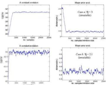
Figure 6 shows how the algorithm converges when only A is calculated with the LMS, while r¡ remains invariable. As .4 is relevant term in eq. 1, it prevails over
r¡, assuring convergence (although not to the simulation valué) even with biased (non real) valúes of r¡.
M e a n error evol.
A constant evolution
1000 1500 2000 2500 no. samples/window size
M e a n error evol.
-62
> -62.5
3 "63 -63.5
-64
( f / y i % l 4 ^
Case 4: T| = 2.1 (invariable)1000 1500 2000
no. samples
Figure 6. Evolution of A and the mean distance error when r¡ is invariable and set to a) 3 or b) 2.1. A0= -65 dB and the LMS step sizes
are uA=0.1, m=0.01. Simulated samples have been generated with A=-60 dB and T|=2.3. The mean valué is calculated with a sliding window of
50 samples over the error in distance.
B. Empirical validation
The scenario for empirical validation has the same geometry that the simulated one. It is covered by a wireless sensor network working at 2.4 GHz, composed by MicaZ motes (an IEEE 802.15.1 compliant hardware platform [16]) as anchor nodes.
With respect to the reference points, 24 beacons have been opportunistically located depending on the furniture and waypoints (doors) of the área (Fig. 7). The distribution seeks to accommodate the 'spatial diversity' and 'reasonable number of reference points' criteria used in the simulated environment, while considering the practica! feasibility of the deployment.
8
7
6
-6,
^ 4
3
2
1
•
1
5
'— ' ™ " ° ' ' > (
8
6
. • .
4
2 i
1
r
->
Figure 7. Scenario for empirical validation: 4 rooms, 8 anchor nodes (in blue color) and 24 reference points (in red color). In iteration, a
reference point is randomly selected to deliver its RSS 8-tuple.
At each reference point, a variable number of RSS measurements from each anchor node have been gathered to build a 8-tuple <RSSa, ,RSS„, (these
Propagation ohannel with A=-58 50 and eta=2 68 Mean error e\ol
Figure 8. Propagation model with real data for the 8* anchor node calculated on 24 reference points. RSS is measured in dBm, and the
propagation model parameters are A=-58.50 dB and T|=2.68.
In a real scenario, an RSS 'measurement event' may be randomly generated in any of the available beacon points (depending on the people flow and activity), or may be generated in a periodic mode (if the reference point is conceived as part of the static infrastructure). For example, a user with a wireless equipped mobile device will deliver calibration measurements when passing on a reference point (the accurate detection of the user in the reference point may be done e.g. by using RFID-NFC landmarks). Additionally, infrastructure fixed reference points (e.g. a computer with a wireless adapter) will genérate periodic tupies. So, with the obtained dataset, we have simulated the real process of calibration by feeding the LMS algorithm with tupies from randomly chosen reference points.
The performance of the algorithm is shown in Figure 9, under the same initial conditions that in the simulated scenario of the previous section, with (xA=0.1, u^O.Ol.
Mean error e\ol
500 1000 1500 2O00 25O0 3000 3500 40O0 4500 5O00 55O0 no samples/window size
Mean error e\ol
2000 3O00 4000 no. samples/wncfow size
1000 20O0 3000 4000 5000 60O0 7000 8000 9000 10000 no samples/wndow size
Figure 9. Evolution of the mean error (m) in distance using a LMS filter with T|o=3, UA=0.1, U^=0.01 and different initial valúes for A0: a)
-65 dB, b) -75 dB, c) -85. The mean valué is calculated with a sliding window of 50 samples over the error in distance.
The mean error in distance shows a decreasing trend in every case in Figure 9; this behavior may be clearly identified for low valúes of A and long-term training of the LMS algorithm. The number of samples needed to have a visible error reduction depends on the initial valué of the LMS algorithm: 1300 samples when^0= -75 dB,
and 4000 samples when^0= -85 dB (approximately 166
samples per reference points are needed). For^0= -65 dB,
the error reduction is not so observable, although after processing approximately 800 samples, the average error is below 2.2 meters.
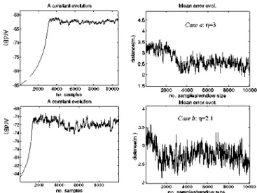
Figure 10 shows the real system's sensitivity to A (by giving r¡ a fixed valué). When.4 is variable and r¡ set to 3, the convergence valué for.4 is cióse to -65 dB. So, in the case in Figure 9, where A0= -65 dB, the error reduction is
not perceived as the best configuration for the propagation model coincides with the initial valué given toA.
Apart from that, Figure 10 shows that^ can 'converge' with very different valúes of r¡, although with different stability and error reduction. As said before, A is the dominant parameter in the lognormal propagation model (eq. 1), and it is affected by a step size one order of magnitude above the //,.
A constant evolution M e a n error evol.
>
'a. 3 -70
2000 4000 6000 8000 10000
no. samples A constant evolution
2 0 0 0 4 0 0 0 6 0 0 0 8 0 0 0 1 0 0 0 0 no. samples/window size
M e a n error evol.
2000 4000 6000 8000
no. samples
Figure 10. a) Evolution ofA and mean distance error when //is invariable and set to a) 3, b) 2.1; A0= -85 dB. The LMS step sizes are
VI. CONCLUSIONS AND FURTHER WORK REFERENCES
Preliminary results in Section V and VI show that our LMS strategy for calibration is feasible and promising. The algorithm is capable to adapt the parameters of a lognormal propagation model to provide minimized errors in distance when using a hyperbolic localization technique.
The proposed algorithm is simple and lightweight in terms of computational needs and memory requirements: it performs iteratively on real-time data and the estimation obtained in the previous instant. For this reason, we find it especially attractive to assist localization systems in their calibration tasks, and also to embedded it in resource-constrained hardware (such as MicaZ motes) to perform distributed calibration.
In order to enhance the algorithm accuracy, we are currently testing the effect of handling various propagation models (one per anchor node, one per anchor node and room) and additional information about the physical structure of the environment (e.g. walls) to demónstrate if additional complexity in channel modeling may benefit the algorithm performance. Another idea we are working on is about sequencing the estimation of A and n, instead of doing joint computation. In the same line, we are also considering its integration with other localization algorithms (circular and weighted hyperbolic and circular).
From a practical viewpoint, an in-depth analysis about the relationship between the number of reference points, their geometrical distribution and the LMS algorithm accuracy is needed. It is also necessary to study the processing time the algorithm needs, in order to adjust the LMS step sizes to effectively work in real environments.
Together with the algorithm enhancement, it is necessary to explore how to easily deploy technologically-hybrid, unobtrasive and reconfigurable reference points in real environments, which guarantee the interaction with potential users to acquire sufficient calibration data in real-time operation.
As the reader will notice, there is still a way to go to have a fully operative solution. In summary, further work is focused on demonstrating the stability of the proposal in real time operation, to show that the system can effectively adapt its behavior to real dynamic changes in the localization environment.
ACKNOWLEDGMENTS
This work has been supported by the Government of Madrid under grant S-2009/TIC-1485 and by the Spanish Ministry of Science and Innovation under grant TIN2008-06742-C02-01. Authors acknowledge Henar Martín and Inés Ortega for their help with the empirical work.
[I] Y. C. Chen, J. R. Chiang, H. H. Chu, P. Huang, A. W. Tsui, "Sensor-assisted WiFi Indoor Location System for Adapting to Environmental Dynamics", Proc. ofMSWiM, 2005.
[2] L. Chan, J. Chiang, Y. Chen, C. Ke, J. Hsu, H. Chu. Estimation with Neighborhood Links in Clusters", Proc. ofthe International
Conference onPervasive Computing, pp. 50-66, 2006.
[3] A. W. Tsui, Y-H. Chuang, H-H. Chu, "Unsupervised Learning for Solving RSS Hardware Variance Problem in WiFi Localization",
MobileNetw. Appl., 14:667-691, 2009.
[4] H. LUÍ, H. Darabi, P. Banerjee, J. Liu, "Survey of Wireless Indoor Positioning Techniques and Systems", IEEE Trans. on Systems,
Man and Cybernetics — Parí C: Applications and Reviews, vol. 37,
no. 6, November 2007.
[5] Y. Gwon, R. Jain, "Error Characteristics and Calibration-free Techniques for Wireless LAN-based Location Estimation". Procs.
Of the Second International Workshop on Mobility Management & Wireless Access Protocols (pp. 2-9), ACM, 2004.
[6] P. Barsocchi, S. Lenzi, S. Chessa, G. Giunta, "A Novel Approach to Indoor RSSI Localization by Automatic Calibration of the Wireless Propagation Model", Procs. of the 69"1 Conf on
Vehicular Technology Conference, pp. 1-5, 2009.
[7] H. Lim, L-C. Kung, J.C. Hou, H. Luo. "Zero-configuration, robust indoor localization: Theory and Experimentation", Proc. IEEE
INFOCOM 2006 25TH IEEE International Conference on Computer Communications, pp. 1-12, IEEE Computer Society,
2006.
[8] P. Krishnan, A.S. Krishnakumar, W-H. Ju, C. Mallows, S. Ganu, "A system for LÉASE: Location Estimation Assisted by Stationary Emitters for Indoor RF Wireless Networks", Procs. of
INFOCOM, pp. 1001 - 1011, vol.2, 2004
[9] L.F.M. de Moraes, B.A.A. Nunes, "Calibration-Free WLAN Location System Based on Dynamic Mapping of Signal Strength",
Procs. of the 4th ACM international workshop on Mobility management andwireless access, pp. 92 - 99, 2006.
[10] J. Yin, Q. Yang, L. Ni, "Adaptive Temporal Radio Maps for
Indoor Location Estimation", Procs. ofthe 3rd IEEE Int. Conf. on Pervasive Computing and Communications, 2005.
[II] V. W. Zheng, J. Zhao, Y. Wang, Q. Yang, "HIPS: A Calibration-less Hybrid Indoor Positioning System Using Heterogeneous
Sensors", Procs. of the IEEE Int. Conf. on Pervasive Computing and Communications, 2009.
[12] L. M. Ni, Y. Liu, Y. C. Lau, A. P. Patil, "LANMARC: Indoor Location Sensing using Active RFID," Wireless Networks, vol. 10, no. 6, pp. 701-710, Nov. 2004.
[13] P. Tarrío, A.M. Bernardos, J.R. Casar. "An RSS Localization Method based on Parametric Channel Models", Proceedings ofthe
International Conference on Sensor Technologies and Applications, pp. 265-270, IEEE Computer Society, 2007.
[14] B. Widrow, J.M. McCool, M.G. Larimore, C.R. Jr. Johnson. "Stationary and nonstationary learning characteristics ofthe LMS adaptive filter,"Proc. IEEE: vol. 64:pp. 1151-1162, Aug. 1976. [15] P. Tarrío, H. Martín, A.M. Bernardos, "Enhancing the
Performance of Propagation Model-Based Positioning
Algorithms", Procs. ofthe 3' International Workshop on User-Centric Technologies and Applications, pp. 123-132, 2009.