Variability of extreme precipitation over Europe and its relationships with teleconnection patterns

(1)

Hydrol. Earth Syst. Sci., 18, 709–725, 2014 www.hydrol-earth-syst-sci.net/18/709/2014/ doi:10.5194/hess-18-709-2014

Hydrology and

Earth System

Sciences

Open Access

Variability of extreme precipitation over Europe and its

relationships with teleconnection patterns

A. Casanueva1, C. Rodríguez-Puebla2, M. D. Frías1, and N. González-Reviriego2

1_{Grupo de Meteorología, Dpto. Matemática Aplicada y Ciencias de la Computación, Univ. de Cantabria,}

Avda. de los Castros, s/n, 39005 Santander, Spain

2_{Dept. of Atmospheric Physics, Plaza de la Merced S/N, University of Salamanca, Salamanca, Spain}

Correspondence to: A. Casanueva (ana.casanueva@unican.es)

Received: 4 September 2013 – Published in Hydrol. Earth Syst. Sci. Discuss.: 15 October 2013 Revised: 13 January 2014 – Accepted: 14 January 2014 – Published: 19 February 2014

Abstract. A growing interest in extreme precipitation has

spread through the scientific community due to the effects of global climate change on the hydrological cycle, and their threat to natural systems’ higher than average climatic val-ues. Understanding the variability of precipitation indices and their association to atmospheric processes could help to project the frequency and severity of extremes. This paper evaluates the trend of three precipitation extremes: the num-ber of consecutive dry/wet days (CDD/CWD) and the quo-tient of the precipitation in days where daily precipitation exceeds the 95th percentile of the reference period and the to-tal amount of precipitation (or contribution of very wet days, R95pTOT). The aim of this study is twofold. First, extreme indicators are compared against accumulated precipitation (RR) over Europe in terms of trends using non-parametric approaches. Second, we analyse the geographically opposite trends found over different parts of Europe by considering their relationships with large-scale processes, using differ-ent teleconnection patterns. The study is accomplished for the four seasons using the gridded E-OBS data set developed within the EU ENSEMBLES project.

Different patterns of variability were found for CWD and CDD in winter and summer, with north–south and east–west configurations, respectively. We consider physical factors in order to understand the extremes’ variability by linking large-scale processes and precipitation extremes. Opposite asso-ciations with the North Atlantic Oscillation in winter and summer, and the relationships with the Scandinavian and East Atlantic patterns as well as El Niño/Southern Oscilla-tion events in spring and autumn gave insight into the trend differences. Significant relationships were found between the

Atlantic Multidecadal Oscillation and R95pTOT during the whole year. The largest extreme anomalies were analysed by composite maps using atmospheric variables and sea sur-face temperature. The association of extreme precipitation indices and large-scale variables found in this work could pave the way for new possibilities regarding the projection of extremes in downscaling techniques.

1 Introduction

The occurrence of extreme events and their impacts on so-ciety have become a fundamental issue due to the greater climate change effects on them than on mean values caus-ing, for example, damages related to health, agriculture, en-ergy and tourism. Broad knowledge about extremes would allow for a better adaptation to new climatic conditions and reduce the damage of climate change (IPCC, 2012). Heat- and cold waves, very heavy precipitation episodes, and droughts are examples of climate extremes related to the tails of frequency distributions. Other definitions of cli-mate extremes refer to the occurrence of a variable above (or below) a threshold. The predictions announced by the IPCC (Intergovernmental Panel on Climate Change) reports (IPCC, 2012) indicate that extreme events are very likely to change in intensity, frequency and location in 21st century (see e.g. Easterling et al., 2000; Tebaldi et al., 2006). This IPCC report points out human influence as a likely cause of global warming and changes in the hydrological cycle, with a precipitation decrease in subtropical areas and intensifica-tion of extremes (Trenberth, 2011). The interest surrounding

(2)

monitoring extreme events is addressed in Donat et al. (2013) and Peterson et al. (2013), who compared results of the in-dices for different gridded data sets for the entire globe and for the US. At a regional scale, the Mediterranean and north-eastern European regions have been identified as primary climate-change hot spots (Giorgi, 2006), which motivates the study of extremes on this continent. Since climate extremes have occurred throughout history (Schonwiese et al., 2003; Tank and Konnen, 2003), individual extremes can not be sim-ply and directly attributed to anthropogenic climate change, because they can be included in the limits of the broad natural variability. However, the changes in the frequency of climate extremes may be related to global warming due to variations and shifts of atmospheric circulation. van den Besselaar et al. (2012) show different trend patterns over Europe depending on the season, highlighting the need to link precipitation ex-tremes to atmospheric flow patterns.

Although extreme indicators have been widely used to analyse extreme events in different regions over Europe (see e.g. Schonwiese et al., 2003; Kostopoulou and Jones, 2005; Hidalgo-Muñoz et al., 2011), here we present the study for the entire continent and try to relate the opposite trends in different regions with teleconnection patterns; therefore, we examine the impact of large-scale variables on extremes to have some criteria for the statistical downscaling of extremes under a warming climate. Moreover, we compare mean pre-cipitation to extreme prepre-cipitation indices.

Teleconnections refer to associations of climate system anomalies, both atmospheric and oceanic, that take place over long distances (Barnston and Livezey, 1987). They gov-ern the variability of the climate system in different spa-tial and temporal scales, being one important issue for the atmospheric science. Several Northern Hemisphere telecon-nection patterns are considered in this study in order to find associations with the precipitation extremes over Europe: the North Atlantic Oscillation (NAO), the Scandinavian Pattern (SCAND), the East Atlantic Pattern (EA) and the East At-lantic/Western Russia Pattern (EAWRUS). Also the Southern Oscillation Index (SOI), the Atlantic Multidecadal Oscilla-tion (AMO) and the Madden–Julian OscillaOscilla-tion (MJO) were taken into account due to their interannual and decadal os-cillations. These teleconnection patterns have been related in the literature to common atmospheric variables such as tem-perature and precipitation, but also to river flows, snow cover, or cereal production (see e.g. Rodríguez-Puebla et al., 2007; Carril et al., 2008; Vicente-Serrano et al., 2009; Brands et al., 2013).

The aim of this study is twofold, on the one hand we describe the main features of the precipitation extremes in Europe using indicators derived seasonally from the E-OBS data set (Haylock et al., 2008). On the other hand, we con-sider some processes of the atmospheric circulation by link-ing teleconnection patterns with precipitation indices in order to explain the non-stationarity of extremes. Firstly, a statis-tical descriptive study and a trend analysis of precipitation

extreme indicators are calculated over all of Europe. Sec-ondly, we try to interpret the opposite trend patterns found over different European regions by considering their relation-ships to the main modes of circulation variability.

The manuscript is structured as follows. In Sect. 2 we de-scribe the data and in Sect. 3 the methodology applied. Main results are presented in Sect. 4 for each season. Compari-son of different results and main conclusions are presented in Sect. 5.

2 Data

2.1 Precipitation data

Daily precipitation data from the E-OBS data set (ver-sion 5.0) were used with a resolution of 0.5◦_{, for the} pe-riod from 1950 to 2010 (Haylock et al., 2008; Hofstra et al., 2009). This data set has been developed within the framework of the EU ENSEMBLES Project (http://www. ensembles-eu.org) and represents the first freely available daily data with very high resolution covering Europe. This data set has been obtained by interpolation of observed data from more than 2300 stations over Europe. It presents ad-vantages with respect to previous products because of the higher spatial resolution, the time and spatial coverage and the larger number of stations used. Particularly, this version increases the number of stations in Spain and Germany.

2.2 Teleconnection patterns

In this study, the variability of extremes over Europe is re-lated to different Northern Hemisphere teleconnection pat-terns: the Arctic Oscillation (AO), the North Atlantic Oscil-lation (NAO), the Scandinavian Pattern (SCAND), the East Atlantic Pattern (EA) and the East Atlantic/Western Russia (EAWRUS). Also the Southern Oscillation Index (SOI) from the Tropical Pacific, the Atlantic Multidecadal Oscillation (AMO) and the Madden–Julian Oscillation (MJO) have been found to affect precipitation. The behaviour of these telecon-nection patterns changes during the year. For instance, the summer NAO differs significantly from the winter and spring pattern, and also the leading Empirical Orthogonal Function (EOF) mode of the summer precipitation has a spatiotem-poral structure which is principally different from those of the winter and spring seasons (Zveryaev, 2006). According to this, it seems appropriate to analyse the relationships be-tween teleconnections and precipitation seasonally.

It is widely known that the NAO modulates precipitation in Europe (see e.g. Trigo et al., 2004; Zorita et al., 1992), and particularly, it justifies most of the interannual variability of winter precipitation over Spain (Rodríguez-Puebla et al., 2001) and also affects the intensity and frequency of extreme precipitation in different regions over the Iberian Peninsula (Vicente-Serrano et al., 2009). The NAO mostly explains the precipitation variability in Europe, nevertheless there are

(3)

A. Casanueva et al.: Extreme precipitation and teleconnections in Europe 711

other modes of variability such as the EAWRUS, the SCAND or the EA (Ramos et al., 2010) which are also related. For in-stance, Bueh and Nakamura (2007) found that the positive SCAND phase causes a decrease in fall precipitation over northeastern Europe. The EA pattern is widely described in Wallace and Gutzler (1981), and Rodríguez-Puebla et al. (2001) show the important role of the EA and EAWRUS to explain the precipitation variations in the northern part of the Iberian Peninsula in winter. We also include one global in-dex on the tropical Pacific, the SOI. This atmospheric inin-dex is related to the El Niño pattern, which consists of the first mode of variability of the global sea surface temperature. It is responsible for the precipitation regime not only in the central and eastern Pacific, it is also related to droughts in Brazil and Australia, the Indian monsoon and the flow of the Nile River (see e.g. Ropelewski and Halpert, 1987; Hoerling and Kumar, 2000). Moreover, Rodo et al. (1997) and Frias et al. (2010) have related this index to the precipitation on the Iberian Peninsula in spring and autumn. We also considered an oceanic teleconnection pattern, the AMO (Enfield et al., 2001; Dima and Lohmann, 2007). Apart from its relation to precipitation in North America, the AMO warm phase rein-forces the Indian and Sahel monsoons and the cyclonic activ-ity in the north of the Atlantic (Zhang and Delworth, 2006).

Some studies indicate the influence of the tropical con-vection modes on the large-scale perturbations (Vitart and Molteni, 2010) and on precipitation patterns (Higgins et al., 2000; Zhou et al., 2012) or river flows (Massei and Fournier, 2012). The propagation of tropical convection can be rep-resented by the Madden–Julian Oscillation (MJO) (Madden and Julian, 1994; Zhang, 2005; Wheeler and Hendon, 2004; Gottschalck et al., 2010). The MJO index is based on a combined Empirical Orthogonal Function (EOF) analysis us-ing fields of near-equatorially averaged 850 hPa and 200 hPa zonal wind and outgoing longwave radiation (OLR). This is the dominant mode of intraseasonal variability across the global tropics and is a fluctuation of tropical circulation with a period between 30 and 60 days. According to Vitart and Molteni (2010), the MJO is a major source of predictability in the extratropics in the sub-seasonal timescale. It plays an active role in the onset and development of an El Niño event and also impacts the extratropical weather. Cassou (2008) claims that the MJO controls part of the distribution and sequences of the four daily weather regimes defined over the North Atlantic–European region in winter (i.e. NAO+, NAO−, Atlantic ridge and Scandinavian blocking), being the most affected NAO regimes. The probability of a positive phase of the NAO is significantly increased (decreased) fol-lowing an MJO in phase 3 (phase 6). Roundy et al. (2010) demonstrate that the MJO influence on the NAO is greater during La Niña conditions and when both modes (ENSO and MJO) are present at the same time, both need to be considered simultaneously to diagnose the associated global weather patterns. Although the linear response to ENSO over Europe is small, it might influence the weather over Europe

by amplifying and modulating the sign of the extratropical response to the MJO over the North Atlantic.

The time series of these indices were obtained from the Climate Prediction Center (CPC) and the NCEP NOAA web site (http://www.cpc.noaa.gov/data/) for the same period as the E-OBS data (MJO for 1979–2012 only).

To attribute the causes of the largest or most significant precipitation extremes we have also considered the sea level pressure and wind at the surface, and velocity potential at 200 hPa level from the NCEP/NCAR reanalysis data (Kalnay et al., 1996), since teleconnection patterns affect the atmo-spheric conditions at different levels. The velocity potential is computed from horizontal winds at 200 hPa and as shown below, it identifies regions where there is convergent (diver-gent) winds and consequently subsidence (rising air) and less (high) precipitation. We also use the extended reconstructed sea surface temperature (ERRST v3b) (SST) (Smith et al., 2008) from the National Climatic Data Center of the Na-tional Oceanic and Atmospheric Administration (NOAA) of the US.

3 Methodology 3.1 Extreme indicators

Within the framework of the World Meteorological Or-ganization, the Expert Team on Climate Change Detec-tion and Indices (ETCCDI, http://etccdi.pacificclimate.org/ indices_def.shtml), deals with the definition of climate ex-tremes in order to obtain comparable results in different countries. Here we address the study of some precipitation extreme indices derived from precipitation for the four sea-sons: winter (DJF), spring (MAM), summer (JJA) and au-tumn (SON) due to different influences through the year. Ta-ble 1 shows the indicators considered in this study.

Although there are other precipitation extreme indices, here these three indicators were chosen because they are use-ful to represent both dry (CDD) and wet (CWD, R95pTOT) conditions. As CDD and CWD are related to the precipi-tation occurrence, they can characterize droughts indirectly which are of great interest, for instance, for agricultural ac-tivities. Moreover, R95pTOT determines the intensity of very heavy events, examining the contribution of the 5 % more extreme days to the total precipitation, which in the case of Spain clearly separates the different extreme regimes of the Atlantic and Mediterranean climates. This index quantifies very extreme events, which can be responsible for floods and soil erosion. In addition, these three indicators are related to different driving mechanisms. As presented in the following sections, CWD and CDD are more related to large-scale at-mospheric circulation, while R95pTOT has a convective ori-gin and depends more on local processes and moisture fluxes.

(4)

Table 1. Extreme indicators considered in the study.

Acronym Definition Unit

CWD Consecutive wet days days

CDD Consecutive dry days days

R95pTOT Quotient of the precipitation in days where daily precipitation exceeds the 95th percentile of the reference period %

and the total amount of precipitation

3.2 Trend analysis

The E-OBS data were first analysed by means of a basic sta-tistical description in order to explore the data distribution. The results of the statistical properties allow us to infer re-gions more sensitive to suffering from changes in climate stationarity. Then, a trend analysis was performed using the Mann–Kendall test (Kendall, 1975) together with the Sen’s test (Sen, 1968). The former allows us to investigate long-term trends of data without assuming any particular distribu-tion and it is less influenced by outliers as it is a nonparamet-ric test. The latter is based on the Kendall’s rank correlation tau and it is calculated as the median of the set of slopes joining pairs of points. On the one hand, the Sen’s slope es-timates the magnitude of the variable–time relationship by means of a nonlinear procedure, and on the other hand, the Mann–Kendall test (Z Kendall’s coefficient) gives us the sig-nificance of the trend.

The resulting dipolar structures of the trend patterns are expected to reflect the different influence of atmospheric cir-culation. Therefore, we consider the relationships between precipitation (mean and extreme) and the teleconnection pat-terns to give insight into the physical causes for that long-term variation.

3.3 Relationship with teleconnection indices

The Empirical Orthogonal Functions (EOFs) method is ap-plied to identify spatial and temporal variability (Jolliffe, 2002; Wilks, 2006). Lorenz (1956) was the first to apply this mathematical artefact to meteorological studies. The EOFs are parameters of the covariance matrix of data anomalies. Different procedures can be used to calculate the eigenvec-tors and eigenvalues (von Storch and Zwiers, 1999). In this study, we apply the Principal Component Analysis (PCA) to time series of extreme indicators (and also mean precipita-tion) in order to characterize extremes by regions. As a result, the first EOFs are the spatial patterns corresponding to the places with the highest variability and the associated scores or Principal Components (from now on denoted as PCs) are the time series related to these places (i.e. PC1 corresponds to EOF1 and so on). This analysis also provides the variance or eigenvalue associated with each PC. We focus the study on the first and second modes of variability, since they are sep-arated (in terms of explained variance) (North et al., 1982)

and can be physically interpreted when they are compared to the teleconnection patterns as shown below.

This part of the study remarks on the relevance of analysing the influence of teleconnection patterns on precip-itation extremes to find the explanations for their variabil-ity and, hence, to justify the different trend patterns found in the extremes. Due to the limitations of global climate model outputs for hydrological applications, this work could pave the way for new possibilities for the projection of extremes. Projections of the changes in precipitation extremes are as-sociated with local variations, mainly due to the increase of water vapour as the warming increases. However, the projec-tions of extreme precipitation for larger areas can be related to the fluctuations of large-scale modes of variability.

4 Results

The spatial distribution of the extreme indicators (Fig. 1) is first analysed using the E-OBS data set for every season (by columns) and for the period of study (1950–2010). The high-est values of CDD (first row) are found in the Mediterranean Basin, especially the Iberian Peninsula and the Balkans, in every season. The places with the highest number of CWD (second row) are similar to those with more RR, included as Fig. S1 in the Supplement. The maps for R95pTOT (third row) present the highest values in the south of the continent, especially in the southwestern Iberian Peninsula in summer and in the whole Mediterranean Basin in the other seasons. The standard deviation is always higher in places with more (mean or extreme) precipitation.

The comparison of the trend tests for the seasonal mean precipitation (RR) and the three extreme indicators (CDD, CWD and R95pTOT) and the regionalization by using the EOF analysis are shown in the following sections for each season: winter, spring, summer and autumn.

4.1 Winter

Figure 2 shows the results from the Z and Sen trend tests for RR, CDD, CWD and R95pTOT in winter. The shadings rep-resent the Sen’s slope per decade (bluish (brownish) colours mean wetter (drier) conditions), in order to express decadal changes. The black dots correspond to those points where the trends are statistically significant at 5 % significance level ac-cording to Z Kendall’s coefficient.

(5)

Fig. 1. Seasonal mean distribution of CDD (days), CWD (days) and R95pTOT (%) for the different seasons (columns).

Winter precipitation tends to decrease in some areas in the south but increases significantly in the north, which is in agreement with van den Besselaar et al. (2012). However, very extreme precipitation (R95pTOT) tends to increase in sparse areas in the north, centre and south of the continent. The number of CWD tends to decrease, especially in the Iberian Peninsula, and increase in the northeast of the con-tinent, while the increase of the number of CDD extends to the whole Mediterranean Basin. More significant trends were found for extremes than those for mean precipitation.

Due to the dipolar structures found in CDD, CWD and RR trends, the analysis of extremes here is related to telecon-nection patterns to connect extremes variability to modes of low-frequency variability. These relationships are first anal-ysed in terms of correlation between the teleconnection in-dices and the leading Principal Components (PCs) of the ex-treme indices. Results derived from this approach allow us to choose the teleconnection patterns that mainly influence the extreme precipitation over Europe. The correlation val-ues obtained for winter are presented in Table 2. These valval-ues

are calculated for the data without trend to avoid the overesti-mation of the correlation coefficients due to the trend effect. Values in brackets show the variance of each PC (in %).

In winter, the first PC for both mean and extreme pre-cipitation (CDD and CWD) shows the highest correlation with the NAO. Some other significant correlations have been found between the EA, EAWRUS and SCAND patterns and upper-order PCs. Another interesting outcome is that we found the highest relation for the very extreme precipita-tion (R95pTOT) with the Atlantic Multidecadal Oscillaprecipita-tion (AMO). Since this kind of extreme event must depend more on convective precipitation than on large-scale precipitation, it is reasonable to be modulated by this oceanic index, rather than the usual winter circulation regimes. Notice that espe-cially for winter, the explained variance by the PC1 for RR is higher than that for the extremes, since it varies with greater spatial coherence. Haylock and Goodess (2004) previously noted that the variance for the extreme indicators compared with mean values is lower because of the noisier nature of extremes and the large size of the region under study.

(6)

Fig. 2. Trend maps of RR, R95pTOT, CDD and CWD in winter. Shadings represent the Sen’s slope per decade (bluish (brownish) colours

mean wetter (drier) conditions). The black dots correspond to those points where the trends are statistically significant at 5 % significance level (Z Kendall’s coefficient).

Table 2. Correlation coefficients between the leading PCs of mean and extreme precipitation and the teleconnection indices in winter. The

variance of each principal component is shown in brackets. Only significant values are shown (∗∗pvalue < 0.01,∗pvalue < 0.05).

NAO EA EAWRUS SCAND AMO

RR-PC1 (39 %) −0.68 ± 0.06∗∗ 0.34 ± 0.11∗∗ −0.48 ± 0.09∗∗ 0.51 ± 0.09∗∗ – RR-PC2 (16 %) 0.32 ± 0.12∗ 0.52 ± 0.09∗∗ −0.29 ± 0.11∗ – – CDD-PC1 (26 %) 0.56 ± 0.11∗∗ – 0.56 ± 0.07∗∗ −0.47 ± 0.09∗ – CDD-PC3 (8 %) – −0.47 ± 0.09∗∗ – – – CWD-PC1 (22 %) −0.73 ± 0.06∗∗ – −0.45 ± 0.09∗∗ 0.54 ± 0.09∗ – CWD-PC2 (13 %) – 0.55 ± 0.09∗∗ −0.45 ± 0.10∗∗ – – R95pTOT-PC1 (17 %) – – – – 0.54 ± 0.09∗∗ R95pTOT-PC3 (4 %) 0.41 ± 0.10∗∗ – – −0.33 ± 0.13∗∗ –

Correlation maps for the most significant relationships found in Table 2 are analysed in more detail. Figure 3 (shad-ings) shows the correlation values (× 100) between the NAO, the EAWRUS and the EA (in rows) with winter RR, CDD and CWD (in columns). Only significant values at 5 % sig-nificance level are shown. Contour lines represent the EOF associated with the PC with significant correlation in Table 2 (e.g. the upper-left map shows the spatial correlation between the RR and the NAO in shading, and contour lines repre-sent the first EOF (EOF1) from the RR, while the lower-left

map shows the spatial correlation between the EA and the RR in shading, and the contour lines represent the second EOF (EOF2) from the RR). Note that positive EOF patterns are plotted with solid lines and negative EOF with dashed lines. A north–south dipole of correlation values with the NAO is observed over Europe. The same dipole is shown by the main pattern (EOF1) representing the variability of RR, CWD and CDD. The NAO is negatively correlated to the RR and CWD in the south of the continent and positively in the north, while the EOF1 from RR and CWD are negative in the north and

(7)

Fig. 3. Shaded regions represent the correlation coefficients (× 100) between the teleconnection indices (NAO, EAWRUS, EA by rows) and

the mean or extreme precipitation fields (by columns) in winter. Contour lines represent the EOF associated with the PC better correlated with the teleconnection index according to Table 2.

positive in the south. The opposite behaviour is found for CDD (Fig. 3, first row, third column). Therefore, positive phases of the NAO cause heavier precipitation and an in-crease in CWD (dein-crease in CDD) in the north of Europe and the opposite in the south of the continent. The contrary would happen for negative phases. The correlation of these variables with the EAWRUS is shown in Fig. 3 (second row). Also in this case the EOF1 (contour lines) fits the significant corre-lated areas (shaded regions). The correlation with this pattern is negative (positive) for RR and CWD (CDD) in the south and the British Isles, whereas the opposite is found over Nor-way. The positive EOF2 of RR (contour lines in Fig. 3, third row, first column) discriminate the Atlantic Basin of the con-tinent and that fits with the region where the RR and EA are more related, in particular, positively associated. Then, pos-itive phases of the EA lead to more precipitation (mean and

extreme) in those areas. R95pTOT presents a positive corre-lation with the AMO; positive phases of AMO would then increase very extreme precipitation in sparse regions of the continent. The EOF1 of this extreme index does not show any regionalization, so this figure is not shown for any season.

The north–south dipole found for the correlation with the NAO and EAWRUS agrees with the spatial structure found in the trend analysis, meaning that teleconnections could be influencing the trend of CDD, CWD and RR besides other interannual variability. To support this idea, we exam-ine the atmospheric processes contributing to the variabil-ity of CDD and CWD by grouping the years when their principal components have greater (lower) values than the mean plus (minus) the standard deviation (SD) multiplied by 1.5. Thus we consider approximately 10 % of data as most anomalous extremes. For those years the composite

(8)

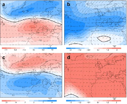
Fig. 4. Composite maps of SLP (hPa) and wind (m s−1) at 850 hPa (a) and velocity potential (× 106m2s−1) at 200 hPa (b) for extreme CWD (PC1) in winter. Same maps for the NAO (c and d).

maps of sea level pressure (SLP) and velocity potential at 200 hPa are shown in Fig. 4 for the case of CWD (first row), since this extreme shows greater decreasing trend in a large area over south-central Europe. We found a dipolar struc-ture with negative SLP anomalies over southwestern Europe and positive anomalies over subpolar areas (Fig. 4a). At up-per levels (Fig. 4b) we obtain negative values for velocity potential, which means divergent winds over Europe. These atmospheric properties are occurring during NAO negative phases, in agreement with results depicted on Table 2. Fig-ure 4c, d shows the composite maps of SLP and velocity po-tential corresponding to the years with the largest anomalies of the NAO i.e. when the index exceeds the mean ±1.5 SD. There is correspondence between the positive and negative anomalies of Fig. 4a, c. At upper levels there is also agree-ment between Fig. 4b, d with negative and positive veloc-ity potential, respectively. These figures confirm the opposite relationships between NAO and CWD, providing sources of CWD predictability that arises from the links between ex-tremes and low and upper level atmospheric variables.

To illustrate the effects of MJO on precipitation over Eu-rope we obtained composite maps for precipitation (RR), sea level pressure (SLP) and sea surface temperature (SST) dif-ferences for the years when phase 3 of the MJO exceeds the mean value ±SD (as Vitart and Molteni, 2010). We used phase 3 of the MJO (centred in 120E) because it represents an area of enhanced convection over the eastern Indian Ocean,

where the largest MJO anomalies are found, and because of its association to ENSO patterns with inter-annual fluctua-tions (Hoell et al., 2013). Moreover, as mentioned before, Cassou (2008) showed that the impact of the MJO on Euro-pean weather is the strongest about 10 days after the MJO in phase 3 or phase 6.

In winter, phase 3 of the MJO causes drier (wetter) con-ditions over the Mediterranean (northern Europe) as shown in Fig. 5a. The convection over phase 3 of MJO is linked to La Niña events (Fig. 5b), which is in agreement with Roundy et al. (2010), and to a pattern with positive anomalies of SLP over the Northern Atlantic and negative anomalies over the Arctic (NAO positive phase) (Fig. 5c). These fig-ures agree with Fig. 4a, c, meaning that enhanced convection over the eastern Indian Ocean reinforces the NAO positive phase and hence, it causes drier (wetter) conditions in south-ern (northsouth-ern) Europe. The results of this comparison sug-gest that precipitation variations over Europe are related to the inter-annual anomalies of tropical convection over east-ern Indian Ocean.

4.2 Spring

Less significant trends are obtained for spring than for winter RR, CDD and CWD which, in spite of being smaller and cov-ering sparse regions, give insight into the north–south dipolar structure (Fig. S2 in the Supplement). Increasing trends as

(9)

Fig. 5. Composite maps of RR (a), SST (b) and SLP (c) for anomalous MJO phase 3 in winter.

Table 3. As Table 2, but for spring. Only significant values are shown (∗∗pvalue < 0.01,∗pvalue < 0.05).

SCAND EA SOI AMO

RR-PC2 (16 %) 0.48 ± 0.11∗∗ −0.33 ± 0.14∗∗ 0.39 ± 0.11∗∗ – CDD-PC1 (17 %) −0.26 ± 0.13∗ – – – CDD-PC2 (13 %) 0.44 ± 0.12∗∗ – 0.40 ± 0.08∗∗ – CWD-PC1 (17 %) – −0.38 ± 0.11∗∗ – – CWD-PC2 (10 %) 0.47 ± 0.10∗∗ – 0.33 ± 0.12∗∗ – R95pTOT-PC1 (18 %) – – – 0.52 ± 0.09∗∗ R95pTOT-PC2 (5 %) – – – 0.50 ± 0.10∗∗

important as in the previous section are found for R95pTOT. Regarding the association with teleconnection patterns, the SCAND, EA or SOI indices play a more relevant role than the NAO in this season. Table 3 shows that the RR, CDD and CWD are more related to the SCAND, while the R95pTOT is again more influenced by the AMO (see Fig. S3 in the Sup-plement for further details). Positive phases of the SCAND would be associated with more precipitation and more CWD (less CDD) in the Iberian Peninsula, Italy and Greece, and less precipitation in Norway. The EA also affects RR and CWD in spring, especially in the Atlantic Basin; however, no significant relation was found for CDD. The SOI is also linked to mean and extreme precipitation; La Niña events are associated with wetter springs in the Iberian Peninsula. The physical processes that cause extreme values of CDD and CWD correspond to a dipolar structure of SLP with centres over Scandinavia and the Iberian Peninsula. This composite pattern resembles the Scandinavian pattern derived for the years with the largest anomalies of SCAND (Fig. S4 in the Supplement).

4.3 Summer

For summer (Fig. 6), the mean precipitation decreases (in-creases) in the west (east) part of the continent (in agreement with van den Besselaar et al., 2012). In this season, the most interesting results concern extremes, especially the CDD that increases significantly in southern France and the north of Italy. CWD suffers a decrease in the centre and R95pTOT increases over the whole continent, especially in the north.

The correlation analysis of the main PCs from the ex-tremes and the teleconnections (see Table 4) shows that the most important relationship for RR, CDD and CWD is also found with the NAO in this season, although with opposite sign to that in winter. This could be due to changes in the spatial configuration of the NAO pattern in summer with respect to winter (Bladé et al., 2012), since in summer the positive centre of this index moves towards northeastern ar-eas. The second PC of these three variables is related to the SCAND pattern. For very extreme precipitation (R95pTOT),

(10)

Fig. 6. As in Fig. 2, but for summer.

Table 4. As Table 2, but for summer. Only significant values are shown (∗∗pvalue < 0.01,∗pvalue < 0.05).

NAO EA EAWRUS SCAND AMO

RR-PC1 (19 %) 0.68 ± 0.06∗∗ −0.46 ± 0.12∗∗ 0.39 ± 0.10∗∗ 0.26 ± 0.12∗ – RR-PC2 (14 %) – – – 0.51 ± 0.10∗∗ – CDD-PC1 (22 %) – – – −0.33 ± 0.07∗∗ −0.30 ± 0.10∗ CDD-PC2 (15 %) −0.58 ± 0.07∗∗ 0.49 ± 0.11∗∗ −0.37 ± 0.10∗∗ −0.48 ± 0.10∗∗ 0.26 ± 0.12∗ CWD-PC1 (19 %) 0.68 ± 0.06∗∗ −0.35 ± 0.13∗∗ 0.37 ± 0.10∗∗ 0.29 ± 0.12∗ – CWD-PC2 (8 %) – – – 0.37 ± 0.13∗∗ – R95pTOT-PC1 (10 %) – −0.40 ± 0.09∗∗ – – −0.53 ± 0.08∗∗ R95pTOT-PC2 (7 %) – 0.43 ± 0.11∗∗ – – –

the highest correlation is found again with the AMO, al-though significant values are also found for the EA pattern.

Figure 7 presents the correlation maps for the significant relationships described in Table 4. The first EOF from RR and CWD and the EOF2 from CDD (contour lines, first row) show a northwest–southeast dipole that fits with the areas with significant correlation with the NAO (shaded re-gions). The NAO negative phases are related to more pre-cipitation and CWD in the northwest of Europe and drought conditions in the Balkans and Italy. EAWRUS is also related to precipitation in this season, providing similar patterns as for the NAO but with smaller correlation values (figure not shown). The second EOF from RR and CWD (contour lines,

second row) discriminates the southwest from the northeast, and that pattern is similar to the regions correlated with the SCAND pattern in summer. Mean precipitation and CWD (CDD) are positively (negatively) related to SCAND in the south, so negative phases of this index would give droughts, for instance, in the Iberian Peninsula and the Balkans. These highlighted regions are those presenting the most significant trends in summer (see Fig. 6), so drier conditions are re-lated to the dynamical mechanisms behind the SCAND in the Iberian Peninsula and the south of France, and they are also modulated by the NAO in Italy and Greece.

The overall summer trend on the continent (east–west dipole) could be related to SCAND and NAO configurations.

(11)

Fig. 7. Shaded regions represent the correlation coefficients (× 100) between the teleconnection indices (NAO, SCAND, by rows) and the

mean or extreme precipitation fields (by columns) in summer. Contour lines represent the EOF associated with the PC better correlated with the teleconnection index according to Table 4.

Fig. 8. Composite maps of SLP (hPa) and wind (m s−1) at 850 hPa for CDD (PC2) (a) and for the NAO (b) in summer.

Composite maps for SLP are obtained for the years with the largest anomalies of CDD (PC2) and NAO (Fig. 8). At low level there is an opposite correspondence between the pat-terns of CDD and NAO, in agreement with the correlation found in Table 4.

4.4 Autumn

The trend analysis in autumn indicates increasing significant trends for RR and CWD in eastern Europe, whereas CDD suffers a decrease in several regions in central Europe and the western part of the Iberian Peninsula (Fig. 9). In con-trast to the local changes in CWD and CDD, almost the

whole continent presents an increase of very extreme precip-itation (R95pTOT). Particularly, the most important changes are found in the eastern Mediterranean, southwestern Iberian Peninsula and Finland. Also the variations in the Alpine re-gion could be critical, since autumn is the most important season for heavy precipitation in this region (Schmidli et al., 2007).

The study of correlations with teleconnection patterns shows that the SCAND pattern is very significantly related to RR, CDD and CWD (Table 5). The very extreme precip-itation (R95pTOT) is again more related to the AMO. The SOI signal was found correlated with the second PC from the mean precipitation. Notice that only in spring and autumn is

(12)

Fig. 9. As in Fig. 2, but for autumn.

Table 5. As Table 2 for autumn. Only significant values are shown (∗∗pvalue < 0.01,∗pvalue < 0.05).

NAO EA EAWRUS SCAND SOI AMO

RR-PC1 (26 %) −0.35 ± 0.13∗∗ – – 0.71 ± 0.07∗∗ – – RR-PC2 (14 %) – – 0.37 ± 0.13∗∗ 0.27 ± 0.12∗ −0.30 ± 0.08∗∗ – CDD-PC1 (20 %) 0.44 ± 0.09∗∗ – 0.30 ± 0.14∗ – – – CDD-PC2 (15 %) 0.27 ± 0.15∗ – – −0.64 ± 0.07∗ – −0.37 ± 0.10∗∗ CWD-PC1 (16 %) −0.27 ± 0.12∗ 0.35 ± 0.12∗∗ −0.26 ± 0.11∗ 0.38 ± 0.12∗∗ – – CWD-PC2 (12 %) – – – 0.67 ± 0.07∗∗ – – R95pTOT-PC1 (16 %) – – – 0.32 ± 0.11∗ – 0.64 ± 0.08∗∗

the SOI connected to precipitation over Europe and in partic-ular over the Iberian Peninsula, which is in agreement with other studies (Rocha, 1999; Frias et al., 2010). In autumn, El Niño events are associated with wetter conditions over the Iberian Peninsula.

Figure 10 shows the regionalization obtained for RR, CWD and CDD (contour lines represent the main EOFs from these variables according to the highest correlations shown in Table 5). The patterns plotted in the first row show a southwestern-northeastern configuration which fits with the areas where there is significant correlation with the SCAND pattern (shaded areas). Positive correlation with RR and CWD in the Iberian Peninsula and France and negative in the northeast of the continent imply that the SCAND positive

phases are related to wetter autumns in the former regions and drier in the latter. The opposite is obtained for CDD and for this extreme the shaded region in the north is bigger than that for CWD, as it was in spring and summer. Significant correlations have also been obtained between the EAWRUS and RR, and the NAO and CDD (second row). The very ex-treme precipitation (R95pTOT) is positively correlated with the AMO over sparse areas through the continent (figure not shown).

Composite maps of sea surface temperature (SST) for the years with largest anomalies of R95pTOT (PC1) and AMO are shown in Fig. 11a, b respectively, indicating the pattern of positive influence of the AMO and El Niño on R95pTOT. According to Table 5, the linear relationship between the

(13)

Fig. 10. Shaded regions represent the correlation coefficients (× 100) between the teleconnection indices (SCAND, EAWRUS, NAO, by

rows) and the mean or extreme precipitation fields (by columns) in autumn. Contour lines represent the EOF associated with the PC better correlated with the teleconnection index according to Table 5.

Fig. 11. Composite maps of SST for R95pTOT (PC1) (a) and for

the AMO (b) in autumn.

R95pTOT and El Niño is not significant. This may be a nonlinear relationship since it appears only for the most ex-treme events (see the positive SST anomaly over the Pacific in Fig. 11a). SST anomalies contribute to local variations of moisture and hence to an increase of R95pTOT. In autumn, the positive phases of the AMO and El Niño cause greater values of the R95pTOT over Europe. However, it is interest-ing to notice that for the largest values of the AMO there is a negative SST anomaly over the equatorial Pacific (Fig. 11b). Further research is necessary to understand those differences.

5 Conclusions

This study examines the changes in some precipitation extremes such as very extreme precipitation (R95pTOT) and consecutive wet/dry days (CWD/CDD) in compari-son against mean precipitation (RR) by using the pseudo-observations from the E-OBS data set. The precipitation extremes trends are more significant than those for the mean precipitation, especially for R95pTOT, in agreement with the Clausius–Clapeyron relation that describes how a warmer atmosphere can hold more water vapour, which pro-duces in turn more intense precipitation. The increase of R95pTOT in all seasons might be related to an intensification of the hydrological cycle associated with a warming-related

(14)

increase of atmospheric moisture content (see e.g. Schmidli et al., 2007 and references therein). Therefore, the increase of moisture due to warming (Trenberth, 2011) may cause stronger changes in convective precipitation than in large-scale precipitation.

Changes in precipitation and derived extreme indices were associated with climate dynamics to interpret the opposite trend found over different European regions. Therefore, we have considered the interactions between precipitation ex-tremes and the modes of low-frequency circulation.

In the trend analysis we have detected vulnerable regions through the continent. One of the most affected regions is the Iberian Peninsula, with an important decrease of both mean and CWD during the year except in autumn, when CWD and RR do not change but R95pTOT increases. In addition, CDD increases in winter and decreases in autumn. The geograph-ical location of the Iberian Peninsula, between tropgeograph-ical and middle latitudes may be one of the causes of its vulnerability. In the centre of the continent interesting results arose: while the number of consecutive wet days decreases, the very ex-treme precipitation increases, especially in winter and sum-mer. That is an important outcome since the region around the Alps is one of the places of the continent with the high-est precipitation in Europe and that provides signals of cli-mate change by precipitation extreme indices. Finally, in the north of Europe the positive trend is more significant for ex-tremes than for mean precipitation along the year, especially for R95pTOT.

Considering the continent as a whole, the trend analy-sis presents a different pattern in the extreme precipitation regime during the year (this agrees with the results found for RR by van den Besselaar et al., 2012). In winter, both the mean precipitation and consecutive wet days present an upwards (downwards) trend in the north (south) of the con-tinent, while in summer these two variables decrease (in-crease) in the west (east) of Europe. This seasonal behaviour leads us to think that the atmospheric teleconnection pat-terns are responsible for these changes and they modulate the precipitation extremes in Europe. Similar dipolar struc-tures are found in recent studies such as Willems (2013), which also have an effect on the anti-correlated trend patterns found in river flows (Stahl et al., 2010, 2012; Hannaford et al., 2013). The very extreme precipitation index presents a positive trend during the year, so it is more reasonable to think that this is related to a longer-period oscillation (i.e. the AMO).

The regionalization of precipitation indices divides Eu-rope into two areas with different variability. In winter we obtained a north–south dipole, while northeast-southwest in spring and autumn and northwest-southeast in summer. As mentioned before, the teleconnection patterns are considered to explain these differences. The influence of the telecon-nection patterns is different for each season, the NAO, EA, EAWRUS and SCAND being the most relevant. In winter, the NAO presents the strongest relation with both mean and

extreme precipitation (CDD and CWD). Moreover, the struc-ture of drier/wetter conditions is linked to the MJO that re-inforces the NAO positive phase. In summer, we also found the most important relation with the NAO, but with opposite sign than that in winter. In spring and autumn, the SCAND, the EAWRUS and the EA affect the variability of the indices, with greater correlation coefficients in autumn. In both sea-sons, spring and autumn, the SOI influences the precipita-tion over the Iberian Peninsula, but with opposite sign. An interesting result is the contribution of the sea surface tem-perature of the Atlantic Ocean to explain the very extreme precipitation (R95pTOT) variability, since it was found the highest correlation with the Atlantic Multidecadal Oscilla-tion (AMO) for all the seasons. At this point it is important to consider the different dynamical mechanisms that are be-hind each extreme event; what causes R95pTOT seems to de-pend on the sea surface temperature instead of the circulation weather regimes causing CWD/CDD. The influence of water vapour variations on that indicator agrees with the findings of Zhang et al. (2013) about the relationships of the leading mode of water vapour with AMO and ENSO.

One of the emerging questions from this work deals with the variability of trends in time. Hannaford et al. (2013) claims that the magnitude and even direction of short-term trends are heavily influenced by interdecadal variability. Willems (2013) analysed the trends over the past 100 yr in European precipitation gauges and demonstrated that the pre-cipitation oscillation peaks are explained by persistence in atmospheric circulation patterns over the North Atlantic dur-ing periods of 10 to 15 yr. For this reason, the results of the study can strongly be affected by the considered period (in this case 1950–2010). One should be aware of this oscilla-tory behaviour and not use the extrapolation (past or future) of the trends since this could be misleading.

In summary, we obtained interactions between the inter-annual variability of precipitation indices and modes of low-frequency circulation. Due to the limitations of global cli-mate model outputs for hydrological applications, this work could pave the way for new possibilities for the projection of extremes under other climatic conditions. To clarify if future changes in extremes could be attributable to global warming, we are performing studies to project the extreme indices from the found relationships with the large-scale processes. De-tecting changes in extremes may help to improve the adap-tation to a warming climate, especially with regard to floods and soil erosion, which could strongly affect crops and water supply.

Supplementary material related to this article is

available online at http://www.hydrol-earth-syst-sci.net/ 18/709/2014/hess-18-709-2014-supplement.pdf.

(15)

Acknowledgements. We acknowledge the free availability of the E-OBS data set from the EU-FP6 project ENSEMBLES (http: //ensembles-eu.metoffice.com) and the data providers in the ECA & D project (http://eca.knmi.nl), the CPC and the NCEP NOAA for the teleconnection indices. We also thank the software developers of CDO (Climate Data Operators), CDAT (Climate Data Analysis Tool) and GrADS (Grid Analysis Display System).

This work is supported by projects EXTREMBLES

(CGL2010-21869), CORWES (CGL2010-22158-C02), GCL2008-04610

and CGL2011-23209 from the Spanish R & D & I programme, SA222A11-2 regional project JCyL, and CLIM-RUN from the 7th European Framework Programme (FP7). A. Casanueva and N. González-Reviriego would like to thank the Spanish Gov-ernment for the funding provided within the FPI programme (BES-2011-047612 and BES-2009-015078).

Finally, we are also thankful to the two anonymous referees who helped to improve this paper.

Edited by: R. Uijlenhoet

References

Barnston, A. G. and Livezey, R. E.: Classification, seasonality and persistence of low-frequency atmospheric circulation patterns, Mon. Weather Rev., 115, 1083–1126, 1987.

Bladé, I., Fortuny, D., van Oldenborgh, G., and Liebmann, B.: The summer North Atlantic Oscillation in CMIP3 models and related uncertainties in projected summer drying in Europe, J. Geophys. Res., 117, D16104, doi:10.1029/2012JD017816, 2012.

Brands, S., Herrera, S., and Gutierrez, J.: Is Eurasian snow cover in October a reliable statistical predictor for the win-tertime climate on the Iberian Peninsula?, Int. J. Climatol., doi:10.1002/joc.3788, 2013.

Bueh, C. and Nakamura, H.: Scandinavian pattern and its climatic impact, Q. J. Roy. Meteorol. Soc., 133, 2117–2131, 2007. Carril, A. F., Gualdi, S., Cherchi, A., and Navarra, A.: Heatwaves

in Europe: areas of homogeneous variability and links with the regional to large-scale atmospheric and SSTs anomalies, Clim. Dynam., 30, 77–98, 2008.

Cassou, C.: Intraseasonal interaction between the Madden-Julian Oscillation and the North Atlantic Oscillation, Nature, 455, 523– 527, 2008.

Dima, M. and Lohmann, G.: A hemispheric mechanism for the Atlantic Multidecadal Oscillation, J. Climate, 20, 2706–2719, doi:10.1175/JCLI4174.1, 2007.

Donat, M., Alexander, L., Yang, H., Durre, H., Vose, R., and Cae-sar, J.: Global Land-Based Datasets for Monitoring Climatic Ex-tremes, B. Am. Meteorol. Soc., 94, 997–1006, 2013.

Easterling, D. R., Meehl, G. A., Parmesan, C., Changnon, S. A., Karl, T. R., and Mearns, L. O.: Climate extremes: Observations, modeling, and impacts, Science, 289, 2068–2074, 2000. Enfield, D. B., Mestas-Nuñez, A., and Trimble, P.: The Atlantic

multidecadal oscillation and its relationships to rainfall and river flows in the continental U.S., Geophys. Res. Lett., 28, 2077– 2080, 2001.

Frias, M. D., Herrera, S., Cofino, A. S., and Gutierrez, J. M.: Assess-ing the Skill of Precipitation and Temperature Seasonal Forecasts in Spain: Windows of Opportunity Related to ENSO Events, J. Climate, 23, 209–220, 2010.

Giorgi, F.: Climate change hot-spots, Geophys. Res. Lett., 33, L08707, doi:10.1029/2006GL025734, 2006.

Gottschalck, J., Wheeler, M., Weickmann, K., Vitart, F., Savage, N., Lin, H., Hendon, H., Waliser, D., Sperber, K., Nakagawa, M., Flatau, M., and Higgins, W.: A Framework for Assessing Oper-ational Madden–Julian Oscillation Forecasts: A CLIVAR MJO Working Group Project, B. Am. Meteorol. Soc., 91, 1247–1258, 2010.

Hannaford, J., Buys, G., Stahl, K., and Tallaksen, L. M.: The in-fluence of decadal-scale variability on trends in long European streamflow records, Hydrol. Earth Syst. Sci., 17, 2717–2733, doi:10.5194/hess-17-2717-2013, 2013.

Haylock, M. R. and Goodess, C. M.: Interannual variability of Eu-ropean extreme winter rainfall and links with mean large-scale circulation, Int. J. Climatol., 24, 759–776, 2004.

Haylock, M. R., Hofstra, N., Tank, A., Klok, E. J., Jones, P. D., and New, M.: A European daily high-resolution gridded data set of surface temperature and precipitation for 1950-2006, J. Geophys. Res.-Atmos., 113, D20119, doi:10.1029/2008JD010201, 2008. Hidalgo-Muñoz, J. M., Argueso, D., Gamiz-Fortis, S. R.,

Esteban-Parra, M. J., and Castro-Diez, Y.: Trends of extreme precipitation and associated synoptic patterns over the southern Iberian Penin-sula, J. Hydrology, 409, 497–511, 2011.

Higgins, R. W., Schemm, J.-K. E., Shi, W., and Leetmaa, A.: Ex-treme precipitation events in the western United States related to tropical forcing, J. Climate, 13, 793–820, 2000.

Hoell, A., Mathew, B., and R., S.: Intraseasonal and Seasonal-to-Interannual Indian Ocean Convection and Hemispheric Telecon-nections, J. Climate, 26, 8850–8867, 2013.

Hoerling, M. P. and Kumar, A.: Understanding and predicting ex-tratropical teleconnections related to ENSO, in: El Niño and the Southern Oscillation: Multi-scale Variationsnd Global and Re-gional Impacts, edited by: Diaz, H. F. and Markgraf, V., Cam-bridge University Press, 2000.

Hofstra, N., Haylock, M., New, M., and Jones, P. D.: Testing E-OBS European high-resolution gridded data set of daily precipitation and surface temperature, J. Geophys. Res.-Atmos., 114, D21101, doi:10.1029/2009JD011799, 2009.

IPCC: Summary for Policymakers, in: Managing the Risks of Ex-treme Events and Disasters to Advance Climate Change Adapta-tion, edited by: Field, C. B., Barros, V., Stocker, T. F., Qin, D., Dokken, D. J., Ebi, K. L., Mastrandrea, M. D., Mach, K. J., Plat-tner, G.-K., Allen, S. K., Tignor, M., and Midgley, P. M., A Spe-cial Report of Working Groups I and II of the Intergovernmental Panel on Climate Change, Cambridge University Press, Cam-bridge, UK, and New York, NY, USA, 1–19, 2012.

Jolliffe, I.: Principal Component Analysis, Springer, 2002. Kalnay, E., Kanamitsu, M., Kistler, R., Collins, W., Deaven, D.,

Gandin, L., Iredell, M., Saha, S., White, G., Woollen, J., Zhu, Y., Leetmaa, A., Reynolds, R., Chelliah, M., Ebisuzaki, W., Higgins, W., Janowiak, J., Mo, K., Ropelewski, C., Wang, J., Jenne, R., and Joseph, D.: The NCEP/NCAR 40-Year Reanalysis Project, B. Am. Meteorol. Soc., 77, 437–471, 1996.

Kendall, M. G.: Rank correlation methods, 4th Edn., Charles Grif-fin, London, 1975.

Kostopoulou, E. and Jones, P.: Assessment of climate extremes in the Eastern Mediterranean, Meteorol. Atmos. Phys., 89, 69–85, 2005.

(16)

Lorenz, E.: Empirical orthogonal functions and statistical weather prediction, Scientific Report 1, Statistical Forecasting Project, Department of Meteorology, Massachusetts Institute of Technol-ogy, Cambridge, Massachusetts, 1956.

Madden, R. A. and Julian, P. R.: Observations of the 40–50 day tropical oscillation, Mon. Weather Rev., 112, 1109–1123, 1994. Massei, N. and Fournier, M.: Assessing the expression of

large-scale climatic fluctuations in the hydrological variability of daily Seine river flow (France) between 1950 and 2008 using Hilbert– Huang Transform, J. Hydrol., 448–449, 119–128, 2012. North, G., Bell, T., Cahalan, R., and Moeng, F.: Ampling errors in

the estimation of empirical orthogonal functions, Mon. Weather Rev., 110, 699–706, 1982.

Peterson, T. C., Heim, R., Hirsch, R., Kaiser, D., Brooks, H., Diff-enbaugh, N., Dole, R., Giovannettone, J., Guirguis, K., Karl, T., Katz, R., Kunkel, K., Lettenmaier, D., McCabe, G., Paciorek, C., Ryberg, K., Schubert, S., Silva, V., Stewart, B., Vecchia, A., Villarini, G., Vose, R., Walsh, J., Wehner, M., Wolock, D., Wolter, K., Woodhouse, C., and Wuebbles, D.: Monitoring and Understanding Changes in Heat Waves, Cold Waves, Floods, and Droughts in the United States: State of Knowledge, B. Am. Me-teorol. Soc., 94, 821–834, 2013.

Ramos, A. M., Lorenzo, M. N., and Gimeno, L.: Compatibility be-tween modes of low-frequency variability and circulation types: A case study of the northwest Iberian Peninsula, J. Geophys. Res.-Atmos., 115, D02113, doi:10.1029/2009JD012194, 2010. Rocha, A.: Low-frequency variability of seasonal rainfall over the

Iberian Peninsula and ENSO, Int. J. Climatol., 19, 889–901, 1999.

Rodo, X., Baert, E., and Comin, F.: Variations in seasonal rainfall in Southern Europe during the present century: relationships with the North Atlantic Oscillation and the El Niño-Southern Oscilla-tion, Clim. Dynam., 13, 275–284, 1997.

Rodríguez-Puebla, C., Encinas, A. H., and Sáenz, J.: Winter precipitation over the Iberian peninsula and its relationship to circulation indices, Hydrol. Earth Syst. Sci., 5, 233–244, doi:10.5194/hess-5-233-2001, 2001.

Rodríguez-Puebla, C., Ayuso, S., Frias, M., and Garcia-Casado, L.: Effects of climate variation on winter cereal production in Spain, Clim. Res., 34, 223–232, 2007.

Ropelewski, C. F. and Halpert, M. S.: Global and regional scale precipitation patterns associated with the El Niño/Southern Os-cillation, Mon. Weather Rev., 115, 1606–1626, 1987.

Roundy, P. E., MacRitchie, K., Asuma, J., and Melino, T.: Modula-tion of the Global Atmospheric CirculaModula-tion by Combined Activ-ity in the Madden-Julian Oscillation and the El Niño-Southern Oscillation during Boreal Winter, J. Climate, 23, 4045–4059, doi:10.1175/2010JCLI3446.1, 2010.

Schmidli, J., Goodess, M., Frei, C., Haylock, M. R., Hundecha, Y., Ribalaygua, J., and Schmith, T.: Statistical and dynamical down-scaling of precipitation: An evaluation and comparison of sce-narios for the European Alps, J. Geophys. Res., 112, D04105, doi:10.1029/2005JD007026, 2007.

Schonwiese, C. D., Grieser, J., and Tromel, S.: Secular change of extreme monthly precipitation in Europe, Theor. Appl. Climatol., 75, 245–250, 2003.

Sen, P. K.: Estimates of regression coefficient based on Kendalls Tau, J. Am. Stat. Assoc., 63, 1379–1389, doi:10.2307/2285891, 1968.

Smith, T., Reynolds, R., Peterson, T., and Lawrimore, J.: Im-provements to NOAA’s Historical Merged Land-Ocean Surface Temperature Analysis (1880–2006), J. Climate, 21, 2283–2296, 2008.

Stahl, K., Hisdal, H., Hannaford, J., Tallaksen, L. M., van Lanen, H. A. J., Sauquet, E., Demuth, S., Fendekova, M., and Jódar, J.: Streamflow trends in Europe: evidence from a dataset of near-natural catchments, Hydrol. Earth Syst. Sci., 14, 2367–2382, doi:10.5194/hess-14-2367-2010, 2010.

Stahl, K., Tallaksen, L. M., Hannaford, J., and van Lanen, H. A. J.: Filling the white space on maps of European runoff trends: estimates from a multi-model ensemble, Hydrol. Earth Syst. Sci., 16, 2035–2047, doi:10.5194/hess-16-2035-2012, 2012. Tank, A. and Konnen, G. P.: Trends in indices of daily temperature

and precipitation extremes in Europe, 1946–99, J. Climate, 16, 3665–3680, 2003.

Tebaldi, C., Hayhoe, K., Arblaster, J. M., and Meehl, G. A.: Going to the extremes: an intercomparison of model simulated histori-cal and future changes in extreme events, Climatic Change, 3–4, 185–211, 2006.

Trenberth, K. E.: Changes in precipitation with climate change, Clim. Res., 47, 123–138, 2011.

Trigo, R. M., Pozo-Vazquez, D., Osborn, T. J., Castro-Diez, Y., Gamiz-Fortis, S., and Esteban-Parra, M. J.: North Atlantic Oscil-lation influence on precipitation, river flow and water resources in the Iberian Peninsula, Int. J. Climatol., 24, 925–944, 2004. van den Besselaar, E. J. M., Klein Tank, A. M. G., and Buishand,

T. A.: Trends in European precipitation extremes over 1951– 2010, Int. J. Climatol., 33, 2682–2689, doi:10.1002/joc.3619, 2012.

Vicente-Serrano, S., Beguería, S., López-Moreno, J., El Kenawy, A., and Angulo, M.: Daily atmospheric circulation events and extreme precipitation risk in Northeast Spain: the role of the North Atlantic Oscillation, Western Mediterranean Oscillation, and Mediterranean Oscillation, J. Geophys. Res.-Atmos., 114, D08106, doi:10.1029/2008JD011492, 2009.

Vitart, F. and Molteni, F.: Simulation of the Madden-Julian oscilla-tion and its teleconnecoscilla-tions in the ECMWF forecast system, Q. J. Roy. Meteorol. Soc., 136, 842–856, 2010.

von Storch, H. and Zwiers, F.: Statistical Analysis in Climate Re-search, Cambridge University Press, Cambridge, 1999. Wallace, J. M. and Gutzler, D. S.: Teleconnections in the

geopo-tential height field during the Northern Hemisphere winter, Mon. Weather Rev., 109, 784–812, 1981.

Wheeler, M. and Hendon, H.: An All-Season Real-Time Multivari-ate MJO Index: Development of an Index for Monitoring and Prediction, Mon. Weather Rev., 132, 1917–1932, 2004. Wilks, D.: Statistical methods in the atmospheric sciences,

2nd Edn., Academic Press, Burlington, MA, USA, 2006. Willems, P.: Multidecadal oscillatory behaviour of rainfall extremes

in Europe, Climatic Change, 120, 931–944, 2013.

Zhang, C.: Madden-Julian oscillation, Rev. Geophys., 43, RG2003, doi:10.1029/2004RG000158, 2005.

Zhang, L., Wu, L., and Gan, B.: Modes and Mechanisms of Global Water Vapor Variability over the Twentieth Century, J. Climate, 26, 5578–5593, doi:10.1175/JCLI-D-12-00585.1, 2013. Zhang, R. and Delworth, T. L.: Impact of Atlantic Multidecadal

Os-cillations on India/Sahel rainfall and Atlantic hurricanes, Geo-phys. Res. Lett., 33, L17712, doi:10.1029/2006GL026267, 2006.

(17)

A. Casanueva et al.: Extreme precipitation and teleconnections in Europe 725 Zhou, S., Heureux, M., Weaver, S., and Kumar, A.: A composite

study of the MJO influence on the surface air temperature and precipitation over the Continental United States, Clim. Dynam., 38, 1459–1471, doi:10.1007/s00382-011-1001-9, 2012. Zorita, E., Kharin, V., and von Storch, H.: The Atmospheric

circu-lation and sea-surface temperature in the North-Atlantic area in

winter – Their interaction and relevance for Iberian precipitation, J. Climate, 5, 1097–1108, 1992.

Zveryaev, I.: Seasonally varying modes in long-term variability of European precipitation during the 20th century, J. Geophys. Res.-Atmos., 111, D21116, doi:10.1029/2005JD006821, 2006.