Third-order thermodynamic perturbation theory for effective potentials that model complex fluids

Third-order thermodynamic perturbation theory for effective potentials that model

complex fluids

Shiqi Zhou

*

School of Physics Science and Technology, Central South University, Changsha, Hunan, 410083, China

J. R. Solana†

Departamento de Física Aplicada, Universidad de Cantabria, 39005 Santander, Spain 共Received 3 April 2008; revised manuscript received 23 June 2008; published 12 August 2008兲

We have performed Monte Carlo simulations to obtain the thermodynamic properties of fluids with two kinds of hard-core plus attractive-tail or oscillatory potentials. One of them is the square-well potential with small well width. The other is a model potential with oscillatory and decaying tail. Both model potentials are suitable for modeling the effective potential arising in complex fluids and fluid mixtures with extremely-large-size asymmetry, as is the case of the solvent-induced depletion interactions in colloidal dispersions. For the former potential, the compressibility factor, the excess energy, the constant-volume excess heat capacity, and the chemical potential have been obtained. For the second model potential only the first two of these quantities have been obtained. The simulations cover the whole density range for the fluid phase and several tempera-tures. These simulation data have been used to test the performance of a third-order thermodynamic perturba-tion theory共TPT兲 recently developed by one of us 关S. Zhou, Phys. Rev. E 74, 031119 共2006兲兴 as compared with the well-known second-order TPT based on the macroscopic compressibility approximation due to Barker and Henderson. It is found that the first of these theories provides much better accuracy than the second one for all thermodynamic properties analyzed for the two effective potential models.

DOI:10.1103/PhysRevE.78.021503 PACS number共s兲: 61.20.⫺p

I. INTRODUCTION

Complex fluids, which are present in a variety of fields such as soft-matter physics, biophysics, and colloid science, have received much attention in past decades. The basic fea-ture 关1兴 of the complex fluids is the extremely large asym-metry in size, charge, number of degrees of freedom, and shape between the constituent particles. The multicomponent character and the large asymmetry between the particles of the different species in these mixtures make it cumbersome to carry out the statistical thermodynamic treatment consid-ering explicitly each species in the mixture. Instead, theoret-ical investigation about the phase behavior of the complex fluids often has to resort to a so-called effective single-component macrofluid approximation. In the single-component approximation, the large colloidal particles inter-act with each other through an effective potential consisting of a direct colloid-colloid interaction and a solvent-induced potential. After obtaining the effective potential between col-loidal particles in one way or another, the complex fluids can be handled by means of statistical mechanics theory for a single-component “atomic fluid.”

One of the subjects of more remarkable interest at present, in the field of complex fluids, is the study of their phase diagram关2–9兴. To theoretically tackle this problem with suc-cess, one needs a theory capable of providing reliable results for the pressure and the chemical potential.

Two main features of the effective potential make it nec-essary to revise the traditional liquid-state theory to adapt it

to deal with these effective potentials. One is that the effec-tive potential is very short ranged, to an extent that depends on the size asymmetry 关10兴 of the particles in the original complex fluid. The other is an oscillatory behavior arising from the packing effect 关11兴 of the solvent particles. For long-ranged and monotonically decaying potential functions, the traditional thermodynamic perturbation theories 共TPTs兲 are in general whole satisfactory. Among them, one of the most outstanding is the well-known second-order TPT based on the macroscopic compressibility approximation 共MCA兲 due to Barker and Henderson 关12兴. However, truncating the perturbative expansion at second order may not provide enough accuracy for near critical densities and/or low tem-peratures, especially for short-ranged and/or discontinuous tail potentials. Therefore, for the short-ranged square-well 共SW兲 potentials considered here, as well as for the potentials with oscillatory tail in which we are also interested here, it is worth analyzing to what extent the traditional second-order MCA TPT is enough accurate. Recently, one of us关13兴 has developed a third-order version of the TPT that, even at sec-ond order, seems to provide better accuracy than the MCA does. It has been also shown 关14兴 that for conventional atomic fluid potential the third-order TPT is more accurate than the second-order MCA TPT关12兴.

The aim of this paper is to analyze the relative perfor-mance of these two theories for predicting the thermody-namic properties of models of colloidal dispersions. To this end, first we compare both theories with simulation data for a number of thermodynamic properties of short-ranged square-well fluids. Many authors have reported simulation data for the equation of state and the excess energy of SW fluids for different values of the reduced well width ␭, but those including data for short ranges—say, ␭艋1.2—are *chixiayzsq@yahoo.com

quite scarce 关15–18兴. Still more scarce are the simulation data for the constant-volume excess heat capacity 关19兴, and there seems to be an absolute lack of simulation data for other thermodynamic properties such as the excess chemical potential for these ranges. Therefore, we have performed Monte Carlo simulations for short-ranged SW fluids with two different values of␭ to determine the above-mentioned and other derived thermodynamic properties. They are pre-sented in the next section and further on used to test the relative accuracies of the two perturbation theories we men-tioned previously. We also have performed Monte Carlo simulations for the presently proposed model potential with oscillatory tail with three different sets of parameters which are also presented in the next section and used in this paper to test the reliability of the third-order TPT for obtaining the thermodynamic properties of models of colloidal dispersions. The organization of the present paper is as follows. In Sec. II the short-ranged model potential and the oscillatory tail model potential are presented. The description of the Monte Carlo simulations is presented in the Sec. III in which we also summarize the third-order TPT and the traditional second-order MCA TPT. The simulation and theoretical re-sults are presented in Sec. IV for the SW potential and in Sec. V for the proposed model potential. A detailed compari-son between simulation data and theoretical predictions is also performed in these sections. Finally, we end the paper summarizing the main conclusions arising from this work in Sec. VI.

II. MODEL POTENTIALS

The SW potential model

u共r兲 =

冦

⬁, r艋␴, −␧, ␴⬍ r 艋 ␭␴, 0, r⬎ ␭␴,

冧

共1兲 where ␴ is the diameter of the particles, −␧ the potential depth, and ␭ the range or potential width in units of the diameter ␴, is one of the most widely used in fluid theory. This is because of its ability to describe, at least in a quali-tative way, molecular interactions in a wide variety of fluids, together with its great simplicity, which makes easier a the-oretical treatment. Therefore, this model potential is often used as a testbed to assess the performance of new theories. On the other hand, among the systems most widely studied

in the last decade in the field of soft-matter physics are col-loidal dispersions. These systems are characterized by short-range interparticle interactions which are often modeled by the square-well potential 关20–27兴. Another potential model widely used is the hard-core Yukawa potential 关28–32兴. However, a more detailed analysis of the behavior of the colloidal suspensions requires more sophisticated potential models.

In a colloidal dispersion, due to excluded volume effects, depletion forces arise between the larger particles due to the presence of the smaller ones. In the effective single-component macrofluid approximation, the effect of the sol-vent particles on the solute particles can be treated as an excess potential of mean force acting on the latter kind of particles关33兴. The depletion potential can be obtained from theory, from computer simulation, or from experiment. For a real colloidal dispersion in the same situation, in addition to a depletion potential, another potential due to the direct in-teraction between the colloidal particles would be present. For a simple model of colloidal dispersions consisting in a binary mixture of hard spheres with diameters␴1共the solute兲 and␴2 共the solvent兲, respectively, with␴1Ⰷ␴2, in the low-density limit of the smaller particles the depletion potential is well described 关34兴 by the Asakura-Oosawa 共AO兲 potential model 关35兴. This is a monotonically decreasing function for separation distances ␦ between the larger spheres in the range 0艋␦艋␴2 and zero for ␦⬎␴2. This is confirmed by experiment. At higher densities of the smaller particles, the depletion potential departs from the AO model and is not longer zero for ␦⬎␴2, but exhibits a damped oscillatory behavior. The asymptotic form of the depletion potential is then关34兴

␤u共r兲 ⬃ −A

r exp共− a0r兲cos共a1r −⌰兲/␳1, r→ ⬁. 共2兲

Again, this behavior is confirmed by experiment 关36兴. In the present paper, we propose a model potential retain-ing the main features of these interactions—namely, hard-core plus short-ranged decaying attraction plus long-range damped oscillation—and is given by

uts共r兲 =

冦

冧

冦

冋

冉

冊

册

冋

冉

冊

册

冒

冉

冊

冧

where rc is the distance at which the potential is cut and

shifted and b, ␣, ks, n, and ␧b are parameters defining the

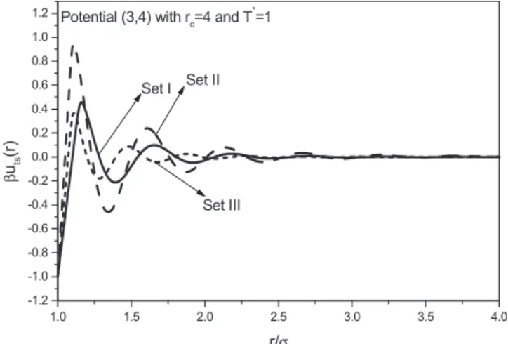
precise form of the potential and are connected with the sol-vent bath properties by means of very complicated relation-ships whose explicit mathematical form is beyond the scope of the present paper. The part for b艌r/␴艌1 reflects the depletion attraction 关35兴 induced by the finite size of the solvent particles, and the part for b⬍r/␴reflects the packing effect of the solvent particles. By properly choosing the pa-rameters, the potential共3兲 and 共4兲 not only mimics the shape of the potential arising in depletion interactions, but also other kinds of interactions, such as the effective interionic pair potentials in some alkali metals 关37兴 and alloys 关38兴. The shape of the potential共3兲 and 共4兲 is shown in Fig.1for three combinations of the potential parameters.

III. MONTE CARLO SIMULATIONS AND THERMODYNAMIC PERTURBATION THEORY

A. Monte Carlo simulations

We have performed Monte Carlo simulations in the ca-nonical共NVT兲 ensemble for SW fluids with ␭=1.05 and re-duced temperatures T*⬅kT/␧=0.50 and 0.80 and for ␭

= 1.15 and reduced temperatures T*= 0.68 and 0.90 The range of reduced densities considered was␳*= 0.1– 1.0, with step 0.1, where␳*₌␳␴3 _{and␳= N/V is the number density.}

To obtain the compressibility factor Z = pV/NkT, the ex-cess energy Uex/N␧, and the constant-volume excess heat

capacity C_Vex/Nk, the system considered consisted of N = 500 particles, initially placed in a low-density fcc configu-ration. Next, the particles were allowed to move while in-creasing their diameters until the desired reduced density␳*

was achieved. Then the system was equilibrated at the de-sired reduced temperature T* _{for Ne}= 2⫻104 _{cycles, each} cycle consisting in an attempted move per particle. The ac-ceptance ratio was fixed at around 50%. The thermodynamic properties were determined from averages performed over the next Nc= 106cycles, with 100 partial averages from

which the statistical uncertainty was estimated as the stan-dard deviation. Such a considerable number of cycles were

needed in order to obtain satisfactory accuracy for the constant-volume excess heat capacity, which was determined from the fluctuations of the energy in the canonical en-semble, through the exact relationship CV=共具U2典

−具U典2_兲/kT2_{. If only the excess energy and the equation of} state were needed, a much lower number of cycles would have been sufficient. Using the simulation data for g共r兲, the compressibility factor Z was obtained from the virial equa-tion and the excess energy Uex/N␧ was determined from the

energy equation. The reduced pressure was obtained as p*

⬅p␴3_{/␧=␳*T*Z. These quantities are listed in TablesIand}

II.

To determine the excess Helmholtz free energy Fex/NkT,

we have used two procedures. The first of them, labeled共1兲 in Tables I and II, is thermodynamic integration along iso-therms, according to the expression

Fex

NkT=

冕

共Z − 1兲d␳

⬘

␳

⬘

To this end, the simulation data for the compressibility factor

Z were fitted to a suitable polynomial in terms of ␳*_{. The}

second procedure, labeled 共2兲 in the same tables, uses the exact thermodynamic relationship

␤␮ex=

Fex

NkT+ Z − 1. 共6兲

For the excess chemical potential␮exwe used the simulation

data obtained in the form described below.

Two different procedures were used to determine the ex-cess chemical potential. The first of them, labeled 共W兲 in TablesIandII, was the Widom test particle insertion method 关39兴. We took N=1372, Ne= 2⫻104, and Nc= 5⫻104.

Statis-tical uncertainty was determined as the standard deviation from 100 partial calculations performed every 500 cycles, each with Nt= 107 trial insertions.

The second procedure, labeled共TI兲 in the tables, used the exact thermodynamic relationship 关40兴

␤␮=␤␮0+

冕

␤

uexd␤

⬘

apply the preceding equation, we performed MC NVT simu-lations to obtain the excess energy Uex/N␧ for different

val-ues of␤, from 0 to 1.6 for␭=1.15 and from 0 to 2.0 for ␭ = 1.05, along each of the isochors considered. The simula-tions were carried out with N = 500, Ne= 2⫻104, and Nc= 5

⫻104_{. The simulation data for␤U}

ex/N␧ were fitted to a

suit-able polynomial in ␤ for each of the densities considered, from which the integration involved in Eq. 共7兲 was carried out. For Z0we used the equation of state derived by Kolafa

et al.关41兴 by fitting their simulation data. This equation and the simulation data in which it is based are considered the most accurate available at present. The use of the Kolafa equation for performing the thermodynamic integration of the simulation data is justified to avoid any additional source of error 共although very small兲 in the “exact” data. However,

1.0 1.5 2.0 2.5 3.0 3.5 4.0 -1.2 -1.0 -0.8 -0.6 -0.4 -0.2 0.0 0.2 0.4 0.6 0.8 1.0 1.2 Set III Set II Set I

Potential (3,4) with rc=4 and T

* =1 β uts (r ) r/σ

FIG. 1. Shape of the potential model defined by Eqs. 共3兲 and

the most simple, but still very accurate, Carnahan-Starling 共CS兲 equation 关42兴 is completely satisfactory for theoretical calculations. The chemical potential␮₀exfor the hard-sphere fluid was determined from thermodynamic integration of its equation of state, Z0, using Eqs. 共5兲 and 共6兲.

For fluids with the potential form 共3兲 and 共4兲, we have performed MC NVT simulations for three parameter sets:共a兲

b = 1.15, a = 1.0, ks= 12, n = 3, and ␧b= 0.5; 共b兲 b=1.1, a

= 0.55, ks= 12, n = 3, and ␧b= 1.0; and共c兲 b=1.1, a=0.8, ks

= 16, n = 4, and ␧b= 0.4. The shape of the potential for these

three sets of parameters is shown in Fig.1. In all simulations the cutoff distance was fixed at rc= 4. The temperatures

con-sidered were T*= 0.5, 0.8, and 1.1 for the first two sets and

T*= 0.4, 0.7, and 1.0 for the third set. In all cases the density range covered was ␳*_{= 0.1– 0.9 with step 0.1. To obtain the}

compressibility factor Z and the excess energy Uex/N␧, from

the virial and the energy equations, respectively, we took N = 500, Ne= 2⫻104, and Nc= 5⫻104. Statistical uncertainty

was determined as the standard deviation from 100 partial calculations. The reduced pressure p* was calculated from the simulation data for Z in the form indicated before. The excess Helmholtz free energy Fex/NkT was determined by

means of thermodynamic integration共TI兲 from Eq. 共5兲. The results are shown in TablesIII–V.

B. Thermodynamic perturbation theory

In the three-order TPT 关13兴, the excess Helmholtz free energy Fexof the system is given by

Fex= Fex-ref+ Fex-tail, Fex-tail=

兺

n=1 3 Fex-n, 共8兲 F_ex-n= 1 n!N2␲␳

冕

冏

冏

excess Helmholtz free energy of a reference hard-sphere fluid with a potential uref, and uper共r兲 is the perturbation part

of the whole potential u共r兲 given by

u共r兲 = uref共r兲 + uper共r兲. 共10兲

In the present form of the third-order TPT关13兴, uref共r兲 is

the hard-sphere potential given by

uref共r兲 = ⬀ , r ⬍␴,

0, r⬎␴. 共11兲

g共r,␣,␳兲 is the radial distribution function 共RDF兲 of the bulk fluid with pair potential u共r;␣兲 given by

u共r;␣兲 = uref共r兲 +␣uper共r兲. 共12兲

兩⳵共n−1兲g共r,␣,␳兲

⳵␣共n−1兲 兩␣=0is the共n−1兲th derivative evaluated at␣= 0 of

g共r,␣,␳兲 with respect to ␣, and 兩⳵0g共r,␣,␳兲_⳵␣0 兩␣=0= g共r,0,␳兲 is

TABLE I. Simulation results for the SW fluid with␭=1.05 共see explanations in the text兲. The numbers between parentheses are the statistical uncertainties in the last decimal place.

␳* Z U_ex/N␧ C_Vex/Nk p* Fex/NkT 共1兲 Fex/NkT 共2兲 ␤␮共TI兲ex ␤␮共W兲ex T*= 0.50 0.10 1.009共6兲 −0.241 0.879共5兲 0.0505共2兲 0.006 0.004 0.013 0.009 0.20 1.034共6兲 −0.481 1.57共2兲 0.1034共4兲 0.018 0.015 0.049 0.045 0.30 1.078共6兲 −0.724共1兲 1.99共3兲 0.1617共9兲 0.040 0.036 0.114 0.112共1兲 0.40 1.156共6兲 −0.970共1兲 2.29共4兲 0.231共1兲 0.072 0.067 0.223 0.219共2兲 0.50 1.281共7兲 −1.229共1兲 2.54共6兲 0.320共2兲 0.120 0.117 0.398 0.388共3兲 0.60 1.460共8兲 −1.510共1兲 2.54共5兲 0.438共2兲 0.185 0.184 0.644 0.635共5兲 0.70 1.71共1兲 −1.809共1兲 2.62共7兲 0.599共4兲 0.27 0.27 0.98 0.98共1兲 0.80 2.14共1兲 −2.151共1兲 2.46共6兲 0.856共4兲 0.39 0.39 1.53 1.50共3兲 0.90 2.89共1兲 −2.551共1兲 2.33共6兲 1.300共5兲 0.57 0.54 2.43 2.37共5兲 1.00 4.20共3兲 −3.021共2兲 1.84共4兲 2.10共2兲 0.83 0.81 4.01 T*= 0.80 0.10 1.146共3兲 −0.122 0.174 0.0917共2兲 0.141 0.135 0.281 0.275 0.20 1.319共5兲 −0.260 0.339共1兲 0.2110共8兲 0.293 0.285 0.604 0.600 0.30 1.529共5兲 −0.415 0.488共2兲 0.367共1兲 0.461 0.453 0.982 0.988共1兲 0.40 1.823共5兲 −0.593 0.629共4兲 0.583共2兲 0.651 0.644 1.467 1.464共1兲 0.50 2.200共6兲 −0.799 0.742共6兲 0.880共2兲 0.872 0.868 2.068 2.055共2兲 0.60 2.675共6兲 −1.038 0.833共9兲 1.284共3兲 1.131 1.128 2.803 2.811共4兲 0.70 3.382共7兲 −1.319 0.94共1兲 1.894共4兲 1.441 1.441 3.823 3.811共7兲 0.80 4.394共9兲 −1.656 0.95共1兲 2.812共6兲 1.819 1.813 5.207 5.20共2兲 0.90 5.87共1兲 −2.062共1兲 0.96共2兲 4.223共7兲 2.30 2.29 7.16 7.12共8兲 1.00 8.28共2兲 −2.567共1兲 0.89共2兲 6.62共2兲 2.93 2.91 10.19

the RDF of the hard-sphere fluid with density␳and diameter

␴.

On the other hand, the excess Helmholtz free energy in second-order MCA TPT关12兴 is given by

Fex= Fex-ref+ Fex-tail= Fex-ref+ N2␲␳

冕

− N␤2␲␳

冕

冉

冊

The RDF g共r,␣,␳兲 was obtained by solving the Ornstein-Zernike 共OZ兲 integral equation theory 共IET兲 approximating the bridge function by an accurate expression for the hard-sphere fluid developed by Malijevský and Labík 关43兴. This approximation is based on the fact that we are interested in the region␣ close to 0, where it is expected that the bridge function will not be very different from that corresponding to the reference hard-sphere fluid. The derivatives

兩⳵共n−1兲g共r,␣,␳兲

⳵␣共n−1兲 兩␣=0for n = 1 , 2 , 3 were calculated numerically by

finite differences. Fex-ref and the compressibility

1

␤共⳵P⳵␳兲ref of

the reference hard-sphere fluid are calculated by means of the CS equation of state关42兴. The Verlet-Weis expression for

g共r,0,␳兲 关44兴 was used in Eq. 共13兲. The reader can consult Ref. 关13兴 for further details.

After determining Fex/NkT, the other thermodynamic

quantities are obtained by simple differentiation

manipula-tion. Thus, the reduced excess chemical potential ␤␮ex is

given by

␤␮ex=

冉

⳵共␳*␤_Fex/NkT兲

⳵␳*

冊

from which the reduced pressure P*= P␴3_{/␧ immediately} follows:

P*_{= P}␴3_{/␧ =␤␮␳*T*−␤f␳*T*, 共15兲} where␤␮=␤␮ex+ ln␳*and␤f = Fex/NkT+ln␳*− 1.

The reduced excess energy Uex/N␧ is obtained in the form

Uex/N␧ = − T*2

冋

⳵共Fex/NkT兲

T*

册

which in turn allows us to obtain the reduced constant-volume excess heat capacity C_Vex/Nk:

CV

ex_{/Nk =}

冋

⳵T*

册

IV. RESULTS FOR SHORT-RANGED SQUARE-WELL FLUIDS

The results from the second-order MCA TPT and the third-order TPT for the thermodynamic properties of

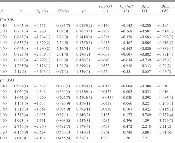
short-TABLE II. Simulation results for the SW fluid with␭=1.15 共see explanations in the text兲. The numbers between parentheses are the statistical uncertainties in the last decimal place.

␳* Z U_ex/N␧ C_Vex/Nk p* Fex/NkT 共1兲 Fex/NkT 共2兲 ␤␮共TI兲ex ␤␮共W兲ex T*= 0.68 0.10 0.863共3兲 −0.457 0.994共7兲 0.0587共2兲 −0.140 −0.143 −0.280 −0.285 0.20 0.761共3兲 −0.880 1.69共3兲 0.1035共4兲 −0.269 −0.268 −0.507 −0.514共1兲 0.30 0.695共3兲 −1.264共1兲 2.08共3兲 0.1418共6兲 −0.381 −0.378 −0.683 −0.692共2兲 0.40 0.657共3兲 −1.629共2兲 2.24共5兲 0.1787共8兲 −0.473 −0.462 −0.805 −0.816共2兲 0.50 0.662共4兲 −1.980共2兲 2.10共5兲 0.225共1兲 −0.549 −0.542 −0.880 −0.889共4兲 0.60 0.725共5兲 −2.339共1兲 2.01共4兲 0.296共2兲 −0.607 −0.607 −0.882 −0.871共7兲 0.70 0.895共6兲 −2.729共1兲 1.68共4兲 0.426共3兲 −0.640 −0.634 −0.739 −0.75共1兲 0.80 1.285共8兲 −3.176共1兲 1.38共3兲 0.699共4兲 −0.632 −0.628 −0.343 −0.29共2兲 0.90 2.19共1兲 −3.703共1兲 0.97共1兲 1.339共6兲 −0.55 −0.55 0.637 0.63共5兲 T*= 0.90 0.10 0.998共1兲 −0.327 0.360共1兲 0.0898共1兲 −0.0188 −0.004 −0.006 −0.010 0.20 1.020共2兲 −0.648 0.620共4兲 0.1836共4兲 −0.0133 0.003 0.023 0.016 0.30 1.072共2兲 −0.970 0.792共7兲 0.2894共5兲 0.00354 0.020 0.092 0.085共1兲 0.40 1.161共3兲 −1.303 0.896共9兲 0.418共1兲 0.0339 0.060 0.221 0.208共1兲 0.50 1.316共3兲 −1.654 0.895共9兲 0.592共1兲 0.0850 0.107 0.423 0.415共2兲 0.60 1.572共4兲 −2.035 0.87共1兲 0.849共2兲 0.165 0.177 0.749 0.737共4兲 0.70 1.995共4兲 −2.461 0.808共8兲 1.257共3兲 0.282 0.296 1.291 1.274共7兲 0.80 2.746共5兲 −2.950 0.692共7兲 1.977共4兲 0.458 0.472 2.218 2.21共2兲 0.90 4.133共9兲 −3.524 0.580共7兲 3.348共7兲 0.734 0.748 3.881 3.81共6兲 1.00 7.01共3兲 −4.197 0.455共5兲 6.31共3兲 1.20 1.20 7.21

ranged square well fluids are compared in Figs.2–6with the simulation data of TablesIandII. Two facts emerge clearly from these figures:共a兲 the third-order TPT provides excellent agreement with simulation data, even at low temperatures, for all the thermodynamic properties considered, but in some cases for the constant volume excess heat capacity CV

ex_/Nk,

and共b兲 the third-order TPT constitutes a strong improvement over the second-order TPT-MCA

The fact that the second-order MCA TPT provides poorer agreement with the simulation data for the excess energy as the potential width ␭ becomes shorter, as seen in Fig. 6, is due to the fact that the relative importance of the higher-order perturbative terms increases as the potential width is reduced. Moreover, the MCA strongly underestimates the magnitude of the second-order perturbative term of the Helmholtz free energy, which is directly related to the corre-sponding term of the excess energy, for short-ranged SW potentials关45兴.

Another drawback of the second-order MCA TPT, also seen in Fig. 6, is that the predicted temperature dependence of the excess energy is too small. This is reflected in the poor prediction of the constant-volume excess heat capacity shown in Fig. 3.

In contrast, the fact that the third-order TPT provides very good agreement with the simulation data for the excess en-ergy, even for short-ranged SW potentials, not only is due to include the third-order perturbative term, but also implies that the prediction of the second-order term by this theory is good. Now, the temperature dependence of Uex/N␧ is more

accurately reproduced. As a consequence, this theory pre-dicts values of C_Vex/Nk in much closer agreement with simu-lation data than those from the second-order MCA TPT, as seen in Fig.3. However, to achieve complete accuracy with simulation data for CV

ex_{/Nk, it would be necessary the}

incor-poration of higher-order perturbative terms.

One might argue that we are comparing a second-order TPT with a third-order one and that, if the Barker-Henderson

TABLE III. Simulation results for a fluid with the model poten-tial共3兲 and 共4兲 with the first parameter set.

␳* Z Uex/N␧ p* Fex/NkT T*= 0.5 0.10 1.08共2兲 −0.161 0.0539共8兲 0.09 0.20 1.19共2兲 −0.329共1兲 0.119共2兲 0.17 0.30 1.31共2兲 −0.511共1兲 0.196共3兲 0.27 0.40 1.50共2兲 −0.708共1兲 0.300共4兲 0.38 0.50 1.78共3兲 −0.923共2兲 0.446共7兲 0.53 0.60 2.12共3兲 −1.159共2兲 0.64共1兲 0.70 0.70 2.61共4兲 −1.433共2兲 0.91共1兲 0.90 0.80 3.33共5兲 −1.732共2兲 1.33共2兲 1.16 0.90 4.68共7兲 −2.093共2兲 2.11共3兲 1.51 T*= 0.8 0.10 1.171共8兲 −0.090 0.0937共6兲 0.162 0.20 1.40共1兲 −0.194 0.223共2兲 0.34 0.30 1.65共2兲 −0.314 0.395共4兲 0.55 0.40 2.03共1兲 −0.454 0.649共5兲 0.79 0.50 2.49共2兲 −0.620 0.996共7兲 1.06 0.60 3.12共2兲 −0.815共1兲 1.499共9兲 1.39 0.70 4.04共3兲 −1.044共1兲 2.26共2兲 1.78 0.80 5.18共3兲 −1.313共2兲 3.313共2兲 2.26 0.90 6.80共5兲 −1.645共2兲 4.893共3兲 2.84 T*= 1.1 0.10 1.207共5兲 −0.0651 0.1328共6兲 0.204 0.20 1.44共1兲 −0.143 0.318共2兲 0.42 0.30 1.79共1兲 −0.237 0.591共4兲 0.66 0.40 2.25共1兲 −0.350 0.992共6兲 0.95 0.50 2.81共2兲 −0.485 1.545共9兲 1.28 0.60 3.53共2兲 −0.652 2.33共1兲 1.67 0.70 4.56共2兲 −0.854共1兲 3.51共2兲 2.14 0.80 6.04共3兲 −1.107共2兲 5.31共3兲 2.71 0.90 8.04共4兲 −1.426共2兲 7.96共4兲 3.41

TABLE IV. Simulation results for a fluid with the model poten-tial共3兲 and 共4兲 with the second parameter set.

␳* Z Uex/N␧ p* Fex/NkT T*= 0.5 0.10 1.12共2兲 −0.226 0.0558共9兲 0.102 0.20 1.31共2兲 −0.452共1兲 0.131共2兲 0.235 0.30 1.53共2兲 −0.686共1兲 0.230共3兲 0.400 0.40 1.92共3兲 −0.932共1兲 0.385共6兲 0.604 0.50 2.37共3兲 −1.201共2兲 0.593共8兲 0.858 0.60 3.19共4兲 −1.496共2兲 0.96共1兲 1.18 0.70 4.25共7兲 −1.816共3兲 1.49共2兲 1.58 0.80 5.52共8兲 −2.145共3兲 2.21共3兲 2.10 0.90 7.5共1兲 −2.519共3兲 3.39共5兲 2.7 T*= 0.8 0.10 1.225共8兲 −0.131 0.0980共6兲 0.212 0.20 1.55共2兲 −0.271 0.248共3兲 0.457 0.30 1.87共2兲 −0.425 0.449共3兲 0.74 0.40 2.40共2兲 −0.591 0.768共8兲 1.06 0.50 3.16共2兲 −0.770共1兲 1.263共8兲 1.45 0.60 4.03共3兲 −0.962共1兲 1.94共1兲 1.91 0.70 5.41共3兲 −1.178共2兲 3.03共2兲 2.48 0.80 7.07共5兲 −1.411共3兲 4.52共3兲 3.17 0.90 9.39共7兲 −1.699共4兲 6.76共5兲 4.02 T*= 1.1 0.10 1.256共5兲 −0.091 0.1382共6兲 0.2440 0.20 1.565共9兲 −0.189 0.344共2兲 0.5130 0.30 2.00共1兲 −0.298 0.658共5兲 0.817 0.40 2.57共2兲 −0.416 1.130共8兲 1.17 0.50 3.3130 −0.541 1.82共1兲 1.58 0.60 4.34共2兲 −0.673共1兲 2.86共1兲 2.06 0.70 5.76共2兲 −0.817共2兲 4.44共2兲 2.63 0.80 7.62共3兲 −0.989共2兲 6.71共3兲 3.31 0.90 10.05共5兲 −1.191共3兲 9.95共5兲 4.13

perturbation theory were extended to third or higher order, the differences between the two theories would be reduced. Such an extension is possible, because the procedure devel-oped by Barker and Henderson to obtain the second-order perturbative contribution to the free energy in the macro-scopic compressibility approximation was generalized 关46,47兴 to higher-order terms and the resulting infinite per-turbative series was summed up to obtain a closed expression for the excess Helmholtz free energy. However, the differ-ence between the results obtained in this way and those re-sulting from the perturbative series truncated at the level of the second-order term are nearly negligible. On the other hand, instead of the macroscopic compressibility approxima-tion we could have used the local compressibility approxi-mation共LCA兲 关12兴 for the second-order term in the Barker-Henderson TPT. However, at least for SW fluids, the difference between the two approximations is small关19,45兴. In Figs. 2–6 it seems that the relative accuracy of the third-order TPT increases as the well width decreases, and

this becomes more apparent in Fig. 3. However, it is to be noted that, from recent simulations关48兴, the reduced critical temperatures for ␭=1.05 and for ␭=1.15 are T_c*= 0.366 and

T_c*⬇0.57, respectively. Therefore, the lowest reduced

tem-perature considered for ␭=1.05 is more supercritical than that for␭=1.15, and the same is true for the highest tempera-tures considered in the two cases. This explains what at first sight may appear quite surprising. It is worth mentioning here that the liquid-vapor coexistence becomes mestastable with respect to solid-gas coexistence for ␭ of the order of 1.25 or lower关48兴.

The fact that the third-order TPT accurately predicts the pressure and the chemical potential for short-ranged SW flu-ids suggests that it might be useful for predicting the liquid-vapor coexistence. For the reasons just pointed out, it is dif-ficult to obtain reliable simulation data for the coexistence curve below␭=1.25. Therefore, we have considered two in-termediate ranges—namely,␭=1.25 and ␭=1.375.

In the third-order TPT, the coexistence curve is obtained by equating chemical potentials and pressures in both phases at a given temperature. These quantities are easily deter-mined from the total free energy. The solution of the

equi-TABLE V. Simulation results for a fluid with the model poten-tial共3兲 and 共4兲 with the third parameter set.

␳* Z Uex/N␧ p* Fex/NkT T*= 0.4 0.10 1.06共2兲 −0.153 0.042共1兲 0.051 0.20 1.12共2兲 −0.311共1兲 0.089共2兲 0.111 0.30 1.24共3兲 −0.475共1兲 0.149共3兲 0.182 0.40 1.38共3兲 −0.648共2兲 0.222共5兲 0.265 0.50 1.55共4兲 −0.834共2兲 0.310共7兲 0.367 0.60 1.82共3兲 −1.039共2兲 0.436共8兲 0.495 0.70 2.34共4兲 −1.275共2兲 0.66共1兲 0.657 0.80 2.87共6兲 −1.538共2兲 0.92共2兲 0.866 0.90 3.72共8兲 −1.850共2兲 1.34共3兲 1.13 T*= 0.7 0.10 1.157共9兲 −0.068 0.0810共6兲 0.1145 0.20 1.42共2兲 −0.147 0.201共2兲 0.303 0.30 1.70共2兲 −0.242 0.357共3兲 0.527 0.40 2.02共2兲 −0.352 0.565共6兲 0.775 0.50 2.48共2兲 −0.484 0.868共7兲 1.05 0.60 3.13共2兲 −0.643共1兲 1.32共1兲 1.37 0.70 4.06共3兲 −0.835共1兲 1.99共2兲 1.76 0.80 5.31共4兲 −1.064共1兲 2.97共2兲 2.25 0.90 7.11共5兲 −1.352共2兲 4.48共3兲 2.86 T*= 1.0 0.10 1.207共6兲 −0.046 0.1207共6兲 0.2036 0.20 1.46共1兲 −0.103 0.291共2兲 0.420 0.30 1.79共1兲 −0.173 0.538共4兲 0.664 0.40 2.21共2兲 −0.259 0.885共6兲 0.948 0.50 2.83共2兲 −0.365 1.415共9兲 1.28 0.60 3.60共2兲 −0.497 2.16共1兲 1.68 0.70 4.68共2兲 −0.664共1兲 3.28共2兲 2.16 0.80 6.20共3兲 −0.869共1兲 4.96共3兲 2.74 0.90 8.37共4兲 −1.137共2兲 7.53共3兲 3.47 0.2 0.4 0.6 0.8 1.0 -1 0 1 2 3 4 5 6 7 8 9 10 11 12 T*=0.8 T*=0.5 λ=1.05 βµex ρ* 0.2 0.4 0.6 0.8 1.0 -1 0 1 2 3 4 5 6 7 8 T*=0.9 T*=0.68 λ=1.15 βµex ρ*

FIG. 2. Excess chemical potential for the square-well fluids con-sidered. Points: simulation data from TablesI andII. Squares and solid circles, nearly indistinguishable from each other at the scale of the figure, correspond to TI and W procedures, respectively. Dashed curves: Barker-Henderson second-order MCA TPT. Solid curves: Zhou third-order TPT.

librium conditions corresponds to a double-tangent construc-tion on the curve of the free energy per unit volume versus the density. To this end, the free energy curve is obtained numerically at different temperatures. As the numerical implementation of the third-order TPT involves the calcula-tion of g共r,␣,␳兲 corresponding to the pair potential u共r;␣兲 given by Eq.共12兲, then one might think that a problem would be the possible breakdown of the code when the considered temperature is below the critical temperature. Such a prob-lem actually does not arises because, to obtain numerically the derivatives 兩⳵共n−1兲g共r,␣,␳兲/⳵␣共n−1兲兩_␣=0 with n = 1 , 2 , 3, involved in Eq.共9兲, one only needs to calculate the values of

g共r,␣,␳兲 for ␣= 0 ,⫾⌬␰,⫾2⌬␰, where ⌬␰ is a small quantity—for example, 0.005. For such small values of ␣,

u共r;␣兲 is very close to the hard-sphere potential or,

equiva-lently, very close to the infinite-temperature limit. Therefore, the calculations of the perturbative terms are performed at a temperature that is always much higher than the critical tem-perature of the true potential u共r兲. This is exactly why we can use the hard-sphere bridge function for the potential

u共r;␣兲 when␣is very small, as we mentioned before. From another viewpoint, solving the OZ integral equation for

u共r;␣兲 at temperature T is actually equivalent to solving the

OZ integral equation for u共r兲 at temperature T/␣. When␣is sufficiently small, the equivalent temperature T/␣ for the

potential u共r兲 is sufficiently high and always higher than the critical temperature of the potential u共r兲.

The results for the liquid-vapor coexistence obtained from the third-order TPT and those from the Barker-Henderson second-order TPT in the MCA are compared in Fig. 7 with the simulation data 关49–51兴. We have included for compari-son the results from the self-consistent OZ approximation 共SCOZA兲, recently extended to SW fluids 关52兴, although it belongs to a different class of theories. The figure shows that the third-order TPT compares favorably with the other two theories.

V. RESULTS FOR THE OSCILLATORY POTENTIAL MODEL

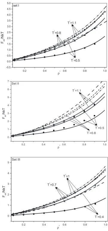
In Figs.8–10, the results from the two perturbation theo-ries for the thermodynamic properties of fluids with interpar-ticle interactions obeying to the oscillatory potential 共3兲 and 共4兲 are compared with the simulation data from TablesIII–V. The same conclusions can be drawn about the relative per-formance of both perturbation theories. Now, the superior quality of the third-order TPT over the second-order MCA TPT is particularly noteworthy for the excess energy, as

0.2 0.4 0.6 0.8 1.0 0.0 0.4 0.8 1.2 1.6 2.0 2.4 2.8 T*=0.8 T*=0.5 λ=1.05 CV e x /Nk ρ* 0.2 0.4 0.6 0.8 1.0 -0.5 0.0 0.5 1.0 1.5 2.0 2.5 T*=0.9 T*=0.68 λ=1.15 CV ex /Nk ρ*

FIG. 3. Constant-volume excess heat capacity for square-well fluids. Points: simulation data from TablesIandII. The curves have the same meaning as in Fig.2.

0.2 0.4 0.6 0.8 1.0 -1.0 -0.5 0.0 0.5 1.0 1.5 2.0 2.5 3.0 3.5 T*=0.8 T*=0.5 λ=1.05 Fex /Nk T ρ* 0.2 0.4 0.6 0.8 1.0 -0.8 -0.4 0.0 0.4 0.8 1.2 1.6 T*=0.9 T*=0.68 λ=1.15 Fex /Nk T ρ*

FIG. 4. Excess Helmholtz free energy for the square-well fluids considered. Points: data from Tables I and II. Squares and solid circles, nearly indistinguishable from each other at the scale of the figure, correspond to procedures 共1兲 and 共2兲, respectively. The curves have the same meaning as in Fig.2.

shown in Fig. 10. In this figure stands out a quality also present, but less clearly, in Fig.6for the excess energy of the SW fluid—namely, the fact that the third-order TPT clearly differentiates the energy of isotherms with temperatures close to each other. In contrast, the second-order MCA TPT does not. This is because, as pointed before, in the latter theory the second-order term in the energy, from which de-pends the variation with temperature of the excess energy,

Uex/N␧, is usually very small.

In the previous section we have pointed out that the third-order TPT seems accurate enough so as to provide reliable estimates of the liquid-vapor coexistence. Thus, we have used it to estimate the critical temperatures for the three sets of parameters considered for the oscillatory potential共3兲 and 共4兲. They are T_c*= 0.3365, 0.3692, and 0.2989 for sets I, II, and III, respectively. Therefore, the lowest temperature con-sidered in the simulations and the theoretical calculations for each of the three sets is higher than, but close to, the critical temperature.

However, it is to be noted that, among the three sets of parameters considered, the third-order TPT, in combination with a first-order TPT关53兴 for the solid phase, only predicts a stable liquid phase for set II. For the two other sets of parameters, the liquid-vapor coexistence is metastable with respect to the solid-gas coexistence.

0.2 0.4 0.6 0.8 1.0 0 1 2 3 4 5 6 7 T*=0.8 T*=0.5 λ=1.05 P σ 3 /ε ρ* 0.2 0.4 0.6 0.8 1.0 0 1 2 3 4 5 6 7 T*=0.9 T*=0.68 λ=1.15 P σ 3 /ε ρ*

FIG. 5. Reduced pressure for the square-well fluids considered. Points: data from TablesIandII. The curves have the same mean-ing as in Fig.2. 0.2 0.4 0.6 0.8 1.0 -3.5 -3.0 -2.5 -2.0 -1.5 -1.0 -0.5 0.0 0.5 T*=0.8 T*=0.5 λ=1.05 Uex /N ε ρ* 0.2 0.4 0.6 0.8 1.0 -4.5 -4.0 -3.5 -3.0 -2.5 -2.0 -1.5 -1.0 -0.5 0.0 0.5 T*=0.9 T*=0.68 λ=1.15 Uex /N ε ρ*

FIG. 6. Reduced excess energy for the square-well fluids con-sidered. Points: simulation data from Tables I and II. The curves have the same meaning as in Fig.2.

0.0 0.1 0.2 0.3 0.4 0.5 0.6 0.7 0.8 0.9 0.5 0.6 0.7 0.8 0.9 1.0 1.1 λ=1.25 λ=1.375 T * ρ*

FIG. 7. Liquid-vapor coexistence for square-well fluids. Points are the simulation data from Refs. 关49–51兴, respectively, for

squares, triangles, and diamonds. Solid lines are the results from the third-order TPT, dashed lines are the results from the SCOZA关52兴,

and the short-dashed lines are the results from the second-order MCA TPT.

It has been shown 关54–56兴 that in models of colloidal fluids with short-range attractive and weak long-range repul-sive competing interactions, a microphase separation can take place, with large stabilized clusters, at temperatures be-low the critical temperature, preventing gas-liquid separa-tion. This situation is not present in the states we have stud-ied for the oscillatory potential, because all the temperatures considered are supercritical. In any case, with the sets of

parameters considered it is not expected that a stable mi-crophase separation will occur even at subcritical tempera-tures, because the repulsive interactions, apart from the hard core, are not enough weak nor long ranged. Moreover, the long-range oscillatory tail of the potential hinders the forma-tion of such microphases.

VI. CONCLUSIONS

In the preceding sections we have provided compelling evidence of the great accuracy of the third-order

thermody-0.2 0.4 0.6 0.8 1.0 -0.5 0.0 0.5 1.0 1.5 2.0 2.5 3.0 3.5 4.0 4.5 5.0 T*=1.1 T*=0.8 T*=0.5 set I Fex /N kT ρ* 0.2 0.4 0.6 0.8 1.0 0 1 2 3 4 5 6 7 T* =1.1 T* =0.8 T* =0.5 Set II Fex /N kT ρ* 0.2 0.4 0.6 0.8 1.0 0 1 2 3 4 5 T*=1 T*=0.7 T*=0.4 Set III Fex /NkT ρ*

FIG. 8. Excess Helmholtz free energy for fluids with the oscil-latory potential共3兲 and 共4兲. Points: data from TablesIII–V. Dashed curves: Barker-Henderson second-order perturbation theory in the MCA. Solid curves: third-order TPT of this work.

0.2 0.4 0.6 0.8 1.0 0 2 4 6 8 10 T*=1.1 T*=0.8 T*=0.5 Set I P σ 3 /ε ρ* 0.2 0.4 0.6 0.8 1.0 0 2 4 6 8 10 12 14 T*=1.1 T*=0.8 T*=0.5 Set II P σ 3 /ε ρ* 0.2 0.4 0.6 0.8 1.0 0 2 4 6 8 10 12 14 T*=1 T*=0.7 T*=0.4 Set III P σ 3 /ε ρ*

namic perturbation theory 关13兴, summarized in Sec. III, for most of the thermodynamic properties considered. In fact, this theory is much more accurate than the second-order Barker-Henderson perturbation theory in the MCA.

The reasons why the performance of the third-order TPT is superior to that of the Barker-Henderson 共BH兲 second-order TPT are quite obvious: on the one hand, the BH per-turbation theory predicts values for the second-order pertur-bative term in the energy that are too small in magnitude, especially for short-ranged potentials, as shown in Ref.关45兴, whereas the second-order term in the third-order TPT is much more accurate关13兴. This is due to the fact that, in the latter, the second-order term is associated with the first-order derivative of the radial distribution function g共r,␣,␳兲 evalu-ated at ␣= 0, as required rigorously by the TPT, whereas in the BH second-order TPT the same term is evaluated from the RDF g共r,0,␳兲 of the reference fluid, which is a more crude approximation. On the other hand, the third-order TPT includes an additional term, and it is known that higher-order terms become increasingly important with decreasing poten-tial range, temperature, and density. In contrast, adding higher-order terms to the BH TPT in the MCA does not result in any significant improvement, as they are nearly neg-ligible.

From the preceding considerations, we can conclude that the performance of the third-order perturbation theory devel-oped by one of us 关13,14兴 in predicting the thermodynamic properties of fluids with short-ranged and oscillatory poten-tials is very satisfactory. This makes it particularly suitable to deal with complex fluids and colloidal suspensions. A re-markable fact is that the theory is particularly accurate for the pressure and the excess chemical potential, two quantities that play an essential role in studying phase transitions.

For the constant-volume excess heat capacity C_Vex/Nk in-stead, the third-order TPT is still insufficient to provide enough accuracy at very low temperatures and higher-order terms would be needed.

ACKNOWLEDGMENTS

J.R.S. acknowledges financial support under Grant No. MERG-CT-2007-046453. This project is supported by the National Natural Science Foundation of China 共Grant No. 20673150兲.

关1兴 N. Willenbacher and C. Oelschlaeger, Curr. Opin. Colloid In-terface Sci. 12, 43共2007兲.

关2兴 J. Largo and N. B. Wilding, Phys. Rev. E 73, 036115 共2006兲. 关3兴 E. Bianchi, J. Largo, P. Tartaglia, E. Zaccarelli, and F.

Scior-tino, Phys. Rev. Lett. 97, 168301共2006兲.

关4兴 S. Brandon, P. Katsonis, and P. G. Vekilov, Phys. Rev. E 73,

061917共2006兲.

关5兴 A. J. Archer, D. Pini, R. Evans, and L. Reatto, J. Chem. Phys.

126, 014104共2007兲.

关6兴 G. Cinacchi, Y. Martínez-Ratón, L. Mederos, G. Navascués, A. Tani, and E. Velasco, J. Chem. Phys. 127, 214501共2007兲. 关7兴 J. Largo, P. Tartaglia, and F. Sciortino, Phys. Rev. E 76,

0.2 0.4 0.6 0.8 1.0 -2.5 -2.0 -1.5 -1.0 -0.5 0.0 Set I T*=1.1 T*_=0.8 T*_=0.5 Uex /N ε ρ* 0.2 0.4 0.6 0.8 1.0 -3.0 -2.5 -2.0 -1.5 -1.0 -0.5 0.0 0.5 1.0 T*=1.1 T*=0.8 T*=0.5 Set II Uex /N ε ρ* 0.2 0.4 0.6 0.8 1.0 -3.0 -2.5 -2.0 -1.5 -1.0 -0.5 0.0 0.5 Set III T*=1 T*=0.7 T*=0.4 Uex /N ε ρ*

011402共2007兲.

关8兴 A. Matsuyama and R. Hirashima, J. Chem. Phys. 128, 044907 共2008兲.

关9兴 A. J. Rahedi, J. F. Douglas, and F. J. Starr, J. Chem. Phys. 128, 024902共2008兲.

关10兴 P. R. Lang, J. Chem. Phys. 127, 124906 共2007兲; A. R. Herring and J. R. Henderson, Phys. Rev. E 75, 011402共2007兲; J. R. Henderson, ibid. 73, 010402共R兲 共2006兲; P. Melby, A. Prevost, D. A. Egolf, and J. S. Urbach, ibid. 76, 051307共2007兲. 关11兴 R. Roth and M. Kinoshita, J. Chem. Phys. 125, 084910

共2006兲; D. Gazzillo, A. Giacometti, R. Fantoni, and P. Sollich, Phys. Rev. E 74, 051407共2006兲.

关12兴 J. A. Barker and D. Henderson, J. Chem. Phys. 47, 2856 共1967兲.

关13兴 S. Zhou, Phys. Rev. E 74, 031119 共2006兲. 关14兴 S. Zhou, J. Phys. Chem. B 111, 10736 共2007兲.

关15兴 D. Henderson, O. H. Scalise, and W. R. Smith, J. Chem. Phys.

72, 2431共1980兲.

关16兴 D. M. Heyes and P. J. Aston, J. Chem. Phys. 97, 5738 共1992兲. 关17兴 J. Largo and J. R. Solana, Phys. Rev. E 67, 066112 共2003兲. See also the supplementary material to this paper, EPAPS Docu-ment No.E-PLEEE8-67-132306. This docuDocu-ment may be ac-cessed from the reference section of the online article, or via the EPAPS homepage http:/www.aip.org/pubservs/epaps.html 关18兴 A. Malijevsky, S. B. Yuste, and A. Santos, J. Chem. Phys.

125, 074507共2006兲.

关19兴 J. Largo, J. R. Solana, L. Acedo, and A. Santos, Mol. Phys.

101, 2891共2003兲.

关20兴 J.-S. Huang, S. A. Safran, M. W. Kim, G. S. Grest, M. Kotlar-chyk, and N. Quirke, Phys. Rev. Lett. 53, 592共1984兲. 关21兴 A. Lang, G. Kahl, C. N. Likos, H. Löwen, and M. Watzlawek,

J. Phys.: Condens. Matter 11, 10143共1999兲.

关22兴 E. Zaccarelli, G. Foffi, K. A. Dawson, F. Sciortino, and P. Tartaglia, Phys. Rev. E 63, 031501共2001兲.

关23兴 K. Dawson, G. Foffi, M. Fuchs, W. Götze, F. Sciortino, M. Sperl, P. Tartaglia, Th. Voigtmann, and E. Zaccarelli, Phys. Rev. E 63, 011401共2000兲.

关24兴 L. Acedo and A. Santos, J. Chem. Phys. 115, 2805 共2001兲. 关25兴 G. Foffi, K. A. Dawson, S. V. Buldyrev, F. Sciortino, E.

Zac-carelli, and P. Tartaglia, Phys. Rev. E 65, 050802共R兲 共2002兲. 关26兴 G. Foffi, G. D. McCullagh, A. Lawlor, E. Zaccarelli, K. A.

Dawson, F. Sciortino, P. Tartaglia, D. Pini, and G. Stell, Phys. Rev. E 65, 031407共2002兲.

关27兴 E. Zaccarelli, G. Foffi, K. A. Dawson, S. V. Buldyrev, F. Sci-ortino, and P. Tartaglia, J. Phys.: Condens. Matter 15, S367 共2003兲.

关28兴 C. F. Tejero, J. F. Lutsko, J. L. Colot, and M. Baus, Phys. Rev. A 46, 3373共1992兲.

关29兴 B. Davoudi, M. Kohandel, M. Mohammadi, and B. Tanatar, Phys. Rev. E 62, 6977共2000兲.

关30兴 H. Guerin, Physica A 304, 327 共2002兲.

关31兴 A. A. Louis, E. Allahyarov, H. Löwen, and R. Roth, Phys. Rev. E 65, 061407共2002兲.

关32兴 J. Serrano-Illán, G. Navascués, E. Velasco, and L. Mederos, J. Chem. Phys. 119, 1510共2003兲.

关33兴 C. Barrio and J. R. Solana, Lect. Notes Phys. 753, 133 共2008兲. 关34兴 R. Roth, R. Evans, and S. Dietrich, Phys. Rev. E 62, 5360

共2000兲.

关35兴 S. Asakura and F. Osawa, J. Chem. Phys. 22, 1255 共1954兲; A. Vrij, Pure Appl. Chem. 48, 471共1976兲.

关36兴 J. C. Crocker, J. A. Matteo, A. D. Dinsmore, and A. G. Yodh, Phys. Rev. Lett. 82, 4352共1999兲.

关37兴 J.-F. Wax, R. Albaki, and J.-L. Bretonnet, Phys. Rev. B 62, 14818共2000兲.

关38兴 J. A. Moriarty and M. Widom, Phys. Rev. B 56, 7905 共1997兲. 关39兴 B. Widom, J. Chem. Phys. 39, 2808 共1963兲.

关40兴 S. Labík, A. Malijevsky, R. Kao, W. R. Smith, and F. dell Río, Mol. Phys. 96, 849共1999兲.

关41兴 J. Kolafa, S. Labík, and A. Malijevsky, Phys. Chem. Chem. Phys. 6, 2335共2004兲.

关42兴 N. F. Carnhan and K. E. Starling, J. Chem. Phys. 51, 635 共1969兲.

关43兴 A. Malijevský and S. Labík, Mol. Phys. 60, 663 共1987兲. 关44兴 L. Verlet and J.-J. Weis, Phys. Rev. A 5, 939 共1972兲. 关45兴 J. Largo and J. R. Solana, Mol. Simul. 29, 363 共2003兲. 关46兴 E. Praestgaard and S. Toxvaerd, J. Chem. Phys. 51, 1895

共1969兲.

关47兴 S. Toxvaerd and E. Praestgaard, J. Chem. Phys. 53, 2389 共1970兲.

关48兴 J. A. Largo, M. A. Miller, and F. Sciortino, J. Chem. Phys.

128, 134513共2008兲.

关49兴 F. del Río, E. Ávalos, R. Spíndola, L. F. Rull, G. Jackson, and S. Largo, Mol. Phys. 100, 2531共2002兲.

关50兴 J. R. Elliot and L. Hu, J. Chem. Phys. 110, 3043 共1999兲. 关51兴 L. Vega, E. de Miguel, L. F. Rull, G. Jackson, and I. A.

McLure, J. Chem. Phys. 96, 2296共1992兲.

关52兴 E. Scöll-Paschinger, A. L. Benavides, and R. Castañeda-Priego, J. Chem. Phys. 123, 234513共2005兲.

关53兴 S. Zhou, J. Chem. Phys. 127, 084512 共2007兲.

关54兴 R. P. Shear and W. M. Gelbart, J. Chem. Phys. 110, 4582 共1999兲.

关55兴 J. Groenewold and W. K. Kegel, J. Phys. Chem. B 105, 11702 共2001兲.

关56兴 F. Sciortino, S. Mossa, E. Zaccarelli, and P. Tartaglia, Phys. Rev. Lett. 93, 055701共2004兲.