Modelling and State Estimation of Batteries

Texto completo

(1)UNIVERSIDAD DE VALLADOLID ESCUELA DE INGENIERIAS INDUSTRIALES Grado en Ingeniería en Organización Industrial. Modelling and State Estimation of Batteries Autor: Rodríguez Asensio, Miguel. Responsable de Intercambio en la UVa: Fernando Tadeo Rico Universidad de destino: Université de Picardie Jules Verne - Amiens. Valladolid, Julio 2016..

(2) TFG REALIZADO EN PROGRAMA DE INTERCAMBIO. TÍTULO:. Modelling and state estimation of batteries. ALUMNO:. Miguel Rodríguez Asensio. FECHA:. 28/06/2016. CENTRO:. Laboratoire MIS. TUTOR:. Prof. A. El Hajjaji. 1.

(3) Resumen En este trabajo se ha realizado un estudio sobre el modelado y la estimación de los estados de una batería de Litio principalmente, y en la parte final del mismo sobre una batería de Plomo. Este estudio se ha desarrollado simultáneamente en MapleSim, Matlab y Simulink, utilizando el algoritmo denominado Filtro de Kalman (Kalman Filter en inglés) para estimar el estado de carga (SOC) y el estado de salud (SOH) de la batería. Este algoritmo ha sido extensamente validado a lo largo del trabajo mediante simulación, y se ha llegado a demostrar su robustez contra el ruido utilizado. Por otro lado también se ha estudiado la degradación que sufre la batería en función de la temperatura de las celdas que la componen.. Palabras clave Filtro de Kalman, batería de Litio, estado de carga (SOC), estado de salud (SOH) y modelado baterías.. 2.

(4) 3.

(5) Content. Resumen ........................................................................................................................... 2 Palabras clave ................................................................................................................... 2 1 INTRODUCTION TO BATTERIES, BATTERY MODELLING AND MAPLESIM ENVIRONMENT ................................................................................................................. 6 1.1. ORIGINS OF THE BATTERIES ............................................................................... 6. 1.2. OPERATION OF A BATTERY ................................................................................ 6. 1.3. MAIN PARAMETERS OF THE BATTERY ............................................................... 7. 1.4. REQUIREMENTS OF A BATTERY FOR THE ELECTRIC VEHICLE ............................ 8. 1.5. BATTERY MODELLING ........................................................................................ 8. 1.5.1. ELECTROCHEMICAL MODELS...................................................................... 8. 1.5.2. MATHEMATICAL MODELS ........................................................................ 11. 1.5.3. ELECTRICAL EQUIVALENT CIRCUIT MODELS............................................. 11. 1.6 2. MODELLING OF A LITHIUM-ION BATTERY .............................................................. 15 2.1. 3. MAPLESIM ENVIRONMENT .............................................................................. 12 IMPLEMENTATION OF THE BATTERY MODEL IN MATLAB ENVIRONMENT..... 19. STATE OF CHARGE ESTIMATION ALGORITHM ........................................................ 27 3.1. STATE OF THE ART ........................................................................................... 27. 3.2. INTRODUCTION TO DISCRETE SIMPLE KALMAN FILTER .................................. 32. 3.2.1 STATE OF CHARGE ESTIMATION BASED ON SIMPLE KALMAN FILTER ALGORITHM FOR LITHIUM-ION BATTERIES ............................................................ 34 3.3. EXTENDED KALMAN FILTER ............................................................................. 39. 3.3.1 STATE OF CHARGE ESTIMATION BASED ON EXTENDED KALMAN FILTER ALGORITHM FOR LITHIUM-ION BATTERIES ............................................................ 40 3.4 STATE OF CHARGE ESTIMATION BASED ON KALMAN FILTER ALGORITHM FOR LITHIUM-ION BATTERIES IN SIMULINK ....................................................................... 48 4. STATE OF HEALTH ESTIMATION ALGORITHM ......................................................... 58 4.1. INTRODUCTION ................................................................................................ 58. 4.2 STATE OF HEALTH ESTIMATION BASED ON FIFTH-ORDER EXTENDED KALMAN FILTER USING DATA FROM MAPLESIM ....................................................................... 59. 4. 4.3. SOH AND SOC ESTIMATION USING FIFTH-ORDER EKF IN SIMULINK ............... 65. 4.4. MEASUREMENT OF THE STATE OF CHARGE AT DIFFERENT TEMPERATURES . 67.

(6) 4.5 COMPARATION BETWEEN THE DEGRADATION OF ONE CELL AND A REAL BATTERY WITH EIGHT CELLS ....................................................................................... 69 5. LEAD-ACID BATTERY MODELLING ........................................................................... 71 5.1. 6. STATE ESTIMATION FOR LEAD-ACID BATTERY................................................. 72. CONCLUSIONS ......................................................................................................... 76 6.1. PRESENT WORK................................................................................................ 76. 6.2. FURTHER WORK ............................................................................................... 76. ANNEX- GUIDE TO USE MAPLESIM ................................................................................. 78 HOW TO CREATE CUSTOM COMPONENTS ................................................................. 79 CREATE A SUBSYSTEM ................................................................................................ 81 USING THE SIMULINK COMPONENT BLOCK GENERATION TEMPLATE ...................... 82 REFERENCES.................................................................................................................... 86. 5.

(7) 1 INTRODUCTION TO BATTERIES, BATTERY MODELLING AND MAPLESIM ENVIRONMENT 1.1 ORIGINS OF THE BATTERIES The first battery was invented by Alessandro Volta in 1800. There are two main kinds of batteries: the primary cells which, once they had been used, they cannot be recharged, and secondary cells which can be used many times thanks to their capacity of recharging when you supply an external current [1]. In Table 1 it is shown a classification with several examples of both kinds of batteries [2].. Primary Cells. Secondary Cells. Zinc Carbon Alkaline Lithium. Sealed Lead Acid Nickel Cadmium Nickel Metal-Hydride Lithium-ion Lithium-Polymer Table 1.- Classification of different battery types in primary or secondary cells For instance, silver coin or button cell batteries are lithium batteries since they are composed of lithium metal and, due to their irreversible chemical reaction, they are classified as primary cells. Also the well-known alkaline batteries, which can be easily found on store shelves, are classified into this group. The disposable nature of this kind of batteries means that there is no need of recharge control, protection circuity or fuel gauging, whereas the secondary batteries, they do need this actions in order to enhance their performance. Within this group we can found the Lithium-ion batteries, which are the ones that we are going to focus on throughout this document. This batteries are now widely used in today portable’s world. At the end of this document, we are going to study the Lead-Acid batteries too, which are classified as secondary cells and are usually used in automotive applications or fixed installation due to their large size and weight.. 1.2 OPERATION OF A BATTERY A battery is a device composed by one or more electrochemical cells that converts the chemical energy contained in its active materials directly into electric energy by means of an oxidation reduction (redox) reaction, which consists in the transfer of electrons from one material to another through an electric circuit [2]. During the discharge of a battery, it operates like in Figure 1.1.a). When both terminals of the battery are connected to an external load (in this case a bulb),. 6.

(8) electrodes flow from the anode, which is oxidized, through the external load to the cathode, which is reduced due to the flow of electrodes. The electric circuit is completed in the electrolyte by the flow of anions and cations to the anode and cathode, respectively. The electrolyte is an ionic conductor that allow the transfer of charge, as ions, inside the battery between the anode and the cathode [2].. a). b). Figure 1.1.- a) Discharge of Li-Ion Battery; b) Charge of Li-Ion Battery Source: http://www.sigmaaldrich.com/technical-documents/articles/materialmatters/ionic-liquids-for.html The operation inside the battery when charging is depicted in Figure 1.1.b). Now the current flow is inverted, with reduction occurring at the negative electrode and oxidation at the positive. To conclude, it is important to notice that the battery operation relies on the use of a pairs of metals that are capable of exchanging electrons.. 1.3 MAIN PARAMETERS OF THE BATTERY Each battery is characterised by the following parameters [1]: a) Usable power (P = V*I): It is obtained from the product of battery voltage (V) and the maximum current that it can tolerate (I). This usable power must be at least equal to the peak power so as to provide the electricity throughout all the operating range. b) Stored Energy (KWh): This parameter is going to determine the autonomy of the electric vehicle (EV) and the possibilities of recovering for a hybrid electric vehicle (HEV). The energy of the battery is expressed as a function of its capacity in ampere-hour (Ah) and its voltage.. 7.

(9) c) State of charge of the battery (SOC): One possible definition of the state of charge (SOC) could be the ratio of the remaining charge of the battery and the total charge while the battery is fully charged at the same specific standard condition. The SOC is often expressed in percentage, where 100% means fully charged and 0% means fully discharged [3].. 1.4 REQUIREMENTS OF A BATTERY FOR THE ELECTRIC VEHICLE The weight and volume of the batteries are some of the most important factors when choosing a battery. The electric vehicle (EV) must have a battery that meets the following requirements among others [1]: a) A good mass energy (Wh/Kg): the quantity of energy stored per mass unit. It allows to define the autonomy of the battery. b) A good power-to-weight ratio (W/Kg): The power delivered by a unit of mass of the battery. c) A steady voltage which generate a regular performance. d) A good autonomy. e) A maximum battery lifespan, expressed in number of cycles (charge/discharge) that it can support. Battery lifespan is defined as the number of times that the battery can be restored until a level of energy superior to 80% of its nominal energy. f) Less maintenance g) Availability. 1.5 BATTERY MODELLING Research in the field of electric vehicle simulation, energy distribution and power control strategy, as well as in the estimation of batteries state of charge (SOC) and state of health (SOH) is experiencing an important increase. This growing interest in this field caused that the improvement of battery models accuracy, especially those concerning Lithium-ion batteries, has become a crucial objective. This is the reason why in the literature there is a wide range of different approaches regarding the representation of battery behaviour using models with different degrees of complexity. Since the battery is a nonlinear system, the models usually used in electric vehicles can be classified into three different kinds:. 1.5.1 ELECTROCHEMICAL MODELS. 8.

(10) It is possible to achieve a high accuracy by using electrochemical models that aim to capture all the key behaviours of the battery. They are suitable for understanding the distributed electrochemistry reactions in the electrodes (such as, the reactions from Figure 1.2, assuming LiyCoO2 cathode and LixC6 anode) and electrolyte. However, in order to describe the battery chemistry charge/discharge carrier mechanisms, they deploy a high number of partial differential equations (PDEs) with a large number of unknown parameters (see from equation ( 1.1 ) to ( 1.5 )), which must be solved simultaneously with a high computational expense and a significant requirement of memory. In addition, they frequently run into over-fitting problems due to their poor model robustness under extrapolation [4], which generally precludes their use in real-time online control [5].. This kind of battery modelling tries to describe all the details of physics phenomenon that happens inside the battery. Figure 1.2 shows the anatomy of a Lithium-ion cell battery, which has four main components: the negative composite electrode connected to the negative terminal of the cell, the positive electrode connected to the positive terminal of the cell, the separator and the electrolyte. Cathode: Li1-yCoO2 + y Li+ + y e-  LiCoO2 Anode: LiyC6  C6 + y Li+ + y e-. Figure 1.2.- Basic anatomy of a Lithium-ion cell. As it was stated previously in this section, the behaviour of the battery is explained by the electrochemical model with the following complex equations: . Transport in the solid phase: The partial differential equation ( 1.1 ) describes the solid phase Li+ concentration in a single spherical active material particle in solid phase:. 9.

(11) 𝜕𝑐𝑠 𝐷𝑠 𝜕 2 𝜕𝑐𝑠 = 2 (𝑟 ) 𝜕𝑡 𝑟 𝜕𝑥 𝜕𝑟. ( 1.1 ). Where Ds is the Li+ diffusion coefficient in the intercalation particle of the electrodes. . Transport in electrolyte: The Li+ concentration in the electrolyte phase changes due to the variations in the gradient diffusive flow of Li+ ions and is described by the following PDE: 𝜖. 𝜕𝑐𝑒 𝜕 𝜕𝑐𝑒 = (𝐷𝑒𝑓𝑓 ) + 𝑎 (1 + 𝑡 + ) 𝑗 𝜕𝑡 𝜕𝑥 𝜕𝑥. ( 1.2 ). Where ϵ is the volume fraction, Deff is the Li+ diffusion coefficient in the electrolyte, a is the specific surface area of electrode and it is equal to 3 𝑅𝑠. (1 − 𝜖 − 𝜖𝑓 ) (being ϵf the volume fraction of fillers and Rs the radius of. intercalation of electrode), t+ is he Li+ transference constant in the electrolyte, and j is the wall-flux of Li+ on the intercalation particle of electrode. . Electrical potentials: Change conservation in the solid phase of each electrode is described by Ohm’s law ( 1.3 ). In the electrolyte phase, the electrical potential is described by combining Kirchhoff’s law and Ohm’s law (equation ( 1.4 )). 𝜎𝑒𝑓𝑓 (. −𝜎𝑒𝑓𝑓 (. ( 1.3 ). 𝜕2 Φ ) = 𝑎𝐹𝑗 𝜕𝑥 𝑠. 2𝜅𝑒𝑓𝑓 𝑅𝑇 𝜕Φ𝑠 𝜕Φ𝑒 𝜕 ln(𝑐𝑒 ) (1 − 𝑡 + ) ) − 𝜅𝑒𝑓𝑓 ( )+ =𝐽 𝜕𝑥 𝜕𝑥 𝐹 𝜕𝑥. ( 1.4 ). Where σeff is the effective electronic conductivity (𝜎𝑒𝑓𝑓 = 𝜎(1 − 𝜖 − 𝜖𝑒𝑓𝑓 ), being 𝜎 the electronic conductivity in solid phase), Ƙeff is the effective ionic conductivity of the electrolyte, and J is the applied current density. . Butler-Volmer kinetics: Equation ( 1.5 ) describes the relationship between the current density, concentrations and over-potential: 0,5. 𝑗 = 𝑘(𝑐𝑠,𝑚𝑎𝑥 − 𝑐𝑠,𝑠𝑢𝑟𝑓 ). 𝐹𝜇 − 𝑒𝑥𝑝 (−0.5 ) 𝑅𝑇. 10. 0,5. (𝑐𝑠,𝑠𝑢𝑟𝑓 ). (𝑐𝑒 )0,5 (𝑒𝑥𝑝 (0.5. 𝐹𝜇 )) 𝑅𝑇. ( 1.5 ).

(12) Where k is the reaction rate constant, μ = Фs - Фe – U0 is the over-potential of intercalation reaction, U0 is the open-circuit potential for the electrode material (usually obtained from curve-fitting on experimental measurement), cs,max is the maximum concentration of Li+ ions in the intercalation particles of the electrode and cs,surf the concentration of Li+ ions on the surface of the intercalation particles of the electrode. Shepherd model is one of the most widely used electrochemical models, for instance it is commonly employed for the hybrid electric vehicle (HEV) description. This model describes directly the electrochemical behaviour of the battery in terms of voltage and current [1].. 𝑈𝑘 = 𝑈0 − 𝑅0 𝐼𝑘 +. 𝐾𝑘 𝑧𝑘. ( 1.6 ). Where k is a time index, Uk is the model voltage, U0 is the open circuit voltage, R0 is the internal ohmic resistance of the battery, Kk is the polarization resistance (expressed in ohms), Ik is the instantaneous current (amps), and zk is the cell SOC.. 1.5.2 MATHEMATICAL MODELS In general, these models are so abstract that they cannot be used to develop a specific model, but they are still considered as a useful resource for system designers. They employ empirical equations or mathematical methods to predict the system level behaviour and system evolution, as well as its properties, such as the autonomy of a battery or its capacity [1].. 1.5.3. ELECTRICAL EQUIVALENT CIRCUIT MODELS. Electrical equivalent circuit (EEC) models consist of a combination of voltage sources, resistors and capacitors. They, like the other models, try to model the battery behaviour. They are based on the reproduction of the dynamic characteristics and working principles of the battery using circuit theory. Their accuracy lies within 1-5% and their low computational intensity makes them really accurate for real-time simulation use [5]. In document [6], they carried out an experimental study which allow them to conclude that an improved Thevenin circuit model, named dual polarisation (DP) model, was the best model in terms of compromise between accuracy and computation time. Due to the great performance of this model, we decided to use it in order to develop all our study. The selected model is shown below:. 11.

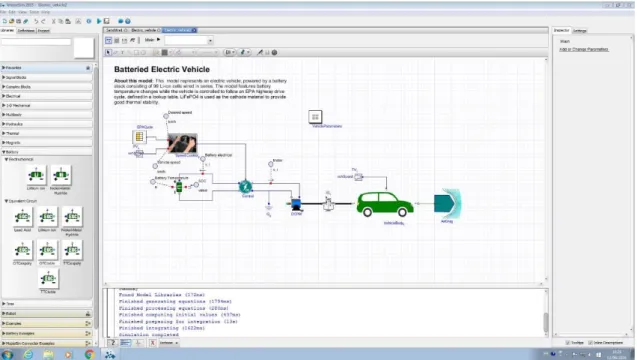
(13) Figure 1.3.- Schematic diagram for the DP model [6] This model allow to refine the description of polarisation characteristics of the battery and simulate the concentration polarisation and the electrochemical polarisation separately, which leads to an improved simulation at the moments of end of charge or discharge compared to the Thevenin model. The DP model is composed of three parts [6]:  . . The open-circuit voltage (Uoc), which is reproduced by a voltage source. Internal resistances such as the ohmic resistance R0 and the polarisation resistances, which include Rpa to represent the effective resistance characterising electrochemical polarisation and Rpc to represent the effective resistance characterising concentration polarisation. The effective capacitances like Cpa and Cpc, which are used to describe the electrochemical polarization and the concentration polarization separately and to characterise the transient response during transfer of power to/from the battery, more concretely the network Rpa and Cpa captures the short transients (STC) and the network Rpc and Cpc captures the long ones (LTC) [5].. Upa and Upc are the voltages across Cpa and Cpc respectively. Ipa and Ipc are the outflow currents of Cpa and Cpc respectively. The equations that describes the electrical behaviour of this circuit will be expressed in the section 2.1.. 1.6 MAPLESIM ENVIRONMENT The most part of this work has been developed thanks to the modelling, simulation and analysis tool MapleSim, which has, among others, a specific library for the batteries. It provided us with a wide range of different batteries models. This together with the different tools to create custom components has allow us to suit our modelling and simulation needs, and therefore fulfil the goals of this study. The integration of MapleSim and Maple offers more freedom in order to develop your models. Thanks to its flexibility, you are no longer restricted to built-in components or analyse. With its complete programming and analysis environment, it is possible to. 12.

(14) run simulations, customise analyses or script entirely new ones, perform optimisations, develop advanced symbolic control laws and investigate models in ways that are not possible with other tools [7]. It also allows to build component diagrams that represent physical systems in a graphical form, which is of great help for many engineers that do not find many existing simulation tools intuitive for physical modelling. Using both symbolic and numeric approaches, MapleSim automatically generates model equations from a component diagram and runs high-fidelity simulations [8]. After automatically generating these equations, MapleSim tries to simplify them with symbolic techniques that include index reduction, differential elimination, separation of independent systems, and elimination of redundant systems. The two main benefits of symbolic simplification are the following [8]: . By symbolically resolving algebraic loops and through reducing the complexity of DAEs, symbolic simplification makes many problems, which previously were intractable, numerically solvable.. . The simplified equations are provided to the numerical solvers in a computationally efficient form. This reduces the total simulation time, in some cases, by many orders of magnitude.. Computational efficiency is particularly important for studies that requires hardware-in-the-loop (HIL) simulation, such as the implementation of a batteries in the electric vehicle, because it allows to develop higher fidelity models while the real-time performance remains accurate.. Figure 1.4- Screenshot of MapleSim, showing all the different possibilities concerning battery simulation. 13.

(15) In Figure 1.4, we can see the appearance of MapleSim software. On the left-hand side of the screenshot, it is shown the two different approaches of battery modelling (electrochemical and EEC) that it allows, and some batteries of different nature that are already implemented in the software. As it was stated previously, during the development of this study the electrochemical and EEC models of the Lithium-ion battery were used, as well as the EEC model of the Lead-Acid battery, due to the fact that MapleSim does not include the electrochemical model of the latter.. 14.

(16) 2 MODELLING OF A LITHIUM-ION BATTERY Firstly, we started with the comparison between the two kinds of models that MapleSim allow us to use in order to describe the performance of a Lithium-ion battery. These models are the electrochemical model and the electrical equivalent circuit (EEC) model, also known as equivalent circuit models (ECM), which has been introduced in the section 1.5. So as to accomplish this task, we took the electrochemical model that MapleSim included in its battery library as a reference and we tried to obtain the same output with the electrical equivalent circuit (EEC) model. The equation that describe the behaviour of the EEC model in MapleSim is the following:. 𝑉𝑏𝑎𝑡𝑡 = 𝑁𝑐𝑒𝑙𝑙 ∙ (𝑉𝑜𝑐 − 𝑉𝑅𝑖𝑛𝑡 − 𝑉𝑅𝐶1 − 𝑉𝑅𝐶2 − ⋯ − 𝑉𝑅𝐶𝑛 ). ( 2.1 ). Where Vbatt is the terminal voltage, Ncell is the number of cells number of cells in series that compose the stack, in our study we considered a Lithium-ion battery with one cell (Ncell = 1) for almost every simulations, except in section 4.5. Voc corresponds to the open circuit voltage, VRint is the voltage drop across the internal resistance (Rint) and VRCn is the voltage drop across the n-th RC network. In this case, as we have established in section 1.5.3, we considered an electrical circuit with two RC networks, therefore its terminal voltage would be characterised by the equation ( 2.2 ):. 𝑉𝑏𝑎𝑡𝑡 = 𝑁𝑐𝑒𝑙𝑙 ∙ (𝑉𝑜𝑐 − 𝑉𝑅𝑖𝑛𝑡 − 𝑉𝑅𝐶1 − 𝑉𝑅𝐶2 ). ( 2.2 ). The layout of our model is presented in Figure 2.1. Each subsystem contains the electrochemical model (the one on the right) or the electrical equivalent circuit model (the left one). The content of each subsystem is the same excepting the battery model used. Figure 2.2 shows the EEC model subsystem.. Figure 2.1.- Layout of the model developed in MapleSim. 15.

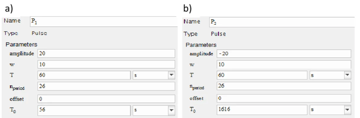
(17) Figure 2.2.- Content of the EEC model subsystem. Each source (P1 and P2) was configured to work in different periods of time. In order to achieve this, the configuration of the sources is shown in Figure 2.3. As a result, the input current obtained consist of a pulse train which firstly discharge the battery and then charge it, as depicted in Figure 2.4.. a). b). Figure 2.3.- Configuration of the source that: a) discharge the batteries; b) charge the batteries. Figure 2.4.- Input current: pulse train with an amplitude of -20 A, T=60 sec. and a width of 10% of the period During the 90% of the period the value of the current is 0 A and the remaining 10% the current is ±20A depending if we are in the discharging or charging period. Using. 16.

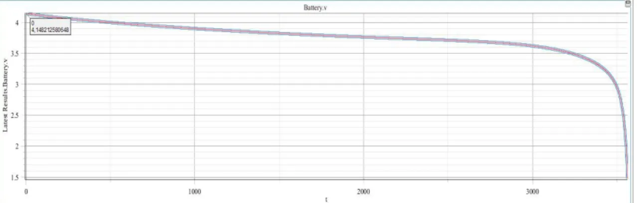
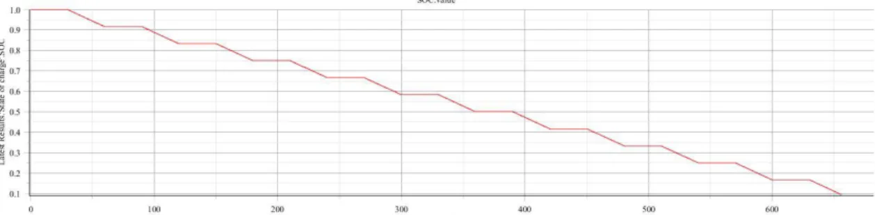
(18) this current as the input of our system, we obtain a comparison between the outputs of both models, electrochemical and EEC models, depicted in Figure 2.5 and Figure 2.6.. Figure 2.5.- Output: Terminal voltage of the electrochemical model (green) and the EEC model (red). Figure 2.6.- Output: State of Charge of the electrochemical model (green) and the EEC model (red) It can be seen that the results obtained from both models are very similar. Nevertheless, there is an estrange behaviour in the electrochemical one. For instance, concerning the Figure 2.6, when we study the state of charge of the battery, it is of the utmost importance to bear in mind that it depends on the current and the temperature. Therefore, if the input current is equal to zero the value of the state of charge must remain constant because these models were configured as isothermals, which means that the temperature remains constant during all the simulation. However, we can verify that the state of charge of the electrochemical model does not follow this behaviour. On the other hand, in Figure 2.5 it is represented the terminal voltage of both models. Here, the EEC model output is also more similar to the terminal voltage of a real battery, due to the fact that in the electrochemical model, when the current is zero the value of this output increase very abruptly and decrease a little bit later in the discharging period and vice versa when charging. Whereas for EEC model, we can clearly distinguish the contribution of the different components of the electrical circuit (Figure 1.3), which allow us to track the transients of the battery. When the input current becomes zero, firstly, there is a sudden increase of the output voltage due to the internal resistance, then the voltage keeps increasing but in a slower rate due to the parallel RC. 17.

(19) networks, describing the transient response. When charging it would be the other way round, firstly there is a sudden drop due to the internal resistance and then a moderate decrease due to the RC networks. In order to make sure that the EEC model tracks better the battery behaviour we carried out another simulation with both models, but in this case the input current would be a constant current (Figure 2.7).. Figure 2.7.- Input current: Constant current with an amplitude of +/-5 A. Figure 2.8.- Output: Terminal voltage of the electrochemical model (green) and the EEC model (red). Figure 2.9.- Output: State of Charge of the electrochemical model (green) and the EEC model (red) The behaviour of both models is almost the same for this step input with an amplitude of 5A when discharging and -5A when charging. Thus, taking everything into. 18.

(20) account we chose the EEC one as the reference battery model to carry out our study, as we verified that it was the one that describe the battery behaviour with the highest fidelity.. 2.1 IMPLEMENTATION OF THE BATTERY MODEL IN MATLAB ENVIRONMENT Once the EEC model was chosen as the reference model from which our study could be developed, we wanted to make sure that the parameters we were going to use in Matlab would allow us to have an accurate representation of the performance our battery model. The parameters used in Matlab were obtained from the EEC model that it was modelled in MapleSim. The value of each parameter depends on SOC, following the form of the equation ( 2.3 ). Where the variable “parameter” refers to the internal resistance (R0) or any of the components of the RC networks (R1, C1, R2 or C2). General form: 𝑝𝑎𝑟𝑎𝑚𝑒𝑡𝑒𝑟 = 𝑘1 ∙ 𝑒 𝑘2 ∙𝑆𝑂𝐶 + 𝑘3. ( 2.3 ). Particularised for each parameter: 𝑅0,𝑘 = 0,11 ∙ 𝑒 −50∙𝑆𝑂𝐶𝑘 + 0,0075 𝑅1,𝑘 = 0,05 ∙ 𝑒 −29∙𝑆𝑂𝐶𝑘 + 0,0074 𝑅1,𝑘 ∙ 𝐶1,𝑘 = 3,5 ∙ 𝑒 −10∙𝑆𝑂𝐶𝑘 + 10,5 𝑅2,𝑘 = 1 ∙ 𝑒 −150∙𝑆𝑂𝐶𝑘 + 0,008 𝑅2,𝑘 ∙ 𝐶2,𝑘 = −500 ∙ 𝑒 −20∙𝑆𝑂𝐶𝑘 + 710 The open circuit voltage (Voc) is also obtained from MapleSim and follows the same form of ( 2.3 ): 𝑉𝑂𝐶 𝑘 = 0,1958 ∗ 𝑒 1,332∙𝑆𝑂𝐶𝑘 + 3,429703601. ( 2.4 ). So as to implement this model in Matlab environment it was necessary to create a linear state-space model defined by this equations:. 19. 𝑥̇ = 𝐴𝑥 + 𝐵𝑢 + 𝑤. ( 2.5 ). 𝑦 = 𝐶𝑥 + 𝐷𝑢 + 𝐻𝑣. ( 2.6 ).

(21) We needed to rewrite the equations that described the electrical behaviour of the battery model into the matrix form, which fitted with the state-space formulation. This EEC model was based on the Dual Polarised circuit introduced in section 1.5.3. Our particular model is represented in Figure 2.10.. Figure 2.10.- Electrical equivalent circuit Model of the Battery. The controllable source represents the open circuit voltage (Voc). The function of the rest of the components has been detailed in section 1.5.3. The electrical behaviour of the previous circuit could be described by the following system of equations:. 𝑉1 𝐼𝑏𝑎𝑡𝑡 + 𝑅1 (𝑆) ∙ 𝐶1 (𝑆) 𝐶1 (𝑆) 𝑉2 𝐼𝑏𝑎𝑡𝑡 𝑉̇2 = − + 𝑅2 (𝑆) ∙ 𝐶2 (𝑆) 𝐶2 (𝑆) (𝑆, {𝑉𝑡𝑒𝑟𝑚 𝐼) = 𝑉𝑜𝑐 (𝑆) − 𝑉1 − 𝑉2 − 𝑅0 ∙ 𝐼𝑏𝑎𝑡𝑡 𝑉1̇ = −. ( 2.7 ). Bearing in mind that we were in a simulation environment, we chose the Coulomb counting method ( 2.8 ) in order to keep track of the SOC of our model implemented in Matlab as it assures 100% accuracy for ideal batteries working in this environment [5]:. 𝑆(𝐼) = 𝑆𝑖𝑛𝑖𝑡 +. 𝑡 1 ∙ ∫ 𝐼𝑏𝑎𝑡𝑡 (𝑡) 𝑑𝑡 𝐶𝑢𝑠𝑒 ∙ 3600 0. ( 2.8 ). Where Sinit represents the SOC at the initial time t0, Ibatt (t) the current traversing the battery in Amperes (assumed to be positive when discharging and negative when charging) and Cuse is the available usable capacity of the battery in Ampere-hour, which changes with the service life (in our particular case Cuse = 1Ah and it will remain constant during most of the simulations of this study, except for the simulations concerning the state of health of the battery). However, if we take into consideration the losses that. 20.

(22) occur while charging and discharging and also during storing periods, the equation ( 2.8 ) must be slightly modified [9]:. 𝑆(𝐼) = 𝑆𝑖𝑛𝑖𝑡 [1 −. 𝑡 𝜎 ɳ (𝑡 − 𝑡0 )] + ∙ ∫ 𝐼𝑏𝑎𝑡𝑡 (𝑡) 𝑑𝑡 24 𝐶𝑢𝑠𝑒 ∙ 3600 0. ( 2.9 ). Where σ is the self-discharge rate, which depends on the accumulated charge and the battery state of health (SOH). A value of 0,2% per day is recommended for this parameter; ɳ is the coulombic efficiency1, which it is assumed to be one for discharging and less than or close to one when charging, in order to reflect the fact that only a fraction of the input energy is restored. It depends on the technology used for the battery and other variables such as the temperature, the charging/discharging current, the state of charge (SOC) and the state of health (SOH). In our particular case, as we work in the ideal conditions that characterised the simulation environment, it is assumed to be constant and equal to one in both charging and discharging process, and the self-discharge rate is going to be fixed to 0% for the same reason [10]. In order to adapt this equations to the state-space formulation we defined the following matrix based on the equations ( 2.7 ) and ( 2.8 ):. 𝐴=. 1 − 𝑅1 ∙ 𝐶1 0 [. 0. 0 −. 1 𝑅2 ∙ 𝐶2 0. 1 𝐶1 0 1 𝜕𝑉𝑂𝐶 ; 𝐵= ; 𝐶 = [−1 −1 ]; 𝐶2 0 𝜕𝑆𝑂𝐶 1 − 0] [ 𝐶𝑢𝑠𝑒 ∙ 3600]. 𝑉1 𝐷 = [−𝑅0 ] ; 𝐻 = [1] ; 𝑥 = [ 𝑉2 ] ; 𝑢 = [𝐼𝑏𝑎𝑡𝑡 ] ; 𝑦 = [𝑉𝑡𝑒𝑟𝑚 ] 𝑆𝑂𝐶. ( 2.10 ). At first, we started implementing a linear model of the reference battery. Therefore, all the nonlinear expressions were linearized. Concerning the circuit parameters defined in ( 2.3 ), we supposed that their value remained constant and equal to their initial value when the battery was fully charged (SOC=1) during all the simulation. Whereas the expression of the open circuit voltage (Voc) was linearized using the curve fitting tool from Matlab and an excel file with data from the battery model in MapleSim so as to fit these data with a linear curve. The linearized expression of the Voc is defined as follows: 𝑉𝑂𝐶 𝑘 = 0.5552 ∗ 𝑆𝑂𝐶𝑘 + 3,525 1. ( 2.11 ). Coulombic efficiency: The ratio of the number of charges that enter to the battery during charging and those that can be extracted from the battery during discharging.. 21.

(23) Once our model in Matlab was defined, we proceeded to verify if this system was able to reproduce the same behaviour as that of our battery model in MapleSim. In order to carry out this verification we introduced the same excitations for the two systems and compared their outputs. For instance, using a constant current of 1A as the input, we obtain the following outputs:. Figure 2.11.- Battery terminal voltage response in Matlab using a constant current of 1A. Figure 2.12.- Battery Voltage response in MapleSim using a constant current of 1A. Although at a first glace it may seem that these two systems do not have any similarities between them, we have to take into account that when we transform a model into a linear state-space model we are linearizing the model, so the system will lose all the properties related to its nonlinearities. Therefore, we have to analyse the area where the model has a linear behaviour. If we do so, we are going to find that both systems have almost the same behaviour in their flatter part.. 22.

(24) Figure 2.13.- State of charge (SOC) response in Matlab using a constant current of 1A. Figure 2.14.- State of charge (SOC) response in MapleSim using a constant current of 1A It can be seen that the battery state of charge in both cases decrease at the same rate. In order to make sure that we could continue working with this model in Matlab, we introduced a new input current to the system, consisting of a square-wave pulse train with an amplitude of 10A and a period of 60 seconds during 679 seconds until the 10% of the SOC was reached, as it is shown in Figure 2.15.. Figure 2.15.- Input current: train of square-wave pulses with an amplitude of 10A and T=60 sec. 23.

(25) Using this current as the battery model input, we obtain the following responses, in both Matlab and MapleSim. We can verify that we achieve a great accuracy in the estimation, being the linearization of the system in Matlab the reason of the small differences that exist between both models.. Figure 2.16.- Battery Terminal Voltage response in Matlab. Figure 2.17.- Battery Terminal Voltage response in MapleSim. Figure 2.18.- State of charge (SOC) response in Matlab using an input current that consist of train of square-wave pulses. 24.

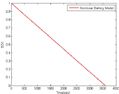
(26) Figure 2.19.- State of charge (SOC) response in MapleSim using an input current that consist of train of square-wave pulses. From the previous graphics it is visible that this model is highly accurate if we work with a battery that has a linear behaviour. However, due to the inherent nonlinear nature of the battery behaviour, the nonlinear model was also implemented in Matlab, as it accounts for the nonlinearities. This model was developed considering that R0, R1, C1, R2, C2 and Voc depend nonlinearly on SOC, as it was defined in equations ( 2.3 ) and ( 2.4 ).. As we wanted to prove that this model accounts for the nonlinearities of the system, we used the same constant current as that which has been previously used to show that the linear system gives a good estimation of the terminal voltage only in the flatter area of the curve. Making a comparison between the outputs depicted in Figure 2.20 and Figure 2.12, we can confirm that with this model we also keep track of the nonlinearities of the battery model to some extent.. Figure 2.20.- Battery terminal voltage of the nonlinear system implemented in Matlab using a constant current of 1A as the input of the system. 25.

(27) Figure 2.21.- SOC of the nonlinear system implemented in Matlab using a constant current of 1A as the input of the system. All things considered, we decided to start the simulations in Matlab with the linear system in order to develop the Simple Kalman Filter (SKF), due to the fact that it has been proved that it operates better when it works with linear systems. Later on, we would change to the nonlinear system so as to implement the Extended Kalman Filter, as we will see in chapter 3.. 26.

(28) 3 STATE OF CHARGE ESTIMATION ALGORITHM 3.1 STATE OF THE ART State of charge estimation of commercial batteries can be done by many different methods in electrical chemistry laboratory like coulometric titration technique [3]. But this estimation is quite challenging without destruction of the battery or interruption of the battery power supply, especially the applications which require online estimations. Currently there has been intensive study on SOC estimation algorithm. Below a short review of some of them is presented [3]:. . Discharge test method This test could precisely find the remaining charge of the battery and then the SOC under controlled conditions, i.e., specified discharge current and ambient temperature. Its major drawback is that it is a time-consuming method and after the test the battery have no power, hence this method is not useful for the online applications of the batteries, reducing its utility to the laboratory environment only.. . Coulomb counting (Ampere-Hour integral) method This is the most simple and general method to obtain the battery SOC. It is characterised by the equation ( 2.8 ) that has been defined before. If the initial estimation of SOC is relatively precise, the results of the Coulomb counting method are quite satisfactory. Nevertheless, it has several disadvantages: i) It cannot get the precise initial SOC automatically, so it is highly important to have an accurate initial estimation of SOC in order to obtain a precise SOC estimation. ii) The Coulombic efficiency (ɳ) can be influenced by the operation state of the battery, such as SOC, temperature, etc., which are difficult to measure and then produce cumulative effects on SOC error. iii) Its dependence on the precision of the current sensor that will result in cumulative effects which will influence on the precision of SOC. Therefore, the Coulomb counting method alone cannot meet the requirement of SOC precision.. 27.

(29) . Open circuit voltage (OCV) method The one to one correlation between OCV and SOC make this method an effective one to estimate SOC of Lithium-ion batteries, because it allows us to be sure that when the battery has reached balance after adequate resting, the OCV corresponds to 100% of the SOC. This method give us a high precision SOC estimation but, on the other hand, the relaxation period requires a lot of time until the batteries reach balance. It usually take some time for them to recover from an operating state to a balanced state, this duration depends on the SOC and temperature of the battery among others. Thus, this method, if used alone, is suitable only for applications where the device is left idle, for instance, for the electric vehicles (EVs) case, this method will be useful only if they are parking rather than driving. Moreover, careful consideration and research are needed as the OCV of some kinds of batteries depends on the charge/discharge process. For instance, the charge and discharge open circuit voltage of Lithium-ion phosphate (LFP) batteries experience the hysteresis phenomena as indicated in Figure 3.1 [11]:. Figure 3.1.- Flat OCV-SOC curve for the LFP cell (20°C) after a 3-hour rest period [11]. Considering the hysteresis phenomena of LFP battery, it has been shown that the hysteresis is correlated with the relaxation time, with the level of hysteresis decreasing as the rest period increases. This phenomenon is depicted in the Figure 3.2 where the voltage was plotted with respect to SOC for different relaxation periods.. 28.

(30) Figure 3.2.- Hysteresis decreases with the increase of the rest time in the multiple-step test conducted on the LFP cell at 20°C [11] . Battery model-based SOC estimation method The OCV method needs enough time resting to complete the relaxation period accurately, hence, it is not useful for online applications when the device is working, for example, while the electric vehicle is driving. In such cases, the construction of battery model in conjunction with OCV method is necessary in order to online estimate the OCV during operation. The most commonly used battery models include electrical equivalent circuit (EEC) model and electrochemical model, which have been introduced in section 1.5. Remind that the terminal voltage of the EEC model derived from the Thevenin Model, could be expressed as:. 𝑈𝐿 = 𝑈𝑂𝐶 − 𝑈𝑇ℎ − 𝐼𝐿 𝑅0. ( 3.1 ). Where UL is the battery terminal voltage, the product 𝐼𝐿 𝑅0 represent the voltage drop caused by the ohmic resistance, UOC the battery OCV and UTh is the voltage drop across the parallel RC networks. So it is easy to found the value of the OCV if the battery model parameters are known. The direct relation between OCV and SOC allow us to easily found the SOC by using an OCV-SOC look-up table. For this method, the precision and complexity of battery model are very important. We have seen in the previous chapter that the desire to achieve a good compromise between accuracy and computation time, lead us to choose the EEC model composed of two RC networks among the wide variety of different battery models thanks to its accurate performance (with a mean error of 1.4%). 29.

(31) despite its low computational intensity. Whereas the electrochemical model, due to its high complexity, usually is only used for the battery performance analysis and battery design. . Neural network model method It is based on the use of nonlinear mapping characteristics of the neural network so as to estimate the SOC. When building a model, the neural network method does not have to take into account specific details of a battery as it is suitable for all kinds of batteries. Nevertheless, it needs a great number of training sample data to train the method. Moreover, this method requires a lot of computations, which makes necessary to have powerful processing chips.. . Fuzzy logic method It is based on the simulation of the thinking of human beings by using the fuzzy logic on the basis of a great number of test curves, experience and reliable fuzzy logical theories. It eventually could be used to predict the SOC of the battery but it requires a deep understanding of the batteries themselves and a large number of computations.. . Integrated algorithm based on the two or more of the above methods Currently there are several integrated methods such as: o Simple correction integrated algorithm: It includes Ampere-Hour integrated algorithm with correction by open circuit voltage, Ampere-Hour integral method with SOC calibration after charging and so on. For batteries in pure electric vehicles: .  . The working conditions are simple: when the vehicles are moving, their batteries are mainly in a discharge state, and when the batteries are being charged in a charging station, the batteries are in a charge state. Moreover the hysteresis of the open circuit voltage is easy to estimate. Thanks to the large capacities of the batteries the errors of the Ampere-Hour integral are relatively low. The possibility to be fully charge is great. All the above things considered, we can affirm that the Ampere-Hour method with initial SOC correction according to the open circuit voltage and SOC calibration after full charging could meet the precision requirement of SOC. 30.

(32) estimation of pure electric vehicles. However for batteries in hybrid electric vehicles (HEV) this method is unable to meet the requirements due to the following reasons: .  . The complexity of the working conditions because when the vehicles are moving, the current is both charged and discharged so as to keep the battery SOC in a narrow range. Due to the small capacities of the batteries the errors of the AmpereHour integral are high. There is no opportunity of full charging when the vehicles ae parked, except for maintenance.. Therefore, for the HEB other integrated methods are needed. o Weighted fusion algorithm This algorithm is to add up the SOC estimated through different methods in accordance with certain weights to obtain SOC. Figure 3.3 shows the operation of this algorithm:. Figure 3.3.- weighted fusion algorithm from [3] o Kalman filtering Due to the impossibility of direct SOC measurement, two methods of SOC estimation are integrated as a dynamic system, in which SOC is regarded as an internal state of the system and is analysed. Furthermore, in order to take into consideration the nonlinearities of the battery, the Extended Kalman Filter (EKF) method is usually adopted. Generally, researches are conducted through systems formed by the Coulomb counting method and other battery models. In [12] it was pointed out that the meaning of EKF as a state observer lies in: when the SOC is estimated using the Coulomb counting method, the. 31.

(33) voltage of the capacitor is estimated and then the estimation values of the cell terminal voltage are obtained to act as a basis for correcting SOC; meanwhile noises and errors are taken into account, filtering gains of each step is determined in order to minimise the a posteriori error covariance, and eventually the optimal estimation of SOC is also obtained. In this way, with the combination of the Coulomb counting method and the model-based SOC estimation (Kalman Filter), which overcomes the shortcoming of cumulative errors that characterised the former, we can achieve a SOC closed-loop estimation. Moreover, since the measurement and process noise are taken into consideration, the algorithm has a strong inhibiting effect on noises, what makes it a robust method. The Kalman filtering method used for SOC estimation relies on a reasonable battery equivalent model and a group of state equations. Therefore, as this method is highly dependent on the battery model, an accurate battery model is needed to be established so as to obtain a reliable SOC estimation. The model should not be too complex in order to save computations, but it should not be too simple either, to achieve an accurate resemblance with the battery that we are studying. Finally it is important to highlight that if the selection of the filtering gain is undesirable, the state will disperse. o Sliding mode observer So as to overcome the limitations of the Kalman filter method, the slip mode observer technology is used, which possesses strong robustness against the uncertainty of the model parameters and disturbance. The problem is that it is complicated to implement. Taking everything into account, we determined that the Kalman Filter algorithm was the most suitable method to estimate the SOC of our battery due to its good compromise between accuracy and computational intensity.. 3.2 INTRODUCTION TO DISCRETE SIMPLE KALMAN FILTER Kalman filter (KF) is a well-known estimation theory introduced in 1960. The filter tries to estimate the systems state variables by providing a recursive solution through a linear optimal filtering [13]. As it was explained in section 3.1, this particular model-based state-estimation technique is proposed to estimate the state of a battery cell that are normally difficult or expensive to measure. It is widely used due to its interesting characteristics. Among other things, it can optimally (searching the minimum variance) estimate the states. 32.

(34) affected by a broadband noise contained within the system bandwidth, that cannot otherwise be filtered out using classical techniques [14]. We were based on the state space formulation defined in ( 2.5 ) and ( 2.6 ) for developing the Kalman Filter. However, in order to use this algorithm, it is necessary to consider that the battery model, of which we are trying to estimate the state vector, xk, which includes the SOC among others, is governed by the discrete linear equation ( 3.2 ), whose output vector, yk, is defined in ( 3.3 ).. 𝑥𝑘 = 𝐴𝑥𝑘−1 + 𝐵𝑢𝑘−1 + 𝑤𝑘−1. ( 3.2 ). 𝑦𝑘 = 𝐶𝑥𝑘 + 𝐷𝑢𝑘 + 𝑣𝑘. ( 3.3 ). Equation ( 3.2 ) is known as the state or process equation, where A ϵ Rnxn is the matrix that describes the system dynamics and relates the state at the previous time step k-1 to the current time step k when the control input u k-1 is equal to zero, and B ϵ Rnxp relates the control input uk-1 to the state xk. Whereas the equation ( 3.3 ) is called the output or measurement equation. The transformation matrix C ϵ Rmxn and the feedforward matrix D ϵ Rmxp relate the output yk to the state xk and the input uk, respectively. The process noise, wk, and the measurement noise, vk, are assumed to be random variables, independent of each other, white and with normal probability distributions [15]:. 𝑝(𝑤)~𝑁(0, 𝑄). ( 3.4 ). 𝑝(𝑣)~𝑁(0, 𝑅). ( 3.5 ). In practice, the process noise covariance Q and the measurement noise covariance are supposed to be variable throughout time, however in this study we are going to consider them to be constants for all the simulations.. 33.

(35) 3.2.1 STATE OF CHARGE ESTIMATION BASED ON SIMPLE KALMAN FILTER ALGORITHM FOR LITHIUM-ION BATTERIES Once it was verified that the battery model implemented in Matlab gave an accurate description of the MapleSim system behaviour, and the system of equations that governed our battery model was discretised, we continued trying to implement the Simple Kalman filter (SKF) so as to estimate the state vector xk, which is the same as the vector “x” defined in ( 2.10 ) but discretised. The discrete SKF algorithm is defined as follows: First of all the Kalman Filter must be initialised:. 𝑥̂𝑘−1 = 𝐸(𝑥0 ) ; 𝑃𝑘−1 = 𝐸[(𝑥0 − 𝑥̂0 )(𝑥0 − 𝑥̂0 )𝑇 ]. ( 3.6 ). The state vector initialisation is obtained from the expected value that we would think the real state vector would have. The error covariance matrix P is initialised by obtaining the covariance matrix as defined in ( 3.6 ). Normally, these quantities are not precisely known, but this is not a problem due to the robustness to poor initialisation that characterises the Kaman Filter, and it will quickly converge to the true value as it runs [16].. Time update: 1. A priori state estimate update: 𝑥̂𝑘− = 𝐴𝑥̂𝑘−1 + 𝐵𝑢𝑘−1. ( 3.7 ). 2. Error covariance time update: 𝑃𝑘− = 𝐴𝑃𝑘−1 𝐴𝑇 + 𝑄. ( 3.8 ). Measurement update: 3. Kalman gain matrix 𝐾𝑘 = 𝑃𝑘− 𝐶 𝑇 (𝐶𝑃𝑘− 𝐶 𝑇 + 𝑅)−1. ( 3.9 ). 4. Measurement residual 𝑦̃𝑘 = 𝑦𝑘 − (𝐶𝑥̂𝑘− + 𝐷𝑢𝑘 ). ( 3.10 ). 5. A posteriori state estimate update 𝑥̂𝑘 = 𝑥̂𝑘− + 𝐾𝑘 𝑦̃𝑘. 34. ( 3.11 ).

(36) 6. Estimated output 𝑦̂𝑘 = 𝐶𝑥̂𝑘 + 𝐷𝑢𝑘. ( 3.12 ). 7. Error covariance measurement update 𝑃𝑘 = (𝐼 − 𝐾𝑘 ∙ 𝐶) ∙ 𝑃𝑘−. ( 3.13 ). 8. Repeat steps one to seven until the simulation ends The state of charge is tracked by using the expression defined in ( 2.8 ). Moreover, as we were working with the Simple Kalman Filter, it was necessary to use the linear expression of the open circuit voltage (Voc), which was expressed in equation ( 2.11 ). Finally, in order to implement this algorithm using ( 3.2 ), the matrices defined in ( 2.10 ) must be discretised:. 𝐴=[. −𝑇𝑠 𝑅 1,𝑘 𝑒 ∙𝐶1,𝑘. 0 0. 𝑅1,𝑘 ∙ (1 − 0. 0. 0. 0 1. −𝑇𝑠 𝑒 𝑅2,𝑘∙𝐶2,𝑘. −𝑇𝑠. ] ; 𝐵 = 𝑅2,𝑘 ∙ (1 − 𝑒 𝑅2,𝑘∙𝐶2,𝑘 ) ; [. 𝐶 = [−1 −1. −𝑇𝑠 𝑅 1,𝑘 𝑒 ∙𝐶1,𝑘 ). −𝑇𝑠 𝐶𝑢𝑠𝑒,𝑘 ∙ 3600. ]. 𝛿𝑉𝑂𝐶,𝑘 ] ; 𝐷 = [−𝑅0,𝑘 ] ; 𝐻 = [1] 𝛿𝑆𝑂𝐶𝑘. ( 3.14 ). And the output equation ( 3.3 ) is expressed by the following equation:. 𝑦𝑣𝑘 = 𝑉𝑡𝑒𝑟𝑚𝑣,𝑘 = 𝑉𝑜𝑐,𝑘 (𝑆𝑂𝐶𝑘 ) − 𝑉𝐶1,𝑘 − 𝑉𝐶2,𝑘 − 𝐼𝑏𝑎𝑡𝑡,𝑘 ∙ 𝑅𝑖𝑛𝑡,𝑘 + 𝑣𝑘 ( 3.15 ) Implementing this algorithm in Matlab with the parameters defined before, (2.3), we obtained the following response, which was compared to the response of the discrete linear system defined in ( 3.3 ) and ( 3.15 ):. Where:. 10−6 𝑄=[ 0 0. 0 10−6 0. 0 0 ] 10−6. 𝑎𝑛𝑑. 𝑅 = 1.5. 0.1 0.0009 And the algorithm initialization: 𝑥̂ = [0.5] ; 𝑃 = [ 0.0047 0.9 −0.0009. 35. 0.0047 0.0233 −0.0047. −0.0009 −0.0047] 0.0009.

(37) Figure 3.4.- Comparison between linear system and Simple Kalman Filter SOC estimation for an input which consists of a constant current of 1A. Figure 3.5.- Comparison between linear system and Simple Kalman Filter terminal voltage estimation for an input which consists of a constant current of 1A. Figure 3.6.- Comparison between linear system and Simple Kalman Filter voltage drop estimation in the first RC network for an input which consists of a constant current of 1A. 36.

(38) Figure 3.7.- Comparison between linear system and Simple Kalman Filter voltage drop estimation in the second RC network for an input which consists of a constant current of 1A. It is visible from the previous graphics that the Simple Kalman Filter makes a good estimation when we are working with linear systems despite the strong measurement noise (Figure 3.5). In a simulation environment, as we are in ideal conditions, the Coulomb counting method is supposed to give the right estimation of the SOC as we do not have errors in the measurements. The input was changed to a square wave pulse train with an amplitude of 10A, conserving the previous initialisations. The results obtained are the following:. Figure 3.8.- Comparison between linear system and Simple Kalman Filter SOC estimation for an input which consists of a square wave pulse train with an amplitude of 10A. 37.

(39) Figure 3.9.- Comparison between linear system and Simple Kalman Filter terminal voltage estimation for an input which consists of a square wave pulse train with an amplitude of 10A. Figure 3.10.- Comparison between linear system and Simple Kalman Filter voltage drop estimation in the first RC network for an input which consists of a square wave pulse train with an amplitude of 10 A. Figure 3.11.- Comparison between linear system and Simple Kalman Filter voltage drop estimation in the second RC network for an input which consists of a square wave pulse train with an amplitude of 10. 38.

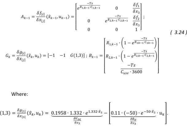
(40) We can observe that in this case, as the input current experiences abrupt changes, the SOC estimation is not as good as for the constant current. The SKF struggles due to the non-linear behaviour of the battery terminal voltage, Vterm. This is to be expected as the algorithm is trying to minimise the error between non-linear process (Vterm) and a linear equation by varying SOC away from its true value. At this point, we wanted to improve this estimation, thus we proceeded with the implementation of the Extended Kalman Filter, which is able to keep track of the nonlinearities of the system. In order to do that we implemented also the nonlinear battery model, which was introduced in section 2.1. The procedure followed will be seen in the next section.. 3.3 EXTENDED KALMAN FILTER As it was said previously, in reality Voc, R1, C1, R2 and C2 are nonlinearly dependant on SOC, therefore it is necessary to consider that our system (the battery model), whose state vector xk (which includes SOC) is the aim of our estimation, is governed by the discrete nonlinear difference stochastic equation ( 3.16 ) whose measurement vector yk is given by the equation ( 3.17 ). Where f(.,.) is a nonlinear state transition function and g(.,.) is a nonlinear measurement function.. 𝑥𝑘 = 𝑓(𝑥𝑘−1 , 𝑢𝑘−1 ) + 𝑤𝑘−1. ( 3.16 ). 𝑦𝑘 = 𝑔(𝑥𝑘 , 𝑢𝑘 ) + 𝑣𝑘. ( 3.17 ). As before, wk and vk are assumed to be mutually uncorrelated white Gaussian random processes, with zero mean and covariance matrices Q and R, ( 3.4 ) and ( 3.5 ), respectively. Now, at each time step f(xk-1,uk-1) and g(xk,uk) are linearised by a first-order Taylor-series expansion. We assume that f(.,.) and g(.,.) are differentiable at all operating points (xk,uk), as shown in ( 3.18 ) and ( 3.19 ). As we can deduce from these expressions, the matrices A and G (which replaces C) are now Jacobian matrices Ak-1 and Gk of partial derivatives with respect to x. 𝑓(𝑥𝑘−1 , 𝑢𝑘−1 ) ≈ 𝑓(𝑥̂𝑘−1 , 𝑢𝑘−1 ) +. 𝜕𝑓(𝑥𝑘−1 , 𝑢𝑘−1 ) | 𝜕𝑥 𝑘−1 𝑥 ⏟. (𝑥𝑘−1 − 𝑥̂𝑘−1 ). ̂𝑘−1 𝑘−1 =𝑥. ( 3.18 ). 𝑑𝑒𝑓𝑖𝑛𝑒𝑑 𝑎𝑠 𝐴𝑘−1. 𝑔(𝑥𝑘 , 𝑢𝑘 ) ≈ 𝑔(𝑥̂𝑘 , 𝑢𝑘 ) +. 𝜕𝑔(𝑥𝑘 , 𝑢𝑘 ) | 𝑥 ⏟ 𝜕𝑥𝑘. (𝑥𝑘 − 𝑥̂𝑘 ) ̂𝑘 𝑘 =𝑥. ( 3.19 ). 𝑑𝑒𝑓𝑖𝑛𝑒𝑑 𝑎𝑠 𝐺𝑘. If we combine the equations ( 3.16 ) and ( 3.17 ) with ( 3.18 ) and ( 3.19 ), and we transform them into the state space formulation defined in ( 2.5 ) and ( 2.6 ), we. 39.

(41) obtain the equations that describe the nonlinear system, where matrices A, B, G and D are now subscripted with k so as to highlight that they also vary with time. 𝑥𝑘 = 𝐴𝑘−1 ∙ 𝑥𝑘−1 + 𝐵𝑘−1 ∙ 𝑢𝑘−1 + 𝑤𝑘−1. ( 3.20 ). 𝑦𝑘 = 𝐺𝑘 ∙ 𝑥𝑘 + 𝐷𝑘 ∙ 𝑢𝑘 + 𝑣𝑘. ( 3.21 ). The EKF algorithm remains almost the same as that of the SKF (from ( 3.7 ) to (3.13 )), with only steps 1, 4 and 6 changing, as it is shown in Figure 3.12.. Figure 3.12.- Extended Kalman Filter algorithm. 3.3.1 STATE OF CHARGE ESTIMATION BASED ON EXTENDED KALMAN FILTER ALGORITHM FOR LITHIUM-ION BATTERIES Aiming to implement this algorithm in Matlab, we defined the nonlinear functions f(.,.) and g(.,.) as well as their respective matrices, A and G.. 𝑓(𝑥𝑘−1 , 𝑢𝑘−1 ) = 𝐴𝑘−1 ∙ 𝑥𝑘−1 + 𝐵𝑘−1 ∙ 𝑢𝑘−1. ( 3.22 ). 𝑔(𝑥𝑘 , 𝑢𝑘 ) = ⏟ 0,1958 ∗ 𝑒 1,332∙𝑥3,𝑘 + 3,429703601 − 𝑥1,𝑘 − 𝑥2,𝑘 𝑉𝑜𝑐 𝑑𝑒𝑓𝑖𝑛𝑒𝑑 𝑖𝑛 ( 2.4 ). − (0.11 ⏟ ∙ 𝑒 −50∙𝑥3,𝑘 + 0.0075) ∙ 𝑢𝑘 𝑅0 𝑑𝑒𝑓𝑖𝑛𝑒𝑑 𝑖𝑛 ( 2.3 ). 40. ( 3.23 ).

(42) −𝑇𝑠. 𝐴𝑘−1 =. 𝛿𝑓[𝑖] (𝑥̂ , 𝑢 ) = 𝛿𝑥[𝑗] 𝑘−1 𝑘−1. 𝑒 𝑅1,𝑘−1∙𝐶1,𝑘−1. 0. 0. 𝑒 𝑅2,𝑘−1∙𝐶2,𝑘−1. 0. 0. 𝛿𝑓1 𝛿𝑥3 𝛿𝑓2 ; 𝛿𝑥3 1 ]. −𝑇𝑠. [. 𝑅1,𝑘−1 ∙ (1 − 𝐺𝑘 =. 𝛿𝑔[𝑖] (𝑥̂ , 𝑢 ) = [−1 𝛿𝑥[𝑗] 𝑘 𝑘. −1. ( 3.24 ). −𝑇𝑠 𝑒 𝑅1𝑘−1∙𝐶1𝑘−1 ) −𝑇𝑠. 𝐺(1,3)] ; 𝐵𝑘−1 = 𝑅2,𝑘−1 ∙ (1 − 𝑒 𝑅2,𝑘−1∙𝐶2,𝑘−1 ) [. −𝑇𝑠 𝐶𝑢𝑠𝑒 ∙ 3600. ]. Where: 𝛿𝑔. [1] 𝐺(1,3) = 𝛿𝑥 (𝑥̂𝑘 , 𝑢𝑘 ) = ⏟ 0.1958 ∙ 1.332 ∙ 𝑒 1.332∙𝑥̂3 − [0.11 ⏟ ∙ (−50) ∙ 𝑒 −50∙𝑥̂3 ∙ 𝑢𝑘 ]. [3]. 𝜕𝑉𝑜𝑐 𝜕𝑥3. 𝜕𝑅𝑜 𝜕𝑥3. The matrix A defined in ( 3.24 ) was simplified due to some singularity problems experienced during the implementation of the algorithm in Matlab. Hence, we ended up using the expression of this matrix defined in ( 3.14 ), which had been employed for the Simple Kalman Filter too. The singularity problems were caused because the denominators of the terms. 𝛿𝑓1 𝛿𝑥3. 𝛿𝑓. and 𝛿𝑥2 reached such a small values that they became 3. infinite. Using a constant current of 1A as the input of our system we obtain the results depicted from Figure 3.13 to Figure 3.16. The matrices Q, R, as well as the initialisations of 𝑥̂ and P are the same as for the SKF.. Figure 3.13.- Comparison between nonlinear system (red) and Extended Kalman Filter (blue) SOC estimation for an input which consists of a constant current of 1A. 41.

(43) Figure 3.14.- Comparison between nonlinear system (red) and Extended Kalman Filter (blue) terminal voltage estimation for an input which consists of a constant current of 1A. Figure 3.15.- Comparison between nonlinear system (red) and Extended Kalman Filter (blue) voltage drop estimation in the first RC network for an input which consists of a constant current of 1A. Figure 3.16.- Comparison between nonlinear system (red) and Extended Kalman Filter (blue) voltage drop estimation in the second RC network for an input which consists of a constant current of 1A. 42.

(44) From these graphics we can affirm that, for this particular input current, this algorithm makes a good estimation. Despite the good estimation that the SKF also gave for the same input, if we compare the Figure 3.7 and Figure 3.16, which represent estimation of the voltage drop in the second RC network (V2) using the SKF and the EKF, respectively, we can state that we achieve a faster convergence to the true vale with the latter. Therefore, for this input the estimation with the EKF has improved. Keeping track of the errors, we obtain that the mean absolute error of the terminal voltage (Vterm) estimation is 0,0032V and the relative error of this estimation is 0,00078067. Concerning the SOC estimation for this particular input, the value of the mean absolute error is 0,007. This values can support what we have just declared in the previous paragraph. As SKF algorithm showed some problems of convergence with the input current which consists of a square wave pulse train of 10 A. We introduced the same input to the EKF in order to reaffirm that this algorithm provides better estimations. The initialisation matrices were the same as before.. Figure 3.17.- Comparison between nonlinear system (red) and Extended Kalman Filter (blue) SOC estimation for an input which consists of a square wave pulse train with an amplitude of 10A. Figure 3.18.- Comparison between nonlinear system (red) and Extended Kalman Filter (blue) terminal voltage estimation for an input which consists of a square wave pulse train with an amplitude of 10A. 43.

(45) Figure 3.19.- Comparison between nonlinear system (red) and Extended Kalman Filter (blue) voltage drop estimation in the first RC network for an input which consists of a square wave pulse train with an amplitude of 10A. Figure 3.20.- Comparison between nonlinear system (red) and Extended Kalman Filter (blue) voltage drop estimation in the second RC network for an input which consists of a square wave pulse train with an amplitude of 10A Keeping track of the errors, we obtain that the mean absolute error of the terminal voltage (Vterm) estimation is 0,014706 V and the relative error of this estimation is 0,0036. Concerning the SOC estimation for this particular input, the value of the mean absolute error is 0,00812. This values are a little bit higher than those for the previous input, but anyway, with this algorithm the estimations are better compared to that of the SKF by far. From the comparison between the SOC estimation obtained from the SKF algorithm (Figure 3.8) and that from the EKF algorithm ( Figure 3.17 ), we can deduce that the SOC estimation is highly improved using the EKF algorithm. Not only does it arrive to the true value but it converges very quickly. Comparing the estimation of the voltage drop in the second RC network (V2) it is also visible the important improvement achieved by the EKF.. 44.

(46) Finally, in order to make sure that this algorithm makes good estimations for a wide range of different inputs, we decided to introduce an input which consists of a constant current of 50 A. As our battery was not originally designed to support such a strong current, the estimation did not have to be as perfect as for the previous cases. However, we verified that, in spite of the strong current, the estimation was quite good with a mean absolute error of the terminal voltage (Vterm) of 0,1057V and a relative error of this estimation of 0,0316. Concerning battery SOC, it was estimated with a mean absolute error of 0,0168. These errors are really small bearing in mind that the battery is not conceived for this kinds of strong inputs. The results that could corroborate what it was stated in the previous paragraph are depicted from Figure 3.21 to Figure 3.24.. Figure 3.21.- Comparison between nonlinear system (red) and Extended Kalman Filter (blue) SOC estimation for an input which consists of a constant current of 50A. Figure 3.22.- Comparison between nonlinear system (red) and Extended Kalman Filter (blue) terminal voltage estimation for an input which consists of a constant current of 50A. 45.

(47) Figure 3.23.- Comparison between nonlinear system (red) and Extended Kalman Filter (blue) voltage drop estimation in the first RC network for an input which consists of a constant current of 50A. Figure 3.24.- Comparison between nonlinear system (red) and Extended Kalman Filter (blue) voltage drop estimation in the second RC network for an input which consists of a constant current of 50A. Finally, once we had confirmed that the EKF enhance all the estimations compared to the SKF, and in order to verify that the EKF algorithm also provided good estimations after several cycles of charge and discharge, we created a script in Matlab in which it was possible to define the number of cycles that our battery model and EKF would be subjected to. In this case, the number of cycles was fixed to five and the input current was the same square wave pulse train with an amplitude of 10 A and a period of 60 seconds that it was used in the simulations for the SKF and the EKF.. 46.

(48) Figure 3.25.- Profile of the input current: 5 complete cycles of discharge and charge consisting of a square pulse wave with an amplitude of +/- 10A and T=60 sec. Figure 3.26.- Comparison between nonlinear system (red) and Extended Kalman Filter (blue) SOC estimation for an input which consists of a square wave pulse train with an amplitude of 10A and T=60sec. Figure 3.27.- Figure 3.18.- Comparison between nonlinear system (red) and Extended Kalman Filter (blue) terminal voltage estimation for an input which consists of a square wave pulse train with an amplitude of 10A and T=60sec. 47.

(49) Figure 3.28.- Comparison between nonlinear system (red) and Extended Kalman Filter (blue) voltage drop estimation in the first RC network for an input which consists of a square wave pulse train with an amplitude of 10A and T=60sec. Figure 3.29.- Comparison between nonlinear system (red) and Extended Kalman Filter (blue) voltage drop estimation in the second RC network for an input which consists of a square wave pulse train with an amplitude of 10Aand T=60sec Taking everything into account, we could confirm that our algorithm always provides a good estimation of the state of the battery. Therefore, we proceeded to implement this algorithm together with the real battery in Simulink, so as to test our EKF algorithm with real data. Our algorithm was implemented in Simulink using the block “Matlab Function” from Simulink library, as we will detail in the next section.. 3.4 STATE OF CHARGE ESTIMATION BASED ON KALMAN FILTER ALGORITHM FOR LITHIUM-ION BATTERIES IN SIMULINK The last step so as to validate our algorithm, and also to make sure that it was ready to its implementation into a battery management system (BMS), was to verify that it provided good results in real time using real data from the reference battery. In order. 48.

(50) to do this, we transformed the subsystem of our battery in MapleSim into a Simulink block, using one of the functions of the MapleSim connector which allowed to export a MapleSim model to Simulink using Simulink s-functions that is called “Simulink Component Block Generation”. Firstly, it was necessary to convert our MapleSim model workspace into a subsystem with the inputs and outputs desired for our Simulink block. This tool identifies the set of modelling components that you want to export as a block component. Since Simulink only supports data signals, properties on acausal connectors such as mechanical flanges and electrical pins, must be converted to signals using the appropriate ports [17]. The subsystem created in MapleSim is shown in Figure 3.30 and the outcome of this transformation (Figure 3.31) permits us to implement our reference battery directly in Simulink (See Annex to have a further knowledge on the procedure).. Figure 3.30.- Battery subsystem in MapleSim. Figure 3.31.- Simulink block created from the battery in MapleSim in order to estimate the SOC Concerning the development of the estimation algorithm, we used the block “Matlab Function” from the Simulink library, and we adapted the Matlab script to Simulink environment, i.e., we deleted the for loop from the script as Simulink iterates itself in each time step. We needed also to add a retard in each feedback loop in order to introduce the value of the state vector and that of the error covariance matrix at the. 49.

(51) previous time step, as well as the value of the input current at the previous time step as it was necessary for the algorithm. Once all these things were implemented correctly (Figure 3.32), we were able to carry out all the desired simulations using as input of our algorithm the real data (Vterm) from the reference battery.. Figure 3.32.- Battery implemented together with the EKF algorithm in Simulink. We implemented both algorithms, Simple Kalman Filter (SKF) and Extended Kalman Filter (EKF), in order to study the results of both estimators. Using a sample time of 0,1 and an input which consists of a square wave pulse train with a period of 60 seconds and an amplitude of 10A, we obtain the following responses for the SKF and the EKF, respectively.. Figure 3.33.- Common input current for both algorithms: pulse train with an amplitude of 10A and a T=60 sec.. 50.

(52) . Simple Kalman Filter (SKF). Figure 3.34.- Terminal voltage output: Comparison between real data from the reference battery (blue) and Simple Kalman Filter estimation (red). Figure 3.35.- SOC output: Comparison between real data from the reference battery (blue) and Simple Kalman Filter estimation (red) . Extended Kalman Filter (EKF). Figure 3.36.- Terminal voltage output: Comparison between real data from the reference battery (blue) and Extended Kalman Filter estimation (red). 51.

(53) Figure 3.37.- SOC output: Comparison between real data from the reference battery (blue) and Extended Kalman Filter estimation (red). We can observe that EKF algorithm converge really fast but when the SOC value becomes less than 20%, it starts to diverge, this can be attributed to difficulties during curve fitting as undervoltage protection distorts the voltage waveforms, making more difficult to obtain accurate estimations because it experiences abrupt changes (drops and rises) in its outputs. However, this problem of divergence is not important due to the fact that the Battery Management Systems (BMS) has a working range between 80% and 20% of SOC, this is because of the same reason from which our algorithm diverge when the battery is discharge below 20% of SOC. We also observed that this divergence was highly influenced by the sample time, because if we modified its value the convergence changed a lot. Thus, we could deduct that this problem was caused by the internal computations of Simulink and not by any problem in our algorithm. Bearing this in mind, we decided that the discharges would last until the value of SOC was equal to 20% for both algorithms as we had seem that the SKF also experienced problems of divergence for lower values of SOC and both of them did not have any problem for values greater than 20%. As noted in Table 2, the EKF shows better performance than that of SKF for SOC estimation (which is our goal due to the fact that it cannot be directly measured) as it accounts for the nonlinearities in the battery behaviour.. Kalman type. Simple Extended. 52. SOC Estimation (%) Terminal Voltage Estimation(V) SOC error max SOC absolute Vterm error max Vterm absolute mean error mean error 9,8 % 1,4 % 0,6580 V 0,0198 V 9,8 % 0,89% 0,6036 V 0,0198V Table 2.- SKF and EKF estimation errors.

(54) The maximum error could seem very high but it is important to take into account that the algorithm is initialised with false values. If we measure the error when I has reached more accurate values (from t=60sec), the maximum error for the terminal voltage estimation is 0,0781V (SKF) or 0,7067V (EKF), and for the SOC estimation it is 5,56% (SKF) or 2,94% (EKF). The results from which we obtained this errors are: . Simple Kalman Filter (SKF). Figure 3.38.- Terminal voltage output: Comparison between real data from the reference battery (blue) and Simple Kalman Filter estimation (red). Figure 3.39.- SOC output: Comparison between real data from the reference battery (blue) and Simple Kalman Filter estimation (red) . 53. Extended Kalman Filter (EKF).

(55) Figure 3.40.- Terminal voltage output: Comparison between real data from the reference battery (blue) and Extended Kalman Filter estimation (red). Figure 3.41.- SOC output: Comparison between real data from the reference battery (blue) and Extended Kalman Filter estimation (red) As we have proceeded in the previous verifications of the estimation algorithms, we tested it convergence with other kind of inputs. Firstly, with a constant current of 1A and then with a constant current of 20A, in order to push our algorithm to the limit. a) Constant current of 1A o Simple Kalman Filter (SKF). Figure 3.42.- Terminal voltage output: Comparison between real data from the reference battery (blue) and Simple Kalman Filter estimation (red). 54.

(56) Figure 3.43.- SOC output: Comparison between real data from the reference battery (blue) and Simple Kalman Filter estimation (red) o Extended Kalman Filer (EKF). Figure 3.44.- Terminal voltage output: Comparison between real data from the reference battery (blue) and Extended Kalman Filter estimation (red). Figure 3.45.- SOC output: Comparison between real data from the reference battery (blue) and Extended Kalman Filter estimation (red). 55.