TítuloLongitudinal control of a fixed wing UAV

Texto completo

(1)Actas de las XXXIX Jornadas de Automática, Badajoz, 5-7 de Septiembre de 2018 https://doi.org/10.17979/spudc.9788497497565.0598. LONGITUDINAL CONTROL OF A FIXED WING UAV David Villota Miranda, Montserrat Gil-Martínez, Javier Rico-Azagra Control Engineering Group, Electrical Engineering Department, University of La Rioja [email protected], {montse.gil, javier.rico}@unirioja.es. the worst part, as the connection to the main body is weak.. Summary This article presents an approach to the mathematical model of a fixed wing unmanned aerial vehicle prototype. The model is split in two different parts, related to the longitudinal and lateral stability, respectively. For this, Newton-Euler formulation is used as well as basic aerodynamic theory. Aerodynamic coefficients, inertias and characteristic points of the aircraft are obtained through simulations with an open-source software called XFLR-5, and the physical parameters of the model match the prototype’s. Then, a longitudinal control strategy describes the altitude control in a cascade architecture, whose inner loop conveniently manoeuvres the pitch angle by acting on the symmetric flag deflection. Frequency domain techniques are used to design PID controllers.. Regarding control, it is challenging since, in contrast to the conventional architecture, where there are multiple control surfaces, in a fixed wing aircraft we can only control the flap deflection in a symmetric or asymmetric way, depending which stability (longitudinal or lateral) is to be controlled. For this work, an unconventional plane (fixed wing architecture) has been built with all the required avionics and actuators (servo motors, Ardupilot, ESC,…). Figure 1 illustrates its dimensional characteristics. The final aim is the development of a navigation and control system not to depend on commercial solutions. As a preliminary work, this paper describes the mathematical modelling of the fixed wing prototype, and focuses on the linear model for longitudinal stability. Newton-Euler formulation [3] is being used, but the mayor difficulty is the identification of aerodynamically coefficients and characteristics points that will be obtained through simulations with an open-source software called XFLR-5 [4]. Then, a control strategy is being presented in order to firstly control the pitch angle, which modifies the angle of attack that modifies the magnitude of the lift force. This ultimately leads to proper altitude control. The system to be controlled is multivariable, non-linear and highly coupled.. Key words: Fixed-wing unmanned aerial vehicle (UAV), stability derivatives, cascade control, proportional integral derivative control.. 1.. Introduction. The unmanned aerial vehicles (UAV) are becoming more and more popular as they can be used in a wide range of fields. The technology involved is being continuously developed and its price is constantly decreasing [1]. Every time open-source projects are being carried out by research groups and more and more information can be found on the internet, given by Radio Control fan communities. In the UAV field, of the four different categories, it is micro and mini that have experimented a greater expansion. Even though multirotors are the most popular, glider UAVs have more advantages as their autonomy is greater. That is why they are used in field recognition or to reach further places that multi-rotors cannot [2].. 2.. The fixed wing architecture has been chosen as it is easier to maintain than a conventional plane, and more resistant in case of crushing. Normally the tail suffer. UAV movement is defined by 6 degrees of freedom (DoF) in the earth inertial frame (E): 3 coordinates for spatial positioning [x,y,z]T and 3 angles for orientation. Figure 1: Aircraft prototype. 598. Fixed wing UAV modelling.

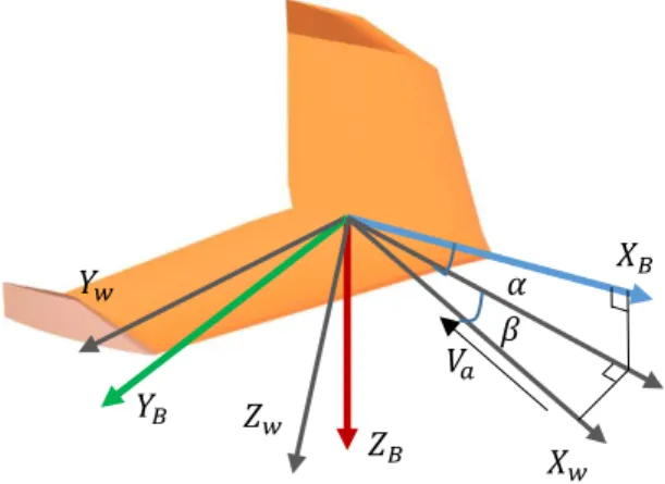
(2) [ , , ] T. A fixed wing is an unconventional type of aircraft with only two control surfaces (flaps) for manoeuvring (Figure 2). The symmetric deflection (  E ) of flaps will act in the control of the longitudinal motion variables (  , z ), and the asymmetric deflection (  A ) of flaps will act in the control of the lateral motion variables (  , ). The controlled attitude (, ), and heading () are further responsible of spatial displacement.. 𝐹𝑥 = 𝑚(𝑢̇ + 𝑞𝑤 − 𝑟𝑣) {𝐹𝑦 = 𝑚(𝑣̇ + 𝑟𝑢 − 𝑤𝑞) 𝐹𝑧 = 𝑚(𝑤̇ + 𝑝𝑣 − 𝑢𝑞). (1). where m is the plane mass. Euler’s second law on the angular momentum yields the contribution of the three torque components in the body frame: 𝑀𝑥 = 𝐼𝑥𝑥 𝑃̇ + (𝐼𝑥𝑥 − 𝐼𝑦𝑦 )𝑄𝑅 + 𝐼𝑥𝑧 𝑃̇ + 𝐼𝑥𝑧 𝑃𝑄 { 𝑀𝑦 = 𝐼𝑦𝑦 𝑄̇ + (𝐼𝑥𝑥 − 𝐼𝑧𝑧 )𝑃𝑅 + (𝑅2 + 𝑃2 )𝐼𝑥𝑧 , (2) 𝑀𝑧 = 𝐼𝑧𝑧 𝑅̇ + (𝐼𝑦𝑦 − 𝐼𝑥𝑥 )𝑃𝑄 + 𝐼𝑥𝑧 𝑃̇ − 𝐼𝑥𝑧 𝑄𝑅 being the inertial tensor:. Figure 2: Symmetric  E and asymmetric  A deflections.  I xx I   0  I zx. Linear [u, v, w]T and angular [ p, q, r ]T velocities of the fixed wing are measured in the body frame (B). Figure 3 depicts the three orthogonal axis of this second reference frame, which is clamped to the mass centre of the vehicle.. Parameters m A b c Va.  . 𝑉𝑎 𝑌𝐵. 𝑍𝑤. 𝑍𝐵. g kd kt Ixx Iyy Izz Ixz=-Izx. 𝑋𝐵. 𝛼 𝛽. I yy 0. I xz  0  I zz . (3). Mass and inertial moments for the fixed wing prototype in this work are in Table 1, together with other relevant parameters. Moments of inertia have been computed using the 3D simulation program XFLR-5 [4].. In all aerodynamic systems, special attention should be payed to the “wind frame” (W), whose X-axis is parallel to the air velocity vector Va . W reference frame involves a rotation  (attack angle) with respect to the body Y-axis and a rotation  (sweep angle) with respect to the body Z-axis, as Figure 3 illustrates. Va magnitude depends on the relative vehicle’s forward airspeed.. 𝑌𝑤. 0. 𝑰𝑿𝒋. Values 0.9 0.27 1 0.27 31 −0.5 0 −9.81 8.5 ∗ 10−9 5.65 ∗ 10−7 0.02381 0.00841 0.03222 0 2.44 ∗ 10−6. Units 𝑘𝑔 𝑚2 𝑚 m 𝑚/𝑠 º º 𝑚/𝑠 2 𝑁 ∙ 𝑚 ∙ 𝑠 2 /𝑟𝑎𝑑 𝑁 ∙ 𝑚 ∙ 𝑠/𝑟𝑎𝑑 𝑘𝑔 ∙ 𝑚2 𝑘𝑔 ∙ 𝑚2 𝑘𝑔 ∙ 𝑚2 𝑘𝑔 ∙ 𝑚2 𝑘𝑔 ∙ 𝑚2. Table 1. Parameters of fixed wing prototype and flight conditions. 𝑋𝑤. 2.2. Figure 3: Body clamped frame (colour) and wind frame (grey). External strengths and torques. The relative vehicle’s forward airspeed Va exerts an aerodynamic strength due to the variance of pressure. 2.1 Equations of motion in the body frame. 𝑄 = 12𝜌𝑉𝑎2 𝐴. Newton’s second law on the linear momentum yields the contribution of the three force components in the body frame:. 599. (4).

(3) between the upper and lower parts of the wing, whose surface is A;  is the air density. Thus, the drift (D), sweep (S) and lift (L) components of the aerodynamic strength in the wind frame are −𝐶𝐷 −𝐷 𝐅𝑎W = [ 𝑆 ] = 12𝜌𝑉𝑎2 𝐴 [ 𝐶𝑆 ], −𝐶𝐿 −𝐿. propeller 5051, all powered with a 4S LiPo battery. Propellers coefficients k t and k d in Table 1 have been experimentally identified according the procedure in [5]. The propeller rotation axis changes its orientation as the craft rotates. This induces a gyroscopic torque. (5). 𝐼𝑗𝑋 𝜔̇ 𝑗. being 𝐶𝐷 , 𝐶𝑆 , and 𝐶𝐿 the aerodynamic coefficients in each W axis. Then, the rotation matrix. 𝐑B←W = (. cosα cosβ sin β sin α cos β. 𝐌𝒈 = [ 𝐼𝑗𝑋 𝜔𝑗 𝑟 ] −𝐼𝑗𝑋 𝜔𝑗 𝑞. −cosα sinβ −sinβ cos β 0 ) ( 6) −sinα cos β cosα. where 𝐼𝑗𝑋 is the moment of inertia of the rotor around the X-body axe.. is applied to obtain those strengths in the body frame: 𝐹𝑎𝑋 𝐅𝑎 = 𝐑B←W 𝐅𝑎W = [𝐹𝑎𝑌 ] 𝐹𝑎𝑍. Finally, the craft weight in the earth frame responds to 0 𝐅𝒘𝐄 = [ 0 ] (12) −𝑚 𝑔. ( 7). where m is the mass of the aircraft and g is the gravity. Then, this force is conveniently rotated to the body frame giving. The application point of 𝐅𝑎 can slightly change depending on the attack  and sweep  angles. In order to simplify the problem, the application point is considered fixed and roll (L), pitch (M) and yaw (N) moments −𝑏 𝐶𝑙 𝐿 𝐌𝒂 = [𝑀] = 12𝜌𝑉𝑎2 𝐴 [ 𝑐 𝐶𝑚 ] −𝑏 𝐶𝑛 𝑁. −𝑚 𝑔 𝑠𝑖𝑛𝜃 𝐅𝒘 = [ 𝑔 𝑠𝑖𝑛𝜙 𝑐𝑜𝑠𝜃 ] 𝑔 𝑐𝑜𝑠𝜙 𝑐𝑜𝑠𝜃 2.3. (8). Non-linear model. rearranging, it yields the dynamic non-linear model of motion in the body frame: 2. and the angular velocities [ p, q, r ]T . Translational (5) and rotational (8) aerodynamic coefficients have been calculated following the equations in [3].. 𝑘𝑡 (𝑤𝑗 ). −𝑔 𝑠𝑖𝑛𝜃 +. 𝑚. 𝑔 𝑠𝑖𝑛𝜙 𝑐𝑜𝑠𝜃 + 𝑔𝑐𝑜𝑠𝜙 𝑐𝑜𝑠𝜃 −. A tail propeller rotates at j, which provides a thrust force along the X-body axis. 𝐼𝑗𝑋 𝜔̇𝑗 𝐼𝑥𝑥. 2. +. 𝑘𝑑 (𝑤𝑗 ). 𝐼𝑦𝑦. 1. +2. −𝐼𝑗𝑋 𝜔𝑗 𝑞. {. 𝐼𝑧𝑧. −. 𝐼𝑥𝑥. 𝐼𝑗𝑋 𝜔𝑗 𝑟. (9). to get the plane sustentation force. However, the friction between the propeller and the air also causes a parasitical drag moment around the X-body axis.  j = k d (  j )2 ,. (13). Substituting external forces and moments (Section 2.2) in generic forces and moments Fx , Fy , Fz , M x , M y , M z in (1) and (2), and. are added to correct this assumption; b and c are the wing span and chord, respectively; Table 1 details their values for this work prototype. 𝐶𝑙 , 𝐶𝑚 , 𝐶𝑛 are aerodynamic coefficients in each axis. They depend on the attack angle (), the flap deflection (  E ,  A ). T j = k t (  j )2. (11). 1. 𝑚. 𝐹𝑎𝑌 𝑚 𝐹𝑎𝑍 𝑚. + 𝑢𝑞 − 𝑣𝑝 = 𝑤̇. 𝐼𝑥𝑥. 𝐼𝑦𝑦 𝜌𝑉 2 𝑆𝑐𝑛 𝑏 𝐼𝑧𝑧. + 𝑣𝑟 − 𝑞𝑤 = 𝑢̇. + 𝑝𝑤 − 𝑟𝑢 = 𝑣̇. 1 𝜌𝑉 2 𝑆𝑐𝑙 𝑏 2. 𝜌𝑉 2 𝑆𝑐𝑚 𝑐. −2. 𝐹𝑎𝑋. −. − −. −. (𝐼𝑥𝑥 −𝐼𝑧𝑧 )𝑞𝑟 𝐼𝑥𝑥. (𝐼𝑧𝑧 −𝐼𝑥𝑥 )𝑝𝑟 𝐼𝑦𝑦. (14). = 𝑞̇. (𝐼𝑥𝑥 −𝐼𝑦𝑦 )𝑝𝑞 𝐼𝑧𝑧. = 𝑝̇. = 𝑟̇. The linear velocities [u, v, w]T can be transferred to the earth frame by multiplying them by matrix (see [5]). (10) 𝐑E←B = 𝐑E←B ∙ 𝐑E←B ∙ 𝐑E←B , 𝑥 𝑦 𝑧. which hampers the plane controllability. Thus, it is worth investing time to find the best motor-propeller combination. For this work prototype, we have opted for a motor Racestar BR2205, 2300Kv, with a 3-blade. (15). And after integration, it yields absolute position [x, y z]T. Expression (15) uses Euler angles that can be calculated integrating. 600.

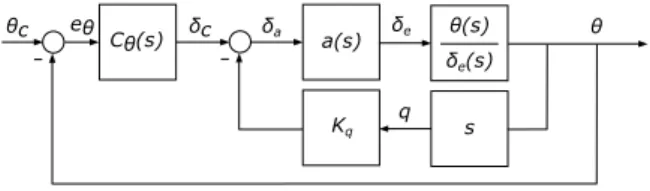
(4) 𝜙̇ 1 [ 𝜃̇ ] = [0 0 𝜓̇. 𝑠𝑖𝑛 𝜙 𝑡𝑎𝑛𝜃 𝑐𝑜𝑠 𝜙 𝑠𝑖𝑛 𝜙 𝑠𝑒𝑐 𝜃. 𝛼(𝑠) 𝛿𝐸 (𝑠). 𝑐𝑜𝑠 𝜙 𝑡𝑎𝑛𝜃 𝑝̇ − 𝑠𝑖𝑛 𝜙 ] ∙ [𝑞̇ ] (16) 𝑐𝑜𝑠 𝜙 𝑠𝑒𝑐𝜃 𝑟. 3.. In order to develop linear control laws, small signal linear models of (14) will be computed. The linearization process is about deriving the equations regarding all variant parameters, evaluating them on a nominal flight condition (Va=31 m/s, =-0.5º , =0º), and multiplying them by the sensitivity. The result of this process is commonly called stability derivatives in the aeronautic field. Longitudinal stability is used for pitch and height control, and lateral stability for roll and yaw control [3] [6].. In this work, two cascaded loops will allow controlling first the pitch angle. Then, considering the attack angle, it will allow controlling the height inside another outer loop. 3.1. 𝑈0 𝑀𝑢 + 𝑀𝑇𝑈 0 (. 0 𝑍𝑞 + 𝑈0. 𝑈0 𝑀𝛼 + 𝑀𝑇𝛼 0. 𝑈0 𝑀𝑞 1. −𝑔 0 0 0). 𝑢 𝛼 (𝑞 ) + 𝜃. Pitch control architecture. Figure 4 depicts the pitch control architecture. Block a(s) represents the actuator dynamic, which is here discarded (a(s)=1) in comparison with the rigid solid dynamics (s)/E(s). The pure derivative in the inner loop is actually a mathematical resource, since q is the measurable variable in practice. Thus, gain Kq is the controller in the feedback path of the inner loop. The outer loop provides the feedback controller C(s) in the direct path. The control design process is performed from the inner to the outer loop, as it is following detailed.. Only the strengths in X and Z axes, and the moments in Y axis will be studied, since they are the only ones deemed to intervene in longitudinal stability. With the coefficients obtained following [7], it yields the longitudinal linear model: 𝑋𝑎 𝑍𝛼. Control strategy. The desired attack angle is obtained by controlling a desired pitch angle, which finally will intervene in the altitude control. Similarly, a desired sweep angle is obtained by controlling a desired roll angle, which will intervene in the yaw control.. The longitudinal stability allows us to observe the behaviour of the linear velocity in X-axis (𝑢), the angle of attack (), the angular velocity in Y-axis (𝑞) -all them computed in the body frame- , and the pitch angle (  ) in the earth frame, which is approximated by the integration of the aforementioned angular velocity q under the assumption of small roll angles. The symmetric deflection of flaps  E is the actuation variable.. 𝑋𝑢 + 𝑋𝑇𝑈 𝑍𝑢. (20). In flight dynamics, it is all about controlling the magnitude and orientation of the lift vector. Thus, we will have to study those variables whose effect on the vector are significant. We find that the attack angle controls the magnitude and the sweep angle controls the orientation of the lift vector. Consequently, any manoeuvre of winning or losing height would start with a change in the angle of attack, in the same way that a change in the sweep angle has an inherited change in the lateral position.. Linear model: Longitudinal stability. 𝑢̇ 𝛼̇ ( )= 𝑞̇ 𝜃̇. −10.95 𝑠3 −2964 𝑠2 −569.6 𝑠−334.3 𝑠4 +30.37𝑠3 +3987𝑠2 +787.8 𝑠+658.7. are of interest in the longitudinal control strategies.. This also yields absolute orientation [ , , ] T.. 2.4. =. 𝑋𝛿𝐸 𝑍 𝛿𝐸 𝑈0 𝛿𝐸 𝑀𝛿𝐸 ( 0 ). (17) In particular, the state equation u 𝑢̇ −0.19 0 0 −9.17 0.51 α 𝛼̇ 0 −20.27 0.96 0 −11.05 ( )=( ) 𝛿𝐸 ) (q ) + ( 𝑞̇ 4.04 −3861.27−9.90 0 −2985.33 θ 0 0 1.00 0 0 𝜃̇. (18). Figure 4: Pitch control architecture. is obtained for the fixed wind prototype in this work. Accordingly, the following input-output transfer functions 𝜃(𝑠) 𝛿𝐸 (𝑠). From a pure mathematical point of view the diferenciator in the inner loop mitigates the underdamping (0.244) of dominant poles in (s)/E(s) of (19). Figure 5 depicts this effect in the frequency domain response of /E. Then, Kq is tuned to achieve a suitable control bandwidth BW; acceptable values are between 1 and 10 rad/s. Finally, a value of. −2985 𝑠2 −18820 𝑠−3487. = 𝑠4 +30.37𝑠3 +3987𝑠2 +787.8 𝑠+658.7 (19). 601.

(5) 𝐾𝑞 = −0.25. which achieves a PM of 90º at gc of 9.78 rad/s, as Figure 7 depicts. Finally, the closed-loop frequency response /c reaches -3dB above BW=5.5 rad/s.. (21). achieves a BW=1.71 rad/s, as Figure 6 shows. Let us remark that a negative control gain is necessary in the inner loop since (s)/E has inverse gain.. Figure 7: Open-loop frequency response of /e. 3.2 Figure 5: Open-loop frequency response /E. Altitude control architecture. The altitude control consists of another feedback control loop above the pitch control structure /c of Figure 4, as Figure 8 shows. C h (s) is the feedback controller to be designed. The path angle.  (t )   (t )   (t ). (23). is related to the altitude such that . h  U 0 sin   U 0 ,. (24). where U0 is the craft velocity that is equal to Va=31 m/s when ==0º.. Figure 6: Closed loop frequency response /c Regarding the outer loop design, a proportionalintegral (PI) controller is attempted: first, an integrator to remove the position error and later on a zero to mitigate the integrator effect over medium frequencies guaranteeing enough phase margin (PM) -higher than 40º-. The PI controller gain modulates the gain cross over frequency gc (values between 1 and 10 rad/s are acceptable). Negative control gain is necessary since /c has inverse gain as phase plot reveals in Figure 6. The final controller at the outer loop is (1 + 5s) C (s) = -0.632 s. Figure 8: Altitude control architecture Considering (23) (19) and (20), it is obtained  (s) -0.003667( s + 39.77)(s - 41.91)(s + 0.1727) ,(25) =  (s) (s + 6.115)(s + 0.191). which can be approximated by (s) 5.4189  (s) s  6.115. (22). (26). in order to simplify the design process. Finally, h/c presents the frequency response in Figure 9.. 602.

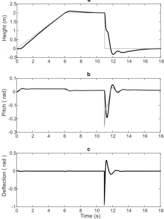
(6) aforementioned control loops (Sections 3.1 and 3.2) have been also implemented in the script. Besides, yaw must be controlled to zero, using a similar control structure (Figure 11) as in the height control, let us note as it includes inner roll control loops, similar to the pitch control architecture.. A PI controller cannot achieve acceptable PM (above 45º) for good stability and high enough cross overfrequencies (1-10 rad/s) for a good performance. However, the final controller Ch ( s) . 0.05 (1  s / 0.9)( s  1) s (1  s / 2.4). (27). achieves a PM of 51.45º and cg=2.54 rad/s as Figure 10 shows. The closed-loop bandwidth of h/hc is BW=4.25 rad/s.. Figure 11: Yaw control architecture Figure 12 depicts several time responses related to height reference changes of step and ramp type. Plot (a) depicts the height tracking response (black) to reference signals (grey) of different nature; plot (b) shows the pitch that is demanded (grey) and how it is attained (black) by the inner loop; and plot (c) shows the deflection angle variation.. Figure 9: Frequency response of h/c. Figure 12: Altitude control performance. Figure 10: Open-loop frequency response of h/eh 3.3.. Validation in the non-linear model. 4. Longitudinal control is being tested in the fully coupled system with all the non-linear behaviours. The non-linear model in Section 2.3 has been implemented in a “User-Defined Block” in Simulink with the symmetric and asymmetric flap deflection as control inputs, and the three Euler Angles and altitude as controlled outputs. Using this block, the. Conclusions. In this article, we have presented the mathematical model of a fixed wing aircraft. For a hand-made protype, we have identified aerodynamic and physical parameters such as aerodynamic coefficients, inertias or weights, among others, mainly using the opensource software XFLR-5. Furthermore, we have. 603.

(7) isolated all the moments and strengths in the system: weight, aerodynamic forces and moments, thrust, drag sweep.. [2] Alexander V. Koldaev. (2007) “Non-military UAV applications”. [3] David K. Schmidt. (2012) “Modern Flight Dynamics”, McGraw-Hill International Edition.. Following Newton-Euler formulation, we have come up with a non-linear model, which has been linearized in order to apply linear control theory.. [4] Guidelines for XFLR5 V0.03. (2009) “XFLR5 Analysis of foils and wings operating at low Reynolds numbers”.. A longitudinal stability model has been used to design feedback control loops of a cascade structure. Frequency domain techniques were used to design PID type controllers. An inner feedback loop controlled the pitch angle by conveniently acting on the flap deflection. Then, an outer loop allowed tracking the desired altitude.. [5] R.Rico, P. Maisterra, M. Gil-Martínez, J. RicoAzagra, S. Nájera (2015). “Identificación experimental de los parámetros de un cuatrirrotor”. In XXXVI Jornadas de Automática.. Achieving this controlled model is the start of a way for improvement and allows us to contribute to the creation of navigation systems, laying the foundations of new work lines.. [6] Smetana, Frederick O. Delbert C. Summery and W. Donlad Johnson (1972), “Riding and Handling Qualities of light Aircraft-A Review and Analysis”. National aeronautics and space administration. Washington D.C. The development of the model and its control is the first step to design optimized control strategies and to explore new possibilities in the field.. [7] Esteban. S., (2001) “Static and dynamic analysis of an unconventional plane: Flying wing”. In AIAA Atmospheric Flight Mechanics Conference and Exhibit.. Acknowledgements The authors gratefully appreciate the support given by La Rioja Government under grant ADER 2017-I-IDD00035 and the support given by the University of La Rioja under grant REGI 2018/42. References. © 2018 by the authors. Submitted for possible open access publication under the terms and conditions of the Creative Commons Attribution CC-BY-NC 3.0 license (https://creativecommons.org/licenses/by-nc/3.0).. [1] Mark Edward Peterson. (2006) “The UAV and the current and future regulatory construct for integration into the national airspace system”. Journal of Air Law and Commerce, vol. 71(5) pp. 521-612.. 604.

(8)