A methodology for predicting the energy performance and indoor thermal comfort of residential stocks on the neighbourhood and city scales A case study in Spain

Texto completo

(1)Title page Title A methodology for predicting the energy performance and indoor thermal comfort of residential stocks on the neighbourhood and city scales. A case study in Spain. Authors names and affiliations a. a. a. Marta Braulio-Gonzalo *, María Dolores Bovea , María José Ruá , Pablo Juan. b. a. Department of Mechanical Engineering and Construction, Universitat Jaume I, Av. Sos Baynat s/n, 12071 Castellón, Spain b. Department of Mathematics, Universitat Jaume I, Av. Sos Baynat s/n, 12071 Castellón, Spain. Marta Braulio-Gonzalo Name:. Marta (M.). Surname:. Braulio-Gonzalo. E-mail address: braulio@uji.es. María D. Bovea Name:. María D. (M.D.). Surname:. Bovea. E-mail address: bovea@uji.es. María José Ruá Name:. María José (M.J.). Surname:. Ruá. E-mail address: rua@uji.es. Pablo Juan Name:. Pablo (P.). Surname:. Juan. E-mail address: juan@uji.es. *Corresponding author Marta Braulio-Gonzalo Tel. +34 964 729162 E-mail address: braulio@uji.es Universitat Jaume I, Department of Mechanical Engineering and Construction, Av. Sos Baynat s/n, 12071 Castellón, Spain. 1.

(2) Title A methodology for predicting the energy performance and indoor thermal comfort of residential stocks on the neighbourhood and city scales. A case study in Spain. Abstract The aim of the study is to present a developed bottom-up-based methodology for predicting the energy performance of residential stocks on the neighbourhood and city scales. This methodology enables predicting the energy demand and discomfort hours (heating and cooling) taking into account urban and building factors such as urban block type, street heightwidth ratio and solar orientation of the main façade, and shape factor and year of construction of the building, respectively. For this purpose, a four-staged methodology consisting in (1) urban taxonomy characterisation, (2) energy performance assessment, (3) statistical modelling and (4) stock aggregation is proposed, which combines building physical modelling and statistical inference in a Geographical Information System environment to provide an intuitive visual interface that represents final results on urban energy maps. The methodology was implemented in a medium-sized Spanish Mediterranean city as a case study, which allowed estimating the passive energy performance of a neighbourhood and setting building and urban design strategies. Results allowed concluding that the intrinsic parameters of the urban morphology play an important role on passive energy performance and important energy demand savings can be achieved when considering morphological urban aspects in new planning developments. This methodology is an efficient tool that can help stakeholders and local authorities in decision-making processes that focus both on developments of new urban areas taking into account energy requirements and on identifying and prioritising existing residential stocks in need of rehabilitation in energy terms.. Keywords: passive energy performance; residential building stock; urban morphology; GIS; bottom-up model; INLA. 2.

(3) Abbreviations CREEM BREHOMES UKDCM DECarb EEP CDEM DECM TABULA SLABE. The Canadian Residential Energy End-use Model; Building Research Establishment Housing Model for Energy Studies UK Domestic Carbon Model future climate data and current housing stock data for the UK Energy and Environment Prediction Community Domestic Energy Model Domestic Energy and Carbon Model Typology Approach for Building Stock Energy Assessment Simulation-based Large-scale uncertainty/sensitivity Analysis of Building Energy performance TIMES The Integrated MARKAL-EFOM System QuBEC Quantitative Evaluation of European Building Stock Energy Consumption Using a Novel Application of CHAID analysis ECCABS Energy, Carbon and Cost Assessment for Building Stocks. BREDEM BRE Domestic Energy Model GIS Geographical Information System SHEU Survey of Household Energy Use, Canada statistics RECS Residential Energy Consumption Survey IMPRO-Building Environmental Improvement Potentials of Residential Buildings, European Commission DECADE Domestic Equipment and Carbon Dioxide Emissions, University of Oxford NHSS National Hellenic Statistical Service, Greece SACE Sistema accreditamento certificazione energetica degli edifici, Emilia-Romagna region EEM Energy Efficiency Measures BAG Basisregistraties Adressen en Gebouwen. INLA Integrated Nested Laplace Approximation Subscripts h c. heating cooling. 3.

(4) 1. Introduction The sustainable urban development is an emerging trend in our cities and in the built environment in general (De Jong et al., 2013; Yin et al., 2015). The path towards urban sustainability requires the diagnosis of the current built environment as a starting point in order to be able to define informed policy initiatives to promote sustainable urban development. Many aspects are involved in urban sustainability, such as mobility and transport, building and housing, waste, pollution, socio-economic or institutional, but energy issues related to the building sector are identified as one of the key aspects (Braulio-Gonzalo et al., 2015a). In this context, there is a growing consensus about the need to assess the energy use of the building stock of residential areas (Uihlein and Eder, 2010). Swan and Ugursal (2009) and Kavgic et al. (2010) reviewed the modelling techniques used to predict residential energy consumption, and identified two different approaches: bottom-up and top-down. The topdown approach, based on macro-economic indicators such as price, income and climate data, treats the residential sector as an energy sink. So it is not concerned about individual end uses and is unable to identify areas in need of energy performance improvement. In contrast, the bottom-up approach extrapolates the estimated energy use of a representative set of individual buildings at regional and national levels by conducting stock aggregation. This approach is based on more detailed and accurate building information and then confers the ability to model different technological options. Two distinct techniques are applied in bottomup models, depending on input data and structure: statistical and building physics (engineering). By modelling the energy performance of residential stocks, entire urban areas can be assessed and those influential aspects can be identified. Energy performance of buildings has a great deal on the intrinsic design aspects of the built environment, such as urban morphology and physical context of the surroundings. Then, previously to implement active measures to improve the energy efficiency in buildings, an accurate urban and building design may help ensure lower energy demands in residential stocks and achieve more energy-efficient urban planning by only considering passive energy strategies. For instance, Salat (2009) summarised some factors that vary extensively depending on urban layout and highlighted that they all strongly influence the energy performance, such as building shape factor, density, porosity, light and natural ventilation, and a building’s envelope performance. Thus, design strategies should be defined in the early stages of urbanisation processes so that stakeholders have tools 4.

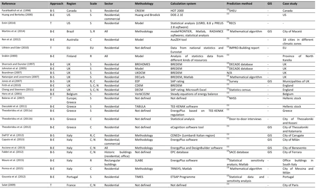
(5) to obtain information about the influence of design variations on the energy performance of building stocks (Granadeiro et al., 2013). In this sense, bottom-up approach facilitates the identification of sensitive variables on the overall energy performance, which allows, by changing such variables, to forecast the results of specific scenarios and to prepare substantive arguments for particular building designs and policies (Moffatt, 2001). Several authors have developed methods to make energy assessments of building stocks, whose main characteristics are presented in Table 1. The scope covered by these studies is diverse, and ranges from the state scale to the neighbourhood scale. As seen, it is outlined that most reviewed studies have been based in a bottom-up approach, except for (Balaras et al., 2007; Estiri, 2014; Salat, 2009; Uihlein and Eder, 2010), which have been conducted within a top-down framework.. 5.

(6) Table 1. Review of the methods whose aim is the energy assessment of building stocks Reference. Approach. Region. Scale. Sector. Methodology. Calculation system. Prediction method. GIS. Case study. Farahbakhsh et al. (1998) Huang and Berkeley (2000). B-S B-E. Canada US. S S. CREEM Huang and Brodick. HOT 2000 DOE-2.1E. (2). SHEU. -. Canada US. Estiri (2014). T. US. S. Residential Residential; commercial Residential. Model. (2). RECS. -. -. Martins et al. (2014). B-E. Brazil. S; R. All. Methodology. GIS. City of Maceió. Ren et al. (2012). B-E. Australia. C. Residential. Model. Statistical analysis (LISREL 8.8 y PRELIS 2.8 software) modeFRONTIER, Matlab, RADIANCE softwares; statistical analysis AusZEH tool. (1). -. Data from national statistics and Eurostat Analysis of statistics data from different kinds of resources BREDEM BREDEM BREDEM BREDEM, Matlab SAP rating BREDEM SAP rating; Microsoft Excel Steady equations of energy balance Not defined. (2). -. 18 cities in different climatic zones EU. (1). -. (2). GIS -. Province of North Karelia UK UK UK UK Municipalities of UK England England Belgium Hellenic stock. (1). -. Hellenic stock Greece. -. Uihlein and Eder (2010). T. EU. EU. Residential. Not defined. Snäkin (2000). B-E. Finland. R. All. Model. Shorrock and Dunster (1997). Theodoridou et al. (2011b). B-S. Greece. C. Residential. Not defined. TEE-KENAK software EnergyPlus based on regulation Statistical analysis. Theodoridou et al. (2012). B-E. Greece. C. Residential. Not defined. eCognition software tool. (1). GIS. Methodology Methodology. CENED+ (Lombardi Italian region) EnergyPlus software. (1). GIS GIS. City of Thessaloniki and Kozani City of Thessaloniki and Kalamaria City of Carugate City of Milán. Methodology Not defined. EnergyPlus and DesignBuilder software EPC database. (1). GIS GIS. City of Benevento City of Ferrara. SLABE. EnergyPlus software. (3). -. Methodology. TRNSYS; Matlab. Statistical sensitivity analysis; Matlab (3) Mathematical algorithm. -. Office buildings in South Italy City of Messina and Milán Portugal. -. City of Paris. Balaras et al. (2007) Dascalaki et al. (2011). Dall’O’ et al. (2012). BREHOMES Model UKDCM DECarb EEP CDEM DECM VerbCO2M Not defined. S S. Residential Residential. TABULA Not defined. IMPRO-Building report. B-E B-E. Cheng and Steemers (2011) Hens et al. (2001). Residential Residential Residential Residential Residential Residential Residential Residential Residential. Mathematical algorithm. Theodoridou et al. (2011a). Natarajan and Levermore (2007) Jones et al.(2007) Firth et al.(2010). S S S S R; C S; C; N S; C; N S S. (3). UK UK UK UK UK UK UK Belgium Europe; Greece Greece Greece. Johnston et al. (2005) Boardman (2007). B-E B-E B-S B-S B-S B-E B-E B-E T. (1). Caputo et al. (2013). B-S B-E. Italy Italy. R; C C; N. Ascione et al. (2013) Fabbri et al. (2012). B-E B-S. Italy Italy. C; N C; N. Mauro et al. (2015). B-E. Italy. R. Penna et al. (2015). B-E. Italy. C. Residential Residential; commercial All Historic buildings (residential, office) Rectangular buildings Residential. TEE-KENAK. DECADE database DECADE database N/A (3) Mathematical algorithm (2) Survey (2). (1) (2). (2). NHSS. (1). (2). Door-to-door interviews. (1). (2). Gouveia et al. (2012). B-E. Portugal. S. Residential. TIMES. ETSAP Programme. (2). Salat (2009). T. France. C; N. Residential. Not defined. Not defined. (1). 6. Statistics census. (1). SACE database. Statistical data sensitivity analysis. and. -.

(7) Florio and Teissier (2015) Fonseca and Schlueter (2015). B-E. Switzerland. S; R C; N. Residential. TABULA. All. (3). -. France. (1). GIS. Neighbourhood of Zug. (2) (3). GIS -. City of Basilea Sweden. (1). -. Statistical analysis. B-S B-E. Switzerland Sweden. N S. All Residential. QuBEC ECCABS. McKenna et al. (2013) Košir et al. (2014). B-S B-E. Germany Slovenia. S C; N. Residential Residential. Model Not defined. Data form different sources SHADING software. Terés-Zubiaga et al. (2013). B-E. Spain. C. Not defined. Energy bill surveys; building monitoring. (1). -. Germany Different municipalities City of Bilbao. Not defined TABULA. LIDER software CERMA software. (1). -. Catalonia -. Methodology. EN ISO 13790:2008. (3). B-E B-E. Spain Spain. R S. B-E. Germany. C; N. Residential. (social. SIA;. sensitivity. Aksoezen et al. (2015) Mata et al. (2013). Residential housing) Residential Residential. Model. Algorithm and EPC French database ECS (EN ISO); TRANSYS, EnergyPlus; statistical analysis Real gas consumption data Simulink software. Garrido-Soriano et al. (2012) Instituto Valenciano de la Edificación (2014) Camargo-Ramirez (2012). B-E. France. Statistical analysis Treatment of results with Matlab software Not defined. (1). Statistical sensitivity GIS analysis (2) Laubinger (2015) B-S Netherlands C Residential Methodology BAG database Statistical sensitivity GIS analysis B-S: Statistical bottom-up approach; B-E: Engineering bottom-up approach; T: Top-down; EU: European Union; US: United States; UK: United Kingdom; S: State; R: Regional; C: City; N: Neighbourhood (1) Aggregation; (2)Database relay; (3)Complex prediction method. 7. City of Grafenau Amsterdam. Freyung-.

(8) As shown in Table 1, most of the reviewed studies have considered a wide range of variables that focus on the specificities of the region, such as ad hoc developed methodologies and software based on country regulations. However, they have not all combined distinct technologies to enhance the accuracy of their method. In fact, Kavgic et al. (2010) had already exhaustively reviewed different techniques for modelling energy consumption in the residential sector by a bottom-up approach. Yet after a critical analysis, they have also outlined the increasing need to continue developing more sophisticated building stock models, especially those that incorporate multidisciplinary aspects. The present study proposes a bottom-up-based methodology for predicting the energy performance and indoor thermal comfort of residential stocks on the neighbourhood and city scales. It is based on a complex prediction method that combines building physics modelling and statistical inference in a GIS environment, which provides an intuitive visual interface that represents the final results on urban energy maps. The engineering technique is based on building dynamic thermal simulation. The statistical inference is based on the Integrated Nested Laplace Approximation (INLA) (Rue et al., 2009), which enables the response variables in all the buildings that compound the residential stock under study to be individually estimated. Finally, the aggregation of individual results allows conclusions on an urban scale to be extrapolated. The paper is structured as follows: Section 2 presents the proposed methodology, which includes the selection of response variables and covariates based on a literature review, and describes the four stages that comprise it. Section 3 addresses the application of the methodology in a neighbourhood of Castellón de la Plana (east Spain). In Section 4, the influence of the urban and building covariates on the response variables is analysed, which allows a new planning proposal to be drawn and its energy assessment in Section 5. Finally, Section 6 offers the discussion and conclusions of the study.. 2. Methodology The methodology proposed herein enables an estimate of the energy demand (EDh and EDc, heating and cooling, respectively) and discomfort hours (DHh and DHc, heating and cooling, respectively) related to a residential stock according to its energy features. The application of this methodology enables the prediction of the passive energy performance of a stock and the identification of the most influential factors. In addition, the integration of INLA allows the key variables that affect building thermal performance to be identified. This allows the definition of a set of urban design strategies for decision making during new urban development designs and urban regeneration. 8.

(9) projects, and helps improve energy performance and then reduce the energy demand of residential stocks. The literature review shows that an appropriate methodology for evaluating the energy use of building stocks should be based on a bottom-up approach. Taking into account the conclusions drawn from the review, the following requirements were selected to be considered in the proposed methodology: A. Be adaptive to an urban context B. Be based on a passive energy assessment C. Consider building and urban parameters D. Use dynamic simulation E. Use statistical modelling. F. To be developed in a GIS environment 2.1 Selection of response variables and covariates By focusing on those reviewed studies based on a bottom-up approach, a more in-depth analysis has been done by analyzing the passive aspects considered in each one. The referred studies are reported in Table 2 and classified into energy assessment variables and influential aspects on the energy performance of building stocks, which resulted in a set of response variables and covariates, respectively.. 9.

(10) Table 2. Passive variables considered in the reviewed bottom-up models Influential aspects on the energy performance of building stocks Building. • • • • • • • • •. • • • •. • • • • •. • • • •. • • •. • • •. • •. • •. • •. • • • • •. • • •. • • •. • • •. • •. • •. •. •. •. • • •. •. •. •. • •. • • • •. •. •. • • • • •. • •. •. •. • •. Discomfort hours (DH). • •. Energy demand (ED). U-values windows. • • • •. Envelope transmittance. U-values opaque envelope. Built area. Shape factor (S/V). Building typology. Solar orientation. Street H/W ratio. Model CREEM (Farahbakhsh et al., 1998) Huang and Berkeley (2000) Ren et al. (2012) Snäkin (2000) BREHOMES (Shorrock and Dunster, 1997) Johnston et al. (2005) UKDCM (Boardman, 2007) DECarb (Natarajan and Levermore, 2007) EEP (Jones et al., 2007) CDEM (Firth et al., 2010) DECM (Cheng and Steemers, 2011) VerbCO2M (Hens et al., 2001) TABULA (Dascalaki et al., 2011) Dall’O’ et al. (2012) Caputo et al. (2013) Ascione et al. (2013) SLABE (Mauro et al., 2015) Penna et al. (2015) TIMES (Gouveia et al., 2012) TABULA (Florio and Teissier, 2015) Fonseca and Schlueter (2015) QuBEC (Aksoezen et al., 2015) ECCABS (Mata et al., 2013) McKenna et al. (2013) TABULA (Instituto Valenciano de la Edificación, 2014) Camargo-Ramirez (2012) Laubinger (2015) Considered in this work. Urban morphology. Compactness. Year of construction. Urban. Energy assessment variables. • • • •. • • •. • • •. • •. • •. •. •. •. •. •. Most of the developed models focused on variables that implied the consideration of active thermal systems to estimate energy consumption, CO2 emissions, cost or energy ratings. However, those that analysed energy performance from a passive point of view are scarcer. Although energy demand is considered more widely, very few include the assessment of thermal comfort conditions inside the building, which provides an accurate diagnosis of passive energy performance. Nevertheless, previous work has been done on indoor thermal comfort analyses. Mavrogianni et al. (2012) explored the impact of building factors, such as dwelling archetype, morphology of external environment, orientation and envelope U-values, on indoor summer temperatures in London dwellings. They concluded that the combination of built form and construction age accounted for an appreciable degree of variation in daytime living room temperatures, and that insulation interventions appeared to reduce the overheating risk for the stock. Singh et al. (2016) conducted 10.

(11) long-term monitoring of the indoor environment in Belgian residential buildings in combination with comfort surveys that recorded occupants’ adaptive actions to support the conclusions. The study showed that occupant behaviour and family composition strongly affected the functioning and occupant preferences for indoor thermal environments, and that occupants' adaptations markedly affected the energy consumption and overall energy efficiency of the house. Despite the existence of some work done in the thermal comfort field, only three bottom-up models (SLABE (Mauro et al., 2015), Penna et al. (2015) and TIMES (Gouveia et al., 2012)) have included it as an energy assessment variable. As for the passive influential aspects on energy performance, most models focus on building parameters related to building compactness and envelope thermal transmittance. Those aspects related to urban layout have been poorly approached. Only solar orientation has been integrated into three models (Ascione et al., 2013; Caputo et al., 2013; Mauro et al., 2015). Nevertheless, solid evidence for the influence of urban morphology and the street H/W ratio on the energy performance of buildings has been found in the literature. Futcher and Mills (2013) pointed out that the role of urban layout on the energy performance of buildings is often overlooked, even though it can greatly influence a building’s heating and cooling requirements (Capeluto, 2003; Košir et al., 2014). Oke (1988) outlined urban geometry to be a key factor to study solar access, and defined the sunlit area percentage in a wall that faced south for a range of H/W ratios (street height-width ratio) and latitudes. Along the same lines, Martins et al. (2014) proposed the distance between buildings on N-S and E-W axes as a constraint to analyse solar opportunities on buildings façades. Finally, Yezioro et al. (2006) examined insolation on façades oriented towards courtyards in 12 urban squares with different proportions (lengths, widths and heights). Accordingly, it can be concluded that urban layout aspects increasingly gain importance besides traditional building aspects when analysing the energy assessment of the building stock. Based on this analysis, a set of response variables and a set of covariates were selected, as detailed below. Four response variables were the key parameters considered to assess the energy performance of the residential building stock: . Energy demand for heating (EDh) and energy demand for cooling (EDc). Both variables measure the amount of energy that the thermal installations of the building have to provide in order to ensure inner comfort conditions according to building use and climatic zone (CTE, 2013) for heating and cooling, respectively. They are expressed as kWh/m2·year.. 11.

(12) . Discomfort heating hours (DHh) and discomfort cooling hours (DHc). They are the equivalent to ASHRAE unmet load hours and measure the time when the combination of zone humidity ratio and operative temperature is not in the ASHRAE 55-2004 summer or winter clothes region (DesignBuilder UK, 2015a) for heating and cooling, respectively. They are expressed as h/year.. These response variables mainly depend on the performance of five parameters related to the building or city scale, which are considered as covariates in this study. These are the following: . UB. Urban block refers to the geometry of the urban layout where the building is placed. And defines the typical block patterns in a city, which represent the smallest urban unit that includes not only individual buildings, but also a set of buildings that perform energetically as a whole.. . H/W. The dimensions of the public space can be described by the street height-width ratio, which represents the relation between the height of the buildings placed in front of the building under study and street width, and is responsible for solar access into the buildings surrounding the built environment. Higher H/W ratios imply more shaded streets and, therefore, less solar access opportunities for surrounding buildings.. . O. Solar influence has different affects depending on the latitude, so it is an important point to be explored in the specific region under study.. . S/V. Shape factor is defined as the ratio of a building’s total external surface area (S) to its inner volume (V) (Granadeiro et al., 2013). This was chosen to represent building class since it can be expressed by a numerical coefficient. This coefficient quantifies the building’s envelope surface exposed to the outdoor environment, and then represents the exchanging heat of the building with the exterior, which is strongly related to the urban fabric and urban density (Aksoezen et al., 2015). Lower S/V values mean more compact buildings in relation to higher energy efficiency.. . Y. Year of construction is related to the U-values of thermal envelope elements and can be standardised per construction period, which respond to thermal regulation milestones and historical and economic facts. It helps identify construction materials and the level of insulation employed to execute the building.. 12.

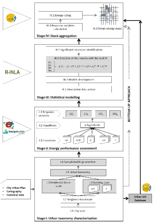
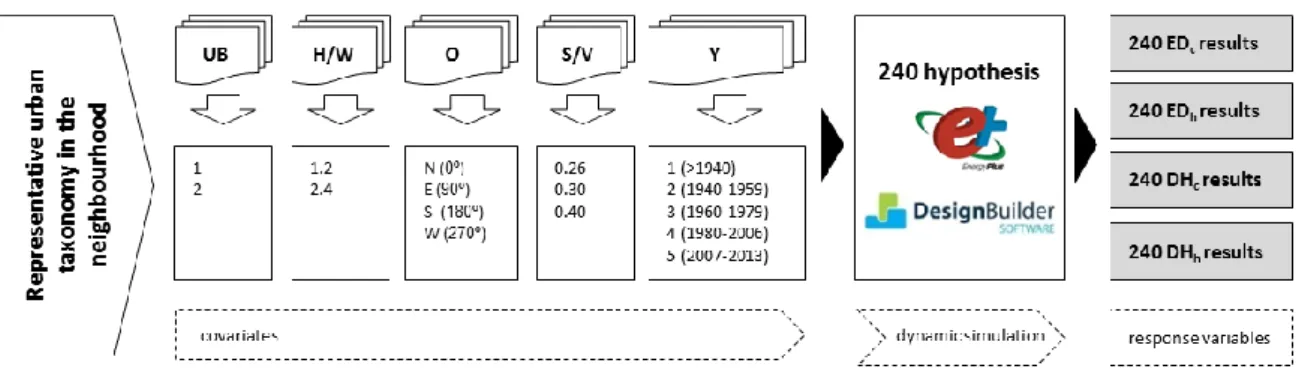
(13) 2.2 Stages of the methodologyThe methodological framework consists in four main stages, which are graphically described in Figure 1, from the bottom (Stage I) to the top (Stage IV). The shaded text boxes represent the main results obtained in each stage and examples of the specific software, which can be used to develop each stage, are indicated to the left of Figure 1 by their logos.. Figure 1. Methodological framework . Stage I: urban taxonomy characterisation. The residential building stock is broken down into an urban taxonomy on four different scales: city, neighbourhood, residential block and building 13.

(14) scale (Braulio-Gonzalo et al., 2015b). The City Urban Plan, the cartography and cadastral data, should be collected and used as input information to obtain the urban taxonomy. GIS is extremely useful in this stage because it helps create an urban GIS database that is also valuable in later stages of the methodology. A set of values for the covariates should be defined, specifically for the urban area under study. As a result of this stage, residential block types and building classes that exist in the neighbourhood are identified, as are the covariates included on each scale. Thus, representative building samples can be selected to be energy-modelled. . Stage II: energy performance assessment. Representative buildings of each class are selected and modelled in the residential urban block context. By combining all the covariates (UB, S/W, O, S/V and Y), a set of hypothesis is obtained. Running each hypothesis as an independent simulation allows four response variables of the method (EDc, EDh, DHc and DHh) to be determined for each single hypothesis. This stage should be conducted by using dynamic building simulation software.. . Stage III: statistical modelling. The results obtained in Stage II are processed and statistically in order to predict the response variables of the existing residential building stock by considering the five covariates, and to conduct a sensitivity analysis that allows the key covariates that affect the response variables to be identified. To do so, Bayesian inference was applied by using the Integrated Nested Laplace Approximation (INLA) methodology, developed by Rue and Martino (2007), and subsequently improved by Rue and Martino (2009). INLA delivers an integrated approach to make predictions and decisions. This method can be considered a global sensitivity analysis method according to the classification for building energy analyses proposed by Tian (2013). The general structure of the equations is: i  0   1 X i i. where.  0 is a scalar that represents the intercept, and   1 ,...,  M  are coefficients of. the linear effects of covariates. z  z1 ,..., zM  on the response. The effect of each covariate. on the response variables can be quantified. As a result, one equation per response variable is obtained, depending on the covariates. . Stage IV: stock aggregation. Once the algorithms for the response variables have been obtained, individual buildings in the urban area can be energy-assessed by predicting energy demand and discomfort hours according to the building and urban parameters (values of covariates). Then the results of individual buildings can be aggregated upwards and used to assess the energy performance of the residential building stock by a bottom-up approach. GIS technology provides. 14.

(15) graphical representations of results through urban energy maps and, finally, an energy class scale should be defined in order to graphically represent the results obtained.. 3. Application of the methodology: a case study in Spain The methodology was applied to Castellón de la Plana, a medium-sized city with 180,690 inhabitants (INE, 2015) located on the east Mediterranean coast of Spain. This city is located at 39° 59’ 11” north latitude and 0° 2’ 12” east latitude. According to CTE (2013), Castellón de la Plana belongs to climatic zone B3, characterised by a mild climate with temperate winters and warm summers. The aim of the case study was to conduct the energy characterisation of a neighbourhood in the city based on the analysis of representative buildings herein. The selected neighbourhood is representative of the urban layout in the city (Braulio-Gonzalo et al., 2015b) and is highlighted in Figure 2.. Figure 2. Castellón de la Plana’s historical evolution according to year of construction and identification of the selected neighbourhood. 3.1. Stage I: urban taxonomy characterisation On the city scale, the urban layout of the city was examined after considering the historical evolution and the Urban Plan. Figure 2 shows the city’s urban evolution on a GIS map. Here we can see that neighbourhoods result in urban areas linked to the year of construction of buildings according to the 15.

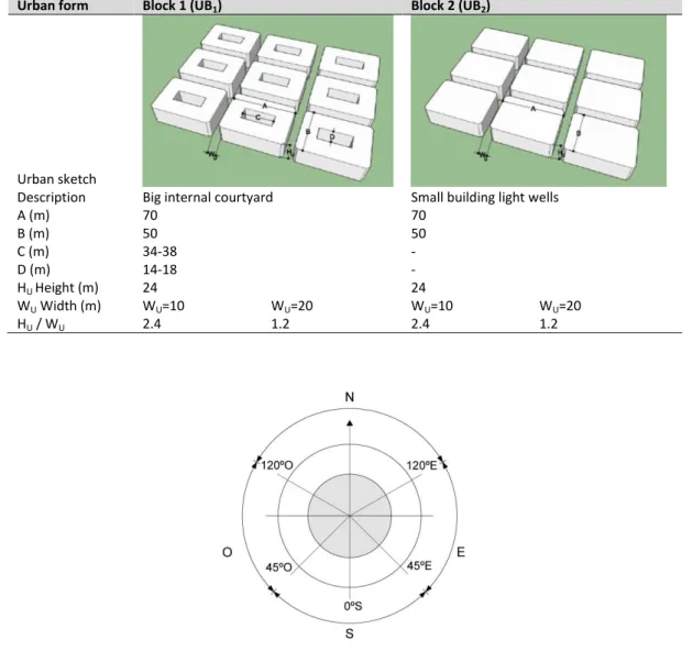
(16) city’s evolution. The GIS database contains data, such as type of building, number of floors, year of construction, built area and land surface, which were provided by the General Cadastre Office of Spain (DGC, 2014), and it enables the characterisation of the residential building stock. After contextualising the urban layout of the city, a representative neighbourhood with a wide variety of building typologies built during different construction periods was selected (Figure 2). This neighbourhood lies west of the city and corresponds to an expansion district with an orthogonal-grid urban layout that dates back to the 1930s. Two residential block types were identified in the neighbourhood. Although both blocks are similar in size (70 m long, 50 m wide, 24 m high), they present different internal structures due to the configuration of courtyards. Block type 1 (UB1) has a big internal courtyard that allows solar gains on the south, east and west façades of the buildings, with an inward orientation towards the courtyard. In contrast Block type 2 (UB2) does not have a big courtyard, but smaller light wells that act as internal building elements. The latter does not offer the possibility of significant solar gains for natural lighting and heating as a bigger courtyard does. Table 3 shows both residential urban block types and their dimensional properties. The maximum building height established by the City Urban Plan is eight floors above ground level (24 m) and two street widths exist in the neighbourhood (10 m and 20 m wide). The combination of both parameters determines two street height/width ratios (H/W). The orientation of the main façade of the buildings is represented by the angle defined by the perpendicular axis of the façade with the geographic north, and is measured in degrees according to Figure 3.. 16.

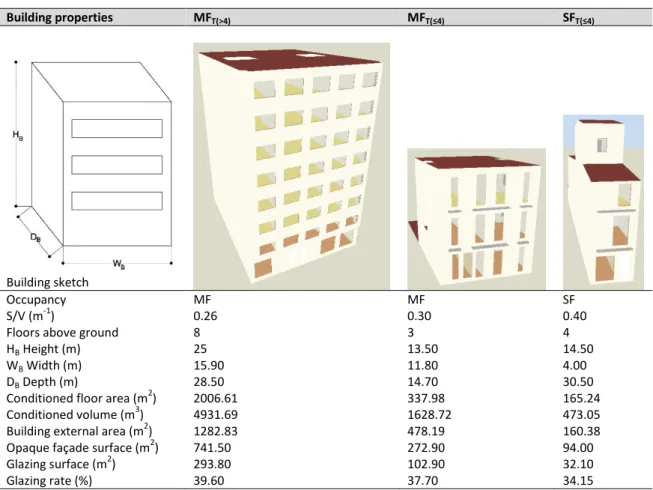
(17) Table 3. Residential urban block (UB1 and UB2) properties Urban form. Block 1 (UB1). Block 2 (UB2). Urban sketch Description A (m) B (m) C (m) D (m) HU Height (m) WU Width (m) HU / WU. Big internal courtyard 70 50 34-38 14-18 24 WU=10 WU=20 2.4 1.2. Small building light wells 70 50 24 WU=10 WU=20 2.4 1.2. Figure 3. Orientation of the building’s main façade based on the Spanish regulations framework (CTE, 2013) As for the building scale, three terraced building types (MFT(≤4), MFT(>4) and SFT(≤4)) were identified in the neighbourhood according to their occupancy (single-family, SF, or multi-family, MF) and number of floors (≤4, or > 4), as Table 4 reports. Building class was transformed into the shape factor coefficient (S/V), with MFT(>4) corresponding to 0.26, MFT(≤4) to 0.30 and SFT(≤4) to 0.40.. 17.

(18) Table 4. Properties for building classes MFT(>4), MFT(≤4) and SFT(≤4). Building properties. MFT(>4). MFT(≤4). SFT(≤4). Building sketch Occupancy -1 S/V (m ) Floors above ground HB Height (m) WB Width (m) DB Depth (m) 2 Conditioned floor area (m ) 3 Conditioned volume (m ) 2 Building external area (m ) 2 Opaque façade surface (m ) 2 Glazing surface (m ) Glazing rate (%). MF 0.26 8 25 15.90 28.50 2006.61 4931.69 1282.83 741.50 293.80 39.60. MF 0.30 3 13.50 11.80 14.70 337.98 1628.72 478.19 272.90 102.90 37.70. SF 0.40 4 14.50 4.00 30.50 165.24 473.05 160.38 94.00 32.10 34.15. By applying the gvSIG software (Asociación gvSIG, 2014), a neighbourhood can be graphically represented as a combination of building shape factors and block types, as Figure 4 shows. To address this, urban data were obtained after thoroughly processing the census information provided by DGC (2014) in the city.. 18.

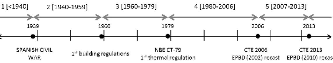
(19) Figure 4. Example of the identification of covariates UB and S/V in the analysed neighbourhood In order to run the simulations, the U-values of the typical constructive elements of the building (façade, roof, floor, internal partitions and fenestration) had to be determined. For this, buildings were categorised in five time periods according to year of construction, as shown in Figure 5. These time periods were broken down as a result of taking into account building energy regulations, historical milestones and constructive techniques in Spain where the method was implemented. A set of U-values for all five time periods (covariate Y) were calculated using the EnergyPlus software (U.S. Department of Energy, 2013) with the DesignBuilder interface (DesignBuilder UK, 2015b), according to EN ISO 6946:2012 (CEN, 2012) and EN ISO 673:2011 (CEN, 2011a). As drawn in Table 5, the U-values generally lowered as the time period became more recent given the improvement of thermal conditions in the building envelope. Thermal bridges were calculated according to EN ISO 14683 (CEN, 2011b), which resulted in the linear transmittances presented in Table 5. The U-values and thermal transmittances in Table 5 were taken to run simulations to obtain the four response variables (EDc, EDh, DHc, DHh) of the three reference buildings. The building envelope assemblies are detailed in Supplementary Information 1.. 19.

(20) Figure 5. Construction periods in the 20th century in Spain Table 5. U-values of the building’s envelope for all five time periods and two-dimensional thermal coefficients for thermal bridges 2. Envelope element Façade Flat roof Pitched roof Floor Slabs Partitions Dividing walls Window glazing Window frame Window solar factor Junction type Roof-wall Wall-ground floor Wall-wall (corner) Wall-floor (not ground floor) Lintel above window or door Sill below window Jamb at window or door. U-values (W/m K) Before 1940 1940-1959 2.628 1.438 0.987 0.823 1.798 1.215 2.230 2.230 1.479 1.606 3.010 2.483 2.831 2.226 5.700 5.700 3.633 5.881 0.850 0.850 Linear transmittance ψ (W/mK) Before 1940 1940-1959 0.800 0.820 1.550 1.920 0.080 0.080 1.340 1.050 0.590 0.130 0.000 0.800 0.170 0.430. 1960-1979 1.438 1.413 1.215 2.230 1.877 2.483 2.226 5.700 5.880 0.850. 1980-2006 0.750 0.557 0.704 2.230 1.877 2.003 1.358 3.146 5.880 0.700. 2007-2013 0.546 0.512 0.599 2.230 1.877 2.003 0.576 3.146 5.880 0.700. 1960-1979 0.770 1.920 0.080 1.050 0.130 0.800 0.430. 1980-2006 0.870 2.130 0.080 0.970 0.920 0.200 0.480. 2007-2013 0.890 2.200 0.080 0.930 0.950 0.230 0.490. Table 6 presents the classification of the buildings in the neighbourhood, broken down into number of buildings per building type, year of construction and the urban block type where they were placed. In the same way, the built-up area was obtained, as was the percentage in relation to the total.. 20.

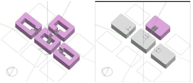
(21) Table 6. Number of buildings, built-up area (m2) and built-up area (%) per building type Building type MFT(≤4) UB1. UB2. MFT(>4). Construction period. No.. m. 1 (Before 1940). 2. 2 (1940-1959). 2. SFT(≤4). %. No.. m. 376. 1.05%. -. 7. 1,885. 5.27%. 3 (1960-1979). 7. 2,326. 4 (1980-2006). 4. 1,992. 5 (2007-2013). 1. 1 (Before 1940). 2. 2. %. No.. m. %. -. -. 14. 1,442. 3.92%. -. -. -. 12. 1,388. 3.77%. 6.51%. 34. 53,315. 23.89%. 6. 1,221. 3.32%. 5.57%. 20. 53,119. 23.80%. 3. 459. 1.25%. 426. 1.19%. 7. 9,694. 4.34%. 1. 231. 0.63%. 21. 4,419. 12.36%. -. -. -. 131. 15,954. 43.36%. 2 (1940-1959). 30. 6,724. 18.81%. 1. 146. 0.07%. 58. 7,661. 20.82%. 3 (1960-1979). 27. 8,656. 24.21%. 54. 60,797. 27.24%. 25. 3,796. 10.32%. 4 (1980-2006). 13. 7,972. 22.30%. 35. 39,865. 17.86%. 19. 3,435. 9.34%. 5 (2007-2013). 3. 979. 2.74%. 5. 6,245. 2.80%. 7. 1,206. 3.28%. 3.2. Stage II: energy performance assessment The energy demand for heating (EDh) and cooling (EDc) and discomfort hours for heating (DHh) and cooling (DHc) were taken as the reference indicators to assess the passive energy performance of the residential building stock in this study. In all, 240 dynamic energy simulations were run by combining the values of the five covariates (Figure 6) with the EnergyPlus software. One set of four values, which corresponded to the response variables, was obtained for all 240 hypotheses.. Figure 6. Simulations set-up scheme for determining EDc, EDh, DHc and DHh Figure 7 shows how the building was integrated into the urban layout to run simulations and presents, by way of example, building class MFT(≤4), situated in UB1 with H/W2.4, and building class MFT(>4) , situated in UB2 with H/W1.2, both of which are examples for the four solar orientations. As noted, the effect of the urban environment constraints is robustly considered. All the 240 hypotheses were created in separate files by combining geometric variables (UB, H/W, S/V), solar orientation (O) and, finally, the envelope solutions (Y) per construction period.. 21.

(22) Figure 7. Configuration layout in DesignBuilder for building class MFT(≤4) in UB1 and H/W2.4 (left) and building class MFT(>4) in UB2 and H/W1.2 (right) The input parameters for running simulations, such as occupancy, temperatures, internal gains, solar gains and domestic hot water (DHW) demand are presented in Table 7. The occupancy pattern was based on Spanish Building Code standards (CTE, 2013) according to density and schedule patterns. Similarly, the other parameters corresponded to official values for the operational loads established by CTE for residential buildings and for the specific climatic zone where the study was carried out. For the results obtained, heating season was considered to run from 1 October to 31 May, and the cooling season operated from 1 June to 30 September.. 22.

(23) Table 7. Boundary conditions set for the DesignBuilder software simulations Parameter (unit) Occupancy 2 Density (person/m ) Schedule pattern. Value. Metabolic rate (W/person) Clothing (clo) winter/summer. 0.03 Weekdays: 7:00-15:00h [25%]; 15:00-23:00h [50%]; 23:007:00h [100%] Weekends 0:00-24:00h [100%] 117.2 1/0.5. Temperatures (ºC) Heating set point Cooling set point Natural ventilation set point. 20 25 24. Internal gains 2 Internal loads (W/m ) 2 Lighting (W/m – 100 lux) 2 Miscellaneous gains (W/m ). 8.8 4.4 4.4. Solar gains Shading calculations include all surrounding buildings Calculations include modelling reflections and shading of ground reflected solar. Domestic hot water demand 2 DHW demand (l/m day). 0.84. 3.3. Stage III: statistical modelling The statistical inference based on INLA was conducted as described in Braulio-Gonzalo et al. (2016). Analyses were carried out with the R freeware statistical package (version 3.1) (R Development Core Team, 2011) and the R-INLA package (INLA, 2016) , developed by Rue and Martino (2007), and subsequently improved in Rue and Martino (2009). By combining all the covariates, 64 models were obtained. Once the battery of competing equations was obtained, we compared them by a Bayesian model comparison method (Pettit et al., 1990; Spiegelhalter et al., 2002) and selected the four best fitting equations to estimate the response variables, which are presented in Table 8. The set of four mathematical equations enabled the values for the response variables to be predicted in each single individual building of an urban area under study.. 23.

(24) Table 8. Prediction equations for response variables (Braulio-Gonzalo et al., 2016) Response. Prediction equation. variable EDc EDh DHc DHh. EDc  2.6480  0.3336  Y    6.5815  SV   0.0013  O  0.4637  HW   0.4372  UB . EDh  46.8932   17.6330  Y   118.4408  SV    0.0505  O  19.8277  HW   14.5047  UB . DH c  6.9152   2.1639  Y   13.6464  SV    0.0015  O  0.8659  HW   0.9760  UB  DH h  44.5077   0.9679  Y   12.5778  SV    0.004  O  0.8951  HW   0.9202  UB . Each single covariate considered herein was significant and contributed, to a greater or lesser extent, to improve the prediction models by thus reducing associated errors. This meant that the accuracy of the results increased by considering the whole set of covariates and not independently. 3.4. Stage IV: stock aggregation In the latest methodology stage, the results of assessing individual buildings were aggregated to extrapolate the conclusions on an urban scale. GIS technology combines geo-referenced information with cartography, which allows digital maps of urban areas to be developed to identify certain specific aspects of the built environment by a graphical interface. In this study, the cadastral data of the neighbourhood under study was processed by gvSIG software. For each cadastral plot, covariates were defined into the integrated attribute tables so that the application of the four equations to estimate the response variables was possible. As a result, energy demand and discomfort hours were determined for the entire neighbourhood building stock. In order to plot the results obtained on a GIS map, energy demand and discomfort hours were classified in an energy rating scale. For energy demand, this proposed classification was based on the energy class indicators for the existing buildings used in Spain. The scale was established from indicator A to G. As the values for EDc concentrated in class A and those for EDh in G, this study proposed an extended classification that broke down A and G into four additional indicators (A1, A2, A3, A4 and G1, G2, G3, G4) in order to accurately classify energy performance. Discomfort hours indicator is presented from classes A to F within ranges of 1,000 hours/year. Both indicators are shown in Table 9.. 24.

(25) Table 9. Class indicators for response variables ED and DH 2. 2. Energy class EDc (kWh/m •year) EDh (kWh/m •year) A1* EDc < 0.7 EDh < 4.7 A2* 0.7 ≤ EDc < 1.5 A3* 1.5 ≤ EDc < 3 A4* 3 ≤ EDc < 4.7 B 4.7 ≤ EDc < 7.6 4.7 ≤ EDh < 10.9 C 7.6 ≤ EDc < 11.7 10.9 ≤ EDh < 19.6 D 11.7≤ EDc < 18 19.6 ≤ EDh < 32.8 E 18 ≤ EDc < 22.3 32.8 ≤ EDh < 64.5 F 22.3 ≤ EDc < 27.4 64.5 ≤ EDh < 70.3 G1* 27.4 ≤ EDc 70.3 ≤ EDh < 102.3 G2* 102.3 ≤ EDh < 134.3 G3* 134.3 ≤ EDh < 166.9 G4* 166.9 ≤ EDh *The Spanish classification considers from A to G. A1, A2, A3, A4 and classes G1, G2, G3, G4 were proposed for this study.. DH class A B C D E F. DH (h/year) DH < 1,000 1,000 ≤ DH < 2,000 2,000 ≤ DH < 3,000 3,000 ≤ DH < 4,000 4,000 ≤ DH < 5,000 5,000 ≤ DH. The results of implementing the methodology into the neighbourhood under study were graphically represented on urban energy maps. Figures 8 and 9 show energy demand for cooling and heating, respectively, while Figures 10 and 11 show discomfort hours for cooling and heating, respectively.. Figure 8. Energy map: cooling energy demand of the buildings in the neighbourhood. 25.

(26) Figure 9. Energy map: heating energy demand of the buildings in the neighbourhood. Figure 10. Energy map: cooling discomfort hours of the buildings in the neighbourhood. 26.

(27) Figure 11. Energy map: heating discomfort hours of the buildings in the neighbourhood Plotting the results on urban energy maps channelled the identification of the interesting relationships among different aspects. In Figure 8, EDc was lower in the residential urban blocks that corresponded to type UB2, rather than UB1. This was due to the proximity between the inner façades in UB2, which entailed poor solar access and, consequently, lower cooling loads in the indoor building environment. Similar findings were obtained for heating energy demand with the urban block type (Figure 9). Those buildings with a higher EDh were placed mostly in UB2, where fewer solar access opportunities in winter led to increased heating loads. 4. Analysis of covariates influence When defining a methodology to predict the energy performance of residential stocks, the challenge was to find a limited number of covariates on both the building and urban scales that affected the response variables in relation to passive energy performance. We analysed the results obtained from simulations for each single covariate separately, which allowed us to draw some findings that helped understand the effect on the response variables (EDc, EDh, DHc and DHh). Figure 12 shows the results obtained for the response variables per covariate. Statistical analysis concluded that the five covariates are significant, ranked according to their level of significance as follows: S/V, Y, H/W, UB and O. 27.

(28) Urban block (UB). Height-width street ratio (H/W). Shape factor (S/V). 28.

(29) Year of construction (Y). Orientation (O). Figure 12. Response variables results (EDc, EDh, DHc, DHh) for covariates (UB, H/W, S/V, Y, O). 29.

(30) Regarding the shape factor (S/V), EDc displayed a clearly decreasing trend and came closer to 0 when the S/V was higher (less compact buildings), but this trend reversed for EDh, where heating energy demand diminished for lower S/V values, which implies more compactness. Discomfort hours were higher for less compact buildings for both heating and cooling. Thus we can conclude that more compact buildings are more energy-efficient in heating loads terms, and also contribute to achieve better levels of thermal comfort inside buildings. For year of construction (Y), the average heating energy demand for building types MFT(>4), MFT(≤4) and SFT(≤4) was represented in the five time periods. The trend was the same in the three buildings over time. The greatest energy demand lay in the buildings built before 1940 because of the poorer construction techniques employed then. In 1940-1959 a decrease in energy demand was denoted as one-layer load walls were replaced with double-layer walls with an air chamber, so the U-values lowered. In 1960-1979 the swift population growth in cities led to a rapid construction process with worse building features, especially roofs as the previous air chamber was replaced with a light concrete layer. After the oil crisis in the 1970s, thermal insulation requirements came into force (NBE-CT-79, 1979) and the buildings built in 1980-2006 demanded much less energy. Finally, when CTE came into force, and given the consequent tightening of insulation requirements, buildings demanded slightly less energy. Thus heating energy demand notably reduced as construction techniques improved over the years, and also as thermal insulation material was introduced into the building’s envelope. However, the implementation of CTE (2006) did not involve more thermal requirements compared to NBE-CT-79 (1979), as reflected in Table 5, where the drop in heating energy demand is almost negligible. For street H/W ratio, EDc decreased for H/W2.4 (narrow streets), due to the lower solar gains in the buildings’ façades. However, DHc and DHh notably increased for H/W2.4, which denote that higher H/W ratios implied worse thermal comfort conditions for buildings occupants. Therefore, H/W shall be such that buildings’ façade shall receive during the winter solstice (solar elevation of 26.61° in the latitude of Castellón de la Plana), at least, two hours of sunlight (Higueras, 2006). This implies designing a H/W ratio of 0.50. Regarding the covariate urban block (UB), we noted that EDc decreased for UB2, where the inexistence of a block courtyard impeded solar irradiation, as it also did with solar gains inside the building, especially in summer. For EDh, we were unable to find a significant difference between both block kinds. However as for discomfort hours, we observed that both DHc and DHh increased in UB2 as there were fewer possibilities of solar gains and natural ventilation, so buildings situated in UB1 present much better passive energy performance. 30.

(31) In relation to orientation (O), we note that the lowest EDc values went to north-oriented buildings, followed by those oriented to the south, east and west (the highest values). Little variation among orientations is noted in EDh, which demonstrates that urban morphology and the surrounding built environment can strongly influence on the passive energy performance of buildings. Considering the above, a set of urban and building design strategies can be drawn to minimise energy demand and improve thermal comfort conditions, which are presented in Table 10. These can be considered when designing new urban planning developments. Table 10. Strategies related to covariates to improve passive energy performance of residential stocks Covariate S/V Y H/W UB O. Strategy Reduce the building shape factor (S/V) to values close to 0.26 Reduce U-values and ψ of constructive elements and thermal bridges Establish H/W ratio of 0.50, in order to ensure solar gains in building’s façades even in winter period Design urban blocks with big internal courtyards (UB1 typology) that allows, at least, two different orientations in every single building that compound the block Prioritise South orientation of buildings’ façades, which implies designing rectangular blocks with the long side south-oriented. Additional simulations carried out demonstrated that an orientation of 18° towards SE was the optimum to achieve lower values for EDc and EDh, as shown in Supplementary Information 2. 5. Validation of the methodology According to Table 10, a set of urban design strategies can be considered to draw a new planning proposal. The comparison of passive energy performance results between the current neighbourhood and the new planning proposal leads to obtain the energy demand savings that can be achieved. Limitations imposed by the City Urban Plan were also considered to design a new planning development with the same land area of 17.6 hectares as the current neighbourhood, as shown in Figure 13, in order both cases can be compared.. Figure 13. Current neighbourhood planning (left) and new planning proposal (right) with 17.6 hectares 31.

(32) The results of assessing both scenarios reveal that a reduction of 57.12% in global energy demand, both heating and cooling, can be achieved by implementing the new urban planning design, which means considering only geometrical aspects. Table 11 shows the results obtained. Although EDc presents a notable increase with the new planning in relation to the current scenario, the value of 1,073.88 MWh/year only represents 8.4% of the global energy demand (12,813.20 MWh/year), so this increase compensates the higher reduction in EDh (60.01%), which is responsible for the most of the global energy demand in the neighbourhood. Table 11. Variation of energy demand in two different urban planning (17.6 hectares). 2. Buildings built-up area (m ) EDc (MWh/year) EDh (MWh/ year) EDG* (MWh/ year) *EDG: Global energy demand. Current neighbourhood 313,301.00 523.53 29,354.89 29,878.42. New planning proposal 275,849.4 1,073.88 11,739.32 12,813.20. Variation (%) -11.95% 205.13% -60.01% -57.12%. This comparison shows that the methodology results enabled informed variations to be made in the covariates with significant energy savings. Thus the application of the methodology proved that taking into account the outlined strategies for designing new urban developments in the city had positive implications on the local level, as involved important energy demand reductions by only considering passive geometrical design aspects on both the building and city scales. 6. Discussion and conclusions A bottom-up-based methodology was developed to assess the energy performance and indoor thermal comfort of residential stocks on an urban scale. The proposed methodology enables the quantification of two main aspects that act as environmental performance indicators: energy demand (for heating and cooling) and discomfort hours (for heating and cooling) of the buildings that compound a stock according to both building and urban intrinsic parameters. Thus not only the building as an individual item is approached, but also the building in the urban context it is placed in. Statistical modelling showed that energy performance and indoor comfort strongly correlate with building and urban parameters. In this study, the number of values of covariates corresponded to the intrinsic urban design morphology of the neighbourhood under study. Thus three building typologies, five temporal periods, two street H/W ratios, two urban blocks and four solar orientations were considered. Although a local sensitivity analysis has been conducted in several literature reports (Demanuele et al., 2010; Kavgic et al., 2013; Lam and Hui, 1996; Rasouli et al., 2013), this study applied a global. 32.

(33) sensitivity method through INLA to analyse the interactions among covariates and to explain how much variations of the response variables are accounted by covariates. A sensitivity analysis was conducted by varying the value adopted by these covariates and by analysing the effect of these changes on the response variables. As a result, we found that the building typology (denoted by S/V) and the building envelope assemblies U-values (denoted by Y) were the most significant covariates. Almost with the same significance as Y, the street H/W ratio strongly affected the response variables since it conditioned the solar access possibilities. UB and O were the least influential covariates. Consequently, urban layout should be integrated when analysing a building or a set of buildings in energy terms and when developing stock aggregation models. The complex prediction method employed in this work allows the accurate assessment of every single building that compounds the urban area under study, taking into account the specific urban parameters related to the building. This avoids making generalisations, emerged when steady energy use indicators are associated to a building stock by only considering the building class, which usually arises when conducting a simple stock aggregation process. In addition, knowing the key covariates that affect the energy and comfort performance obtained from the sensitivity analysis can facilitate policymakers the application of urban design strategies. As Kavgic et al. (2013), Tian (2013) and Hemsath and Alagheband Bandhosseini (2015) concluded, sensitivity analyses play an important role in building energy analyses to support model predictions. The integration of GIS helps create an urban geo-referenced database that contains valuable information and facilitates the characterisation of the residential building stock. It also enables the study results to be plotted on urban energy maps, which is considered an important point to help stakeholders make informed and transparent decisions. It enables users to analyse critical issues through a friendly visual interface, while also informs citizens about the energy performance of their dwellings. So the methodology is a transparent instrument for both local authorities and citizens. Urban energy maps can also be continuously improved by adding any other kind of information on the urban or building scale, such as technological or socio-economic aspects, as Dall’O' et al. (2013) proposed in a multi-criteria model to support public administration decision making on sustainable energy action plans. By comparing the reviewed models with the proposed methodology, it is worth pointing out that any of them met the six requirements established all together. As seen in Table 12, all models considered at least one requirement and, although Fonseca and Schlueter (2015) integrated the six, urban covariates are not considered in their model to energy assess the building stock. The methodology presented here combined different technologies that enriched the accuracy of the work. 33.

(34) Table 12. Requirements met by reviewed bottom-up models. • • • •. • •. • • •. • • • • •. • • •. • • • • • • • •. • •. • • •. • • •. • • • • • • • • • • • • • •. • • • • • • • • • • • • • • • • • • • • • • • • •. D. E. F. Statistical modelling. GIS environment. Y. S/V. O. H/W. UB. C. DH. ED. Context adaptive. Model CREEM (Farahbakhsh et al., 1998) Huang and Berkeley (2000) Ren et al. (2012) Snäkin (2000) BREEHOMES (Shorrock and Dunster, 1997) Johnston et al. (2005) UKDCM (Boardman, 2007) DECarb (Natarajan and Levermore, 2007) EEP (Jones et al., 2007) CDEM (Firth et al., 2010) DECM (Cheng and Steemers, 2011) VerbCO2M (Hens et al., 2001) TABULA (Dascalaki et al., 2011) Dall’O’ et al. (2012) Caputo et al. (2013) Ascione et al. (2013) SLABE (Mauro et al., 2015) Penna et al. (2015) TIMES (Gouveia et al., 2012) TABULA (Florio and Teissier, 2015) Fonseca and Schlueter (2015) QuBEC (Aksoezen et al., 2015) ECCABS (Mata et al., 2013) McKenna et al. (2013) TABULA (Instituto Valenciano de la Edificación, 2014) Camargo-Ramirez (2012) Laubinger (2015). B. Dynamic simulation. Methodology requirements A. • • •. • •. • • •. • • • •. • •. •. • •. •. •. • •. •. • •. The comparison between two different urban morphologies demonstrated that when implementing informed design strategies in new urban developments, notable energy demand savings can be achieved, by only considering passive aspects both on the building and urban scales based on geometrical constraints. The methodology is conceived as a generic multi-staged methodology that can be replicated in the other neighbourhoods of the analysed city, or in any other city, by implementing the steps described herein. It has also been defined as a lively method that can be continuously updated with the addition of new variables or covariates in order to investigate other aspects and their relationship with building energy performance. The results obtained herein and the proposed methodology can act as a basis for further research in this field to include a larger number of covariates, and to explore a more extensive casuistry.. 34.

(35) The model allows stakeholders involved in urban processes, such as architects, urban planners, engineers and local authorities, establishing environmental policies and programmes to promote sustainable urban development initiatives. In addition, the model can help local authorities identify vulnerable neighbourhoods in energy efficiency terms by comparing energy demand and thermal discomfort along urban blocks in a city, in order to set priority guidelines when building refurbishment processes and urban regeneration projects have to be conducted locally.. References Aksoezen, M., Daniel, M., Hassler, U., Kohler, N., 2015. Building age as an indicator for energy consumption. Energy Build. 87, 74–86. doi:10.1016/j.enbuild.2014.10.074 Ascione, F., De Masi, R.F., de Rossi, F., Fistola, R., Sasso, M., Vanoli, G.P., 2013. Analysis and diagnosis of the energy performance of buildings and districts: Methodology, validation and development of Urban Energy Maps. Cities 35, 270–283. doi:10.1016/j.cities.2013.04.012 Asociación gvSIG, 2014. gvSIG Desktop. Balaras, C.A., Gaglia, A.G., Georgopoulou, E., Mirasgedis, S., Sarafidis, Y., Lalas, D.P., 2007. European residential buildings and empirical assessment of the Hellenic building stock, energy consumption, emissions and potential energy savings. Build. Environ. 42, 1298–1314. doi:http://dx.doi.org/10.1016/j.buildenv.2005.11.001 Boardman, B., 2007. Examining the carbon agenda via the 40% House scenario. Build. Res. Inf. 35, 363–378. doi:10.1080/09613210701238276 Braulio-Gonzalo, M., Bovea, M.D., Ruá, M.J., 2015a. Sustainability on the urban scale: Proposal of a structure of indicators for the Spanish context. Environ. Impact Assess. Rev. 53, 16–30. doi:10.1016/j.eiar.2015.03.002 Braulio-Gonzalo, M., Juan, P., Bovea, M.D., Ruá, M.J., 2016. Modelling energy efficiency performance of residential building stocks based on Bayesian statistical inference. Environ. Model. Softw. 83, 198–211. doi:10.1016/j.envsoft.2016.05.018 Braulio-Gonzalo, M., Ruá Aguilar, M., Bovea Edo, M., 2015b. Characterisation of urban patterns at the neighbourhood scale as an energy parameter. Case study: Castellón de la Plana, in: Mercader Moyano, P. (Ed.), Proceedings of the II International and IV National Congress on Sustainable Construction and Eco-Efficient Solutions. University of Seville, Sevilla, pp. 1069– 1079. Camargo-Ramirez, L.E., 2012. A GIS-Based Method for Predicting Hourly Domestic Energy Need for Space Conditioning and Water Heating of Districts and Municipalities. Universität für Bodenkultur Wien. Capeluto, I.G., 2003. The influence of the urban environment on the availability of daylighting in office buildings in Israel. Build. Environ. 38, 745–752. doi:10.1016/S0360-1323(02)00238-X Caputo, P., Costa, G., Ferrari, S., 2013. A supporting method for defining energy strategies in the building sector at urban scale. Spec. Sect. Long Run Transitions to Sustain. Econ. Struct. Eur. Union Beyond 55, 261–270. doi:http://dx.doi.org/10.1016/j.enpol.2012.12.006 35.

(36) CEN, 2012. EN ISO 6946:2012 Building components and building elements - Thermal resistance and thermal transmittance - Calculation method. CEN, 2011a. EN ISO 673:2011 Glass in building. Determination of thermal transmittance (U value). Calculation method. CEN, 2011b. EN ISO 14683, Thermal bridges in building construction – Linear thermal transmittance – Simplified methods and default values. Cheng, V., Steemers, K., 2011. Modelling domestic energy consumption at district scale: A tool to support national and local energy policies. Environ. Model. Softw. 26, 1186–1198. doi:10.1016/j.envsoft.2011.04.005 CTE, 2013. Orden FOM/1635/2013, de 10 de septiembre, por la que se actualiza el Documento Básico DB-HE Ahorro de Energía del Código Técnico de la Edificación, aprobado por Real Decreto 314/2006, de 17 de marzo. España. CTE, 2006. Real Decreto 314/2006, de 17 de marzo, por el que se aprueba el Código Técnico de la Edificación. España. Dall’O’, G., Galante, A., Torri, M., 2012. A methodology for the energy performance classification of residential building stock on an urban scale. Energy Build. 48, 211–219. doi:10.1016/j.enbuild.2012.01.034 Dall’O', G., Norese, M.F., Galante, A., Novello, C., 2013. A multi-criteria methodology to support public administration decision making concerning sustainable energy action plans. Energies 6, 4308–4330. doi:10.3390/en6084308 Dascalaki, E.G., Droutsa, K.G., Balaras, C.A., Kontoyiannidis, S., 2011. Building typologies as a tool for assessing the energy performance of residential buildings – A case study for the Hellenic building stock. Energy Build. 43, 3400–3409. doi:http://dx.doi.org/10.1016/j.enbuild.2011.09.002 De Jong, M., Yu, C., Chen, X., Wang, D., Weijnen, M., 2013. Developing robust organizational frameworks for Sino-foreign eco-cities: Comparing Sino-Dutch Shenzhen Low Carbon City with other initiatives. J. Clean. Prod. 57, 209–220. doi:10.1016/j.jclepro.2013.06.036 Demanuele, C., Tweddell, T., Davies, M., 2010. Bridging the gap between predicted and actual energy performance in schools, in: World Renewable Energy Congress XI. Abu Dhabi. DesignBuilder UK, 2015a. DesignBuilder help [WWW http://www.designbuilder.co.uk/helpv3.4/ (accessed 12.12.15).. Document].. URL. DesignBuilder UK, 2015b. DesignBuilder software. DGC, 2014. Dirección General del Catastro. Estiri, H., 2014. Building and household X-factors and energy consumption at the residential sector. Energy Econ. 43, 178–184. doi:10.1016/j.eneco.2014.02.013 Fabbri, K., Zuppiroli, M., Ambrogio, K., 2012. Heritage buildings and energy performance: Mapping with GIS tools. Energy Build. 48, 137–145. doi:10.1016/j.enbuild.2012.01.018 Farahbakhsh, H., Ugursal, V.I., Fung, A.S., 1998. A residential end-use energy consumption model for Canada. Int. J. Energy Res. 22, 1133–1143. doi:10.1002/(SICI)1099114X(19981025)22:13<1133::AID-ER434>3.0.CO;2-E 36.

(37) Firth, S.K., Lomas, K.J., Wright, a. J., 2010. Targeting household energy-efficiency measures using sensitivity analysis. Build. Res. Inf. 38, 25–41. doi:10.1080/09613210903236706 Florio, P., Teissier, O., 2015. Estimation of the Energy Performance Certificate of a housing stock characterised via qualitative variables through a typology-based approach model: A fuel poverty evaluation tool. Energy Build. 89, 39–48. doi:10.1016/j.enbuild.2014.12.024 Fonseca, J.A., Schlueter, A., 2015. Integrated model for characterization of spatiotemporal building energy consumption patterns in neighborhoods and city districts. Appl. Energy 142, 247–265. doi:10.1016/j.apenergy.2014.12.068 Futcher, J.A., Mills, G., 2013. The role of urban form as an energy management parameter. Energy Policy 53, 218–228. doi:10.1016/j.enpol.2012.10.080 Garrido-Soriano, N., Rosas-Casals, M., Ivancic, A., Álvarez-del Castillo, M.D., 2012. Potential energy savings and economic impact of residential buildings under national and regional efficiency scenarios. A Catalan case study. Energy Build. 49, 119–125. doi:http://dx.doi.org/10.1016/j.enbuild.2012.01.030 Gouveia, J.P., Fortes, P., Seixas, J., 2012. Projections of energy services demand for residential buildings: Insights from a bottom-up methodology. Energy 47, 430–442. doi:10.1016/j.energy.2012.09.042 Granadeiro, V., Correia, J.R., Leal, V.M.S., Duarte, J.P., 2013. Envelope-related energy demand: A design indicator of energy performance for residential buildings in early design stages. Energy Build. 61, 215–223. doi:10.1016/j.enbuild.2013.02.018 Hemsath, T.L., Alagheband Bandhosseini, K., 2015. Sensitivity analysis evaluating basic building geometry’s effect on energy use. Renew. Energy 76, 526–538. doi:10.1016/j.renene.2014.11.044 Hens, H., Verbeeck, G., Verdonck, B., 2001. Impact of energy efficiency measures on the CO2 emissions in the residential sector, a large scale analysis. Energy Build. 33, 275–281. Higueras, E., 2006. Urbanismo bioclimático ISBN: 978-84-252-2071-5. Gustavo Gili, Barcelona. Huang, Y.J., Berkeley, L., 2000. A Bottom-Up Engineering Estimate of the Aggregate Heating and Cooling Loads of the Entire US Building Stock Prototypical Residential Buildings, in: Proceedings of the 2000 ACEEE Summer Study on Energy Efficiency in Buildings. Pacific Grove, pp. 135–148. INE, 2015. Spanish Statistical Office [WWW Document]. URL http://www.ine.es/ INLA, 2016. R-INLA project [WWW Document]. URL http://www.r-inla.org/ (accessed 9.15.15). Instituto Valenciano de la Edificación, 2014. TABULA. Catálogo de tipología edificatoria residencial en España. Valencia. Johnston, D., Lowe, R., Bell, M., 2005. An exploration of the technical feasibility of achieving CO2 emission reductions in excess of 60% within the UK housing stock by the year 2050. Energy Policy 33, 1643–1659. doi:10.1016/j.enpol.2004.02.003 Jones, P., Patterson, J., Lannon, S., 2007. Modelling the built environment at an urban scale—Energy and health impacts in relation to housing. Landsc. Urban Plan. 83, 39–49. doi:10.1016/j.landurbplan.2007.05.015 Kavgic, M., Mavrogianni, a., Mumovic, D., Summerfield, a., Stevanovic, Z., Djurovic-Petrovic, M., 37.

(38) 2010. A review of bottom-up building stock models for energy consumption in the residential sector. Build. Environ. 45, 1683–1697. doi:10.1016/j.buildenv.2010.01.021 Kavgic, M., Mumovic, D., Summerfield, A., Stevanovic, Z., Ecim-Djuric, O., 2013. Uncertainty and modeling energy consumption: Sensitivity analysis for a city-scale domestic energy model. Energy Build. 60, 1–11. doi:10.1016/j.enbuild.2013.01.005 Košir, M., Capeluto, I.G., Krainer, A., Kristl, Ž., 2014. Solar potential in existing urban layouts—Critical overview of the existing building stock in Slovenian context. Energy Policy 69, 443–456. doi:10.1016/j.enpol.2014.01.045 Lam, J.C., Hui, S.C.M., 1996. Sensitivity analysis of energy performance of office buildings. Build. Environ. 31, 27–39. doi:10.1016/0360-1323(95)00031-3 Laubinger, F., 2015. A bottom-up analysis of household energy consumption in Amsterdam. Resolving policy barriers in the residential building sector. Amsterdam University College. Martins, T.A.L., Adolphe, L., Bastos, L.E.G., 2014. From solar constraints to urban design opportunities: Optimization of built form typologies in a Brazilian tropical city. Energy Build. 76, 43–56. doi:10.1016/j.enbuild.2014.02.056 Mata, É., Kalagasidis, A.S., Johnsson, F., 2013. A modelling strategy for energy, carbon, and cost assessments of building stocks. Energy Build. 56, 100–108. doi:10.1016/j.enbuild.2012.09.037 Mauro, G.M., Hamdy, M., Vanoli, G.P., Bianco, N., Hensen, J.L.M., 2015. A new methodology for investigating the cost-optimality of energy retrofitting a building category. Energy Build. 107, 456–478. doi:10.1016/j.enbuild.2015.08.044 Mavrogianni, A., Wilkinson, P., Davies, M., Biddulph, P., Oikonomou, E., 2012. Building characteristics as determinants of propensity to high indoor summer temperatures in London dwellings. Build. Environ. 55, 117–130. doi:10.1016/j.buildenv.2011.12.003 McKenna, R., Merkel, E., Fehrenbach, D., Mehne, S., Fichtner, W., 2013. Energy efficiency in the German residential sector: A bottom-up building-stock-model-based analysis in the context of energy-political targets. Build. Environ. 62, 77–88. doi:10.1016/j.buildenv.2013.01.002 Moffatt, S., 2001. Methods for the evaluation of the environmental performance of building stock. Editorial review by Illari Aho, Findland. Natarajan, S., Levermore, G.J., 2007. Predicting future UK housing stock and carbon emissions. Energy Policy 35, 5719–5727. doi:10.1016/j.enpol.2007.05.034 NBE-CT-79, 1979. Real Decreto. Norma Básica de la Edificación sobre condiciones térmicas en los edificios. España. Oke, T.R., 1988. Street design and urban canopy layer climate. Energy Build. 11, 103–113. doi:10.1016/0378-7788(88)90026-6 Penna, P., Prada, A., Cappelletti, F., Gasparella, A., 2015. Multi-objectives optimization of Energy Saving Measures in existing buildings. 49th AICARR Int. Conf. - Hist. Exist. Build. Des. retrofit 95, 57–69. doi:10.1016/j.enbuild.2014.11.003 Pettit, A.L.I., Journal, S., Statistical, R., Series, S., 1990. The conditional predictive ordinate for the normal distribution 52, 175–184. R Development Core Team, 2011. R: A Language and Environment for Statistical Computing. 38.

(39) Rasouli, M., Ge, G., Simonson, C.J., Besant, R.W., 2013. Uncertainties in energy and economic performance of HVAC systems and energy recovery ventilators due to uncertainties in building and HVAC parameters. pp. 732–742. doi:10.1016/j.applthermaleng.2012.08.021 Ren, Z., Paevere, P., McNamara, C., 2012. A local-community-level, physically-based model of enduse energy consumption by Australian housing stock. Energy Policy 49, 586–596. Rue, H., Martino, S., 2009. Approximate Bayesian inference for latent Gaussian models by using integrated nested Laplace approximations. J. R. Stat. Soc. 319–392. Rue, H., Martino, S., 2007. Approximate Bayesian inference for hierarchical Gaussian Markov random field models. J. Stat. Plan. Inference 137, 3177–3192. doi:10.1016/j.jspi.2006.07.016 Rue, H., Martino, S., Chopin, N., 2009. Approximate Bayesian inference for latent Gaussian models by using integrated nested Laplace approximations. J. R. Stat. Soc. 72, 319–392. Salat, S., 2009. Energy loads, CO2 emissions and building stocks: morphologies, Typologies, Energy Systems and Behaviour. Build. Res. Inf. 37, 598–609. doi:10.1080/09613210903162126 Shorrock, L., Dunster, J., 1997. The physically-based model BREHOMES and its use in deriving scenarios for the energy use and carbon dioxide emissions of the UK housing stock. Energy Policy 25, 1027–1037. doi:10.1016/S0301-4215(97)00130-4 Singh, M., Attia, S., Mahapatra, S., Teller, J., 2016. Assessment of thermal comfort in existing pre1945 residential building stock. Energy 98, 122–134. doi:10.1016/j.energy.2016.01.030 Snäkin, J.-P.A., 2000. An engineering model for heating energy and emission assessment The case of North Karelia, Finland. Appl. Energy 67, 353–381. Spiegelhalter, D.J., Best, N.G., Carlin, B.P., 2002. Bayesian measures of model complexity and fit 583– 639. Swan, L.G., Ugursal, V.I., 2009. Modeling of end-use energy consumption in the residential sector: A review of modeling techniques. Renew. Sustain. Energy Rev. 13, 1819–1835. doi:10.1016/j.rser.2008.09.033 Terés-Zubiaga, J., Martín, K., Erkoreka, a., Sala, J.M., 2013. Field assessment of thermal behaviour of social housing apartments in Bilbao, Northern Spain. Energy Build. 67, 118–135. doi:10.1016/j.enbuild.2013.07.061 Theodoridou, I., Karteris, M., Mallinis, G., Papadopoulos, A.M., Hegger, M., 2012. Assessment of retrofitting measures and solar systems’ potential in urban areas using Geographical Information Systems: Application to a Mediterranean city. Renew. Sustain. Energy Rev. 16, 6239–6261. doi:http://dx.doi.org/10.1016/j.rser.2012.03.075 Theodoridou, I., Papadopoulos, A.M., Hegger, M., 2011a. A typological classification of the Greek residential building stock. Energy Build. 43, 2779–2787. doi:http://dx.doi.org/10.1016/j.enbuild.2011.06.036 Theodoridou, I., Papadopoulos, A.M., Hegger, M., 2011b. Statistical analysis of the Greek residential building stock. Energy Build. 43, 2422–2428. doi:10.1016/j.enbuild.2011.05.034 Tian, W., 2013. A review of sensitivity analysis methods in building energy analysis. Renew. Sustain. Energy Rev. 20, 411–419. doi:10.1016/j.rser.2012.12.014 U.S. Department of Energy, 2013. Energy Plus software. 39.

(40) Uihlein, A., Eder, P., 2010. Policy options towards an energy efficient residential building stock in the EU-27. Energy Build. 42, 791–798. doi:10.1016/j.enbuild.2009.11.016 Yezioro, A., Capeluto, I.G., Shaviv, E., 2006. Design guidelines for appropriate insolation of urban squares. Renew. Energy 31, 1011–1023. doi:10.1016/j.renene.2005.05.015 Yin, Y., Rader Olsson, A., Håkansson, M., 2015. The role of local governance and environmental policy integration in Swedish and Chinese eco-city development. J. Clean. Prod. 1–9. doi:10.1016/j.jclepro.2015.10.087. 40.

(41)