Forecasting Models Selection Mechanism for Supply Chain Demand Estimation

(1)

Procedia Computer Science 55 ( 2015 ) 1060 – 1068

Peer-review under responsibility of the Organizing Committee of ITQM 2015 doi: 10.1016/j.procs.2015.07.068

ScienceDirect

Information Technology and Quantitative Management (ITQM 2015)

Forecasting Models Selection Mechanism for Supply Chain

Demand Estimation

Juan Pedro Sepúlveda-Rojas

a

_{*, Felipe Rojas}

b

_{, Héctor Valdés-González}

b

_{, Mario San}

Martín

b

Department of Industrial Engineering, University of Santiago of Chile, Avenida Ecuador 3769, Santiago, Chile Facultad de Ingeniería, Universidad Andres Bello, Sazié 2325, Santiago, Chile

Abstract

The aim of this work is to present a selection mechanism of forecast models to contribute to demand estimation in a supply chain. At present, to estimate a product future demand, several forecast models based on historical information -quantitative and qualitative- are used. When companies face this situation, they select a group of forecast models (usually based on a visual basis of the time series), then estimate, and with the forecast error measurement criteria decide which the best method is. But they always have to estimate over all the selected forecast models. Based on that, this paper introduces an alternative methodology to estimate the best-forecast model without the need to estimate all the forecast models or complement with another technique (visual). To do so, the main theoretical fundaments associated to this new methodology are addressed, and then the methodology itself is presented in order to be applied in two real cases of Chilean companies to finally conclude the results of the described mechanism.

Selection and/or peer-review under responsibility of the organizers of ITQM 2015

Keywords: Time Series, Autocorrelation Coefficient, Forecasting.

1. Introduction

Due to the existence of unknown and uncontrollable future sceneries, several quantitative and qualitative forecasting techniques appear in order to approximately visualize future events, techniques that become relevant in decision making for companies and organizations. These techniques have become complex systems capable to transform simple data in understandable and accessible information for the company, tools focused in the administration and generation of knowledge through data analysis, strategically contributing to the logistics of organizations.

* Corresponding author. Tel.: +56-2-2718-4114; fax: +56-2-2779-9723. E-mail address:[email protected].

(2)

It is well know that an important business cost is related to the inventories, such as raw material inventory, work in progress and final product inventory. [1] argue that accurate forecasting can reduce or eliminate inventory costs.

[2] argue that, in a sense, inventory exists to be a buffer for inexact forecasts, thus, the more accurate forecasts are, less inventory needs to be carry out, with all the cost savings this brings.

Moreover, [3] explain that demand forecast drives supply chain and demand planner drives forecast process, while [4] argue that future demand forecast is the basis of all strategic decisions and planning in a supply chain. Thus, the role played by demand forecasts in companies is fundamental through supply chain to reduce inventory costs, wait time, supply costs, etc.

In the current context, this article attempts to establish an alternative mechanism to select a forecast method to complement the existing methods and apply it to a real case, and finally make conclusions and generate discussion.

This article is organized as follows. The literature review about this subject is presented in section 2. In section 3 the selection mechanism is formally presented. In sections 4 and 5 the applied cases are analyzed. Finally the article is concluded in section 6.

2. Literature review

[5] argue that there are literature that incorporate the treatment of random demand to inventory systems and use probability distributions to make forecast, while [6] say that a revision of forecast errors over time may indicate if the forecasting technique being used match with demand. [7] explain that mean error (ME) and mean percentage error (MPE) present advantages to measure the bias in a forecast. Negative ME or MPE suggest the forecast model overestimate the forecasting, while positive ME or MPE suggests previsions are to low in general. According to these authors, a highlighted criterion is MAPE.

[7] give a reference framework that helps to determine when to use each forecast method once there is a general comprehension of several forecasting techniques. They affirm that there are numerous characteristics in a forecasting situation that may be considered when selecting an adequate method.

The reference framework provided by [7] focuses the attention in three main areas: data, time and human resources. It considers type and amount of data, as well as any patter among them (trend, cycle, and seasonality). The second one focuses on time horizon. And human resources consider the technical knowledge about forecasting techniques. [8] give a summary table to select forecast methods and suggest techniques (including visual inspection of time series) to be used with determined data patterns. That table is focused on time series forecast models specifying for which time horizon and data pattern are useful.

[9] argues that Data Mining tools may answer questions that usually take so much time to find. Says that data mining is actually an iterative process to find patterns and tendencies in data, through automatic, manual or semi automatic methods. In addition, the author explains that data mining tools explore databases to find hidden patterns to predict future tendencies and behavior of new information. In this case, Data Mining tools not necessary need a visual inspection of time series, however the used techniques are unknown for the users. It looks like a black box for the users. A difference with this article is that with a simple analysis is possible to know the pattern of time series and hence, make a more accurate selection of the forecast technique.

(3)

3. Selection mechanism of forecasting models for demand estimation

This mechanism developed a five steps sequence to make the forecast. Two of them define the product or service and gather data. Previously mentioned steps correspond to a basic sequence to forecast, however, this work suggests a different third step (analyze data pattern).

3.1. Analyze data patterns

It consists of a previous data analysis to visualize the time series characteristics; to accurately and precisely select the best forecast techniques. Therefore, to avoid problems selecting the best method, a tool to characterize and determine the time series pattern is needed.

Although it is recommended, as a prior an intuitive analysis, a graphic representation of time series evolution is needed to analyze its behavior. However it is not always possible to correctly conclude about patterns, so, a more sophisticated tool is needed in this case.

The tool that this article propose is to analyze data pattern with an autocorrelation analysis, which aim is to determine time series relationship, when it has a time lag of one or more periods, which formula is:

ݎ

௞

=

σ೙షೖ೟సభ(௫೟ି௫ҧ)(௫೟శೖି௫ҧ)

σ೙೟సభ(௫೟ି௫ҧ)మ (1)

Given a sequence of observations x1, x2,…, xn, n–1 contiguous observation pairs can be made (x1,x2),

(x2,x3),…, (xn-1,xn) and calculate the first order autocorrelation coefficient of this pairs. The first time lag

coefficient is called autocorrelation coefficient at lag 1, indicated as r1. Generally, when separating pairs for k

distance, k order autocorrelation coefficient can be calculated. According to [10], simple autocorrelation function (FAS) measure the correlation between time series separated a k period of time. The autocorrelation function is the set of autocorrelation coefficients of rk, from k=1 to a maximum that cannot exceed half of the

series observations. This limit is imposed by the impossibility to look for autocorrelations between values beyond the beginning (or end) of the time series.

[10] explains that, theoretically, the coefficient can take values between -1 and 1, moreover, [11] say that a positive autocorrelation close to 1 shows a stronger correlation between time series values with a lag of k time units. When the autocorrelation coefficient is negative and close to -1, data depends inversely.

[10] says that, in real life situations, rk could take values different from zero without correlation between

observed values in a k distance. To measure if that distance from zero is significant (existence of correlation), a contrast of statistical significance is done with a signification interval for rk about rk=0, with significant

coefficients if they are over the bands.

Significance interval for the correlation coefficient can be built with the standard error calculation. It can be calculated with the following mathematical expression:

ܵ_௥௞=ටଵାଶ σ೙షభ೔సభ௥೔మ

௡ (2)

[12] says that Bartlett in 1946 demonstrated that in the event of normality of stochastic processes, the delays of FAS have a roughly normal distribution with a mean of zero and typical deviation :

ට

ଵାଶ σ೙షభ೔సభ௥೔మ

(4)

Thus, significance interval for rk can be implicitly estimated with a standard normal value (z) of 1,96

deviations of Srk, which results in a probability of non-significance difference from zero of the simple

autocorrelation coefficient of 95% and a difference to zero associated to a probability of 5%. Significance bands, therefore, are established as (Srk) above and (Srk) under the central axis in 0. If the simple autocorrelation

coefficient value, for lag k, results outside the significant difference interval from zero, is related to a low probability to be caused by chance. Thus, if this happen, there are correlation between the observed variable values at a k lag, that is to say, to consider a coefficient as significantly different from zero, this must exceed the limits of the significance interval.

[8] and [6] say that t-statistics, associated to the correlation coefficient calculation, allows also judge about the significance of it. For rk, we estimate trklike rk/Srk. To significantly consider rkdifferent from zero, so tnere

is autocorrelation, the value of this statistical must be higher than 1,96 in absolute value.

To understand the autocorrelations behavior (r1,r2,….rk) there is a table or graphic called autocorrelogram,

that allows to identify previously mentioned patterns (r1,r2,….rk), it shows the coefficients as well as significant

difference bands from zero. Autocorrelogram is a useful tool to show autocorrelations for several time lags in a data series [8]. Table 1 shows possible behaviors of a time series can have and the t-statistics.

Table 1 Analysis of t-statistics associated with autocorrelation coefficient. Source: [8]

Possible scenarios t- statistics behavior

Significant Statistical (there is autocorrelation) |ݐ௥௞| > 1,96

Random Series All delays shows a |ݐ௥௞| < 1,96

Series with Trend Several of the first delays shows a |ݐ௥௞| < 1,96. All of them

decrease, after the first delay, gradually to zero when the increase of the number of periods.

Seasonal Series It shows a significant |ݐ௥௞|in the corresponding time lag (|ݐ௥௞|>

1,96), four on quarterly data or twelve on monthly data.

Stationary Series |ݐ௥௞|values suddenly decrease to zero (<1,96) after the second or

third period of time lag. That is, tr1, tr2and up to tr3could present

significant values, being all other statistics close to zero.

3.2. Selection of Forecasting Model

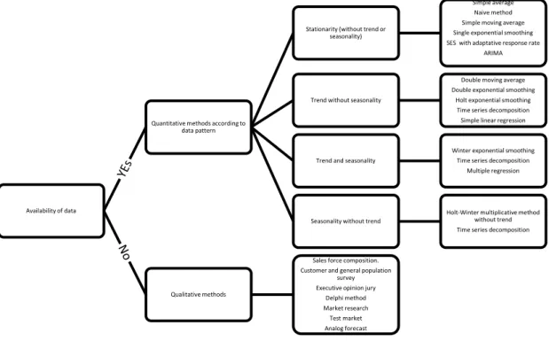
A decision tree of forecast methods (Fig 1) was developed to illustrate the selection of forecast method, it resumes what [7] and [8] proposed to select the best forecasting method, according to the series data pattern.

Forecast methods decision tree (Fig 1) helps to pre-select alternative methods to forecast future demand. Finally, to select the most adequate alternative proposed by the decision tree, a retrospective analysis of data with each pre-selected method must be done. It is necessary determining error measure for each one, and to choose, the one that best fits the data, that is, the one that have the lowest forecast error.

(5)

Fig. 1. Forecast method decision

Finally must be made an evaluation of the used method(s) measuring its respective error, and monitoring the forecasts through the tracking signal.

4. Applied case 1

A time series of retail unit sales of prepay equipment of a telecommunication company was studied. The series covers three years of observations, where each period covers one month.

Future sales of prepay equipment during an horizon of one year will be predicted, where each forecasted period will correspond to one month.

With the proposed autocorrelation analysis to detect patterns in data, the following autocorrelogram (Fig 2) was obtained, which allows to clarify the patterns of the time series.

According to [8], the autocorrelogram analysis revealed that time series does not present a trend pattern since the coefficient of the first time lag is not close to one and the next time lags are not significantly different from zero, gradually decreasing to zero. But if the seasonal pattern is repeated each 12 periods, the autocorrelation coefficient in the time lag 12 is significantly different from zero, that is, the value of the coefficient of that time lag is over the significance limit, which indicates the existence of a seasonal pattern (direct autocorrelation).

Through the analysis of t-statistics associated to autocorrelation coefficients (table 2) it was possible to determine that time series presents a seasonal pattern of regularity 12. Absolute value of t-statistics for time lag 12 is higher than 1.96, which indicates correlation between the observed data from a distance of 12 periods; this means that the monthly series presents a seasonal pattern repeated each 12 month.

(6)

Fig. 2. Simple autocorrelogram. Applied case 1

Table 2. Autocorrelation coefficients, bands and t-statistics.

rk rk2 Srk +1,96Srk -1,96Srk trk

k=1 0,45 0,20 0,17 0,33 -0,33 2,70

… … … …

k=12 0,49 0,24 0,21 0,41 -0,41 2,34

… … … …

k=18 -0,05 0,00 0,26 0,50 -0,50 -0,18

Given the data pattern observed in the time series (seasonality without trend) and according to what is described through the forecast methods decision tree, the following methods where pre-selected in order to forecast: Holt-Winter multiplicative method without trend (HWMMWT) and time series multiplicative decomposition (TSMD). Table 3 contrasts forecast errors obtained by the two used methods in this applied case.

Table 3: Forecast errors of applied case 1

HWMMWT TSMD MAPE (%) 21,22 11,36

Having developed the models and analyzed its results, it was established that the appropriate model to develop future sales forecasts for prepay equipment is the time series multiplicative decomposition method. This presents a mean absolute percentage error (MAPE) of 11,36% compared to a 21,22% of the Holt-Winter method without trend. This model is also able to project, in a better way, the seasonal cycles of the time series than the Holt-Winters multiplicative method without trend. To determine the optimal parameters for the two models, “Solver” from MS Excel© software was used, which obtained the values that minimized the MSE of the model.

In order to confirm that the methods suggested by the forecast methods decision tree, for this applied case, were actually the most adequate (the most precise for the data pattern), forecasts with the rest of the methods that were not proposed by the decision tree were done: simple average, naive method, simple moving average, simple exponential smoothing, double moving average, double exponential smoothing, Holt exponential smoothing, simple linear regression, multiplicative Holt-Winter (Winter exponential smoothing).

(7)

5. Applied case 2

A time series of data from unit sales in a buy and sale automobile distributor was studied. The series includes three years of observations, where each observation period include one month.

The future sales of automobiles will be forecast with a time horizon of one year, where each forecast period include one month.

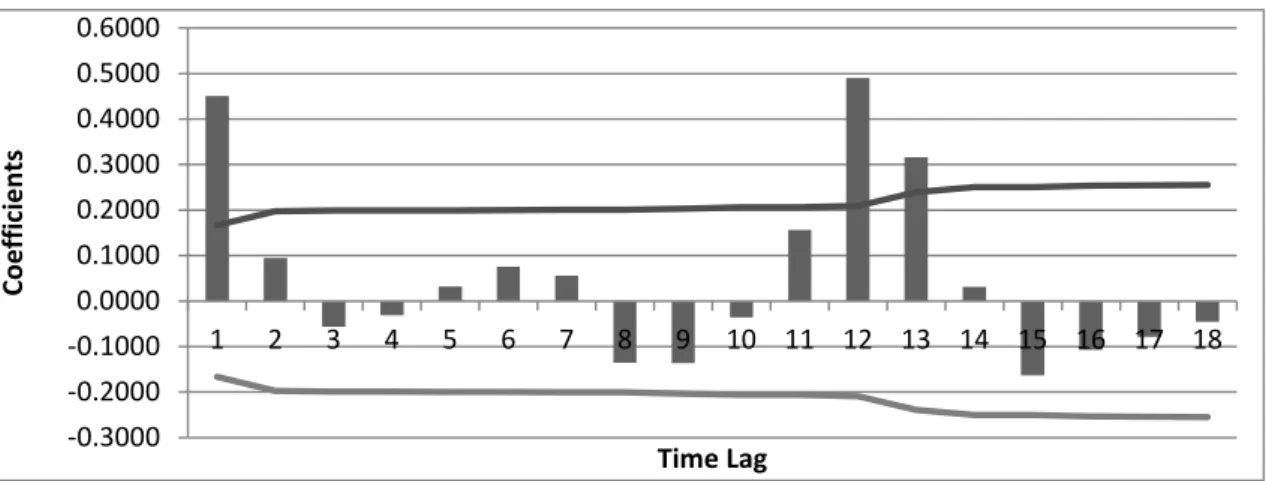
With the proposed autocorrelation analysis to detect patterns in data, the following autocorrelogram (Fig 3) was obtained, which allows to clarify the patterns of the time series.

Fig. 3. Simple autocorrelogram. Applied case 2.

The study of the autocorrelogram, according to [8], revealed that the time series does not present a trend pattern, since the coefficient of the first time lag is not close to one and the next time lags are not significantly different from zero or decrease gradually to zero, but it is observed that there is a stationary pattern, since the values diminish suddenly to zero after the first lag. Seasonality is not observed since there is not a significant trk

in any time lag period. Through the analysis of t-statistics associated to the autocorrelation coefficients (table 4) it was possible to determine that the time series have a stationary pattern. The absolute value of t- statistics for the first delay is higher than 1.96 and the rest suddenly decrease to zero, which indicates that there is correlation between the observed data.

Table 4. Autocorrelation coefficients, significance bands and t- statistics.

Given the observed data pattern in the time series (stationarity) and according to the information given by forecast methods decision tree, the following forecast methods were pre-selected: simple average (SA), naive method (NM), simple moving average (SMA), simple exponential smoothing (SES), SES with adaptative response rate (ARRSES). It should be noted that ARIMA method will not be used, since [8] suggest that the time series should have at least 50 records. Table 5 shows forecast errors given by the five used methods in this applied case.

Table 5. Forecast errors of Applied Case 2

SA NM SMA SES ARRSES MAPE (%) 16,65 18,27 12,35 16,52 3,33

rk rk2 Srk +1,96Srk -1,96Srk trk

k=1 0,37 0,14 0,17 0,33 -0,33 2,25

… … … …

k=18 -0,20 0,04 0,21 0,42 -0,42 -0,93 -0.4000

-0.2000 0.0000 0.2000 0.4000 0.6000

1 2 3 4 5 6 7 8 9 10 11 12 13 14 15 16 17 18

Coef

fi

ci

ents

(8)

Having developed the models and analyzed the results, it was established that the most suitable model to develop future sales forecast of vehicles is ARRSES method. This presents a mean absolute percentage error (MAPE) of 3,33% compared to 12,35% of SMA method. This method is also able to precisely project the stationarity. To determine the optimal parameters for the five models, “Solver” from MS Excel© software was used, which obtained the values that minimized the MSE of the model.

In order to confirm that the methods suggested by the forecast methods decision tree, for this applied case, were actually the most adequate (the most precise for the data pattern), forecasts with the rest of the methods that were not proposed by the decision tree were done: double moving average, simple linear regression, time series decomposition and Holt-Winter multiplicative method without trend.

All methods not recommended by forecast methods decision tree for the case of data pattern with stationarity have a MAPE similar to the methods recommended by the decision tree, with the exception of ARRSES that presented an estimation error closer to 0. The difference between ARRSES with the best not selected method was 74,11%. The verification of the already mentioned result validates the application of this selection mechanism.

6. Conclusions

Completing a previous analysis of data pattern of the time series, the most adequate tool is the autocorrelation analysis, that allows to determine if data have randomness, seasonality, trend or stationarity through the analysis of an autocorrelogram.

Moreover, it was proposed a decision tree that shows more clearly the forecast models more adequate for each pattern of the time series. However, it is necessary to test projections with at least two or three of the pre-selected methods to evaluate which of them is the most appropriate according to the minor forecast error.

The approach of this paper was applied to 2 Chilean companies. We found that the selected forecast methods were very accurate according to the forecast errors.

This mechanism allows taking better decisions since it came to complement the visual analysis. For further studies about this subject we are going to develop an algorithm to automatize the choice of the forecast methods.

Finally, it is important to bear in mind that even though it is true that quantitative methods are adequate tools to forecast, its final weighting should not represent more than 80%. The remaining 20% should include the adjustments and interpretations that are necessary according to the opinion and knowledge the expert has, who is responsible to measure and assess the impact it will have in planning decisions.

Acknowledgements

This research has been supported by DICYT (Scientific and Technological Research Bureau) of the University of Santiago of Chile (USACH) and Department of Industrial Engineering.

References

[1] Kahn KB, Mello J (2004). Lean Forecasting begins with lean thinking on the demand forecasting process. Journal of Business Forecasting2004; 23(4): 30-32, 40.

[2] Moon MA, Mentzer J, Smith CD, Garver MS. Seven Keys to Better Forecasting. Business Horizons1998;41(5): 44-52.

(9)

[4] Chopra S, Meindl P. (2001). Supply Chain Management. Strategy, Planning and Operation. 1st ed. Gabler; 2001.

[5] Valencia M, Ramirez S, Gonzalez D, Cardona J. Comparación de Metodologías Estadísticas en Pronóstico de la Demanda, Revista Ingeniería Industrial UPB2013; 1(1): 29

[6] Bowerman BL, O’Connell RT, Koehler AB.Pronósticos, Series de Tiempo y Regresión, un enfoque aplicado.4th ed. México, DF: Thomson; 2007.

[7] Wilson JH, Keating B.Pronósticos en los Negocios con ForecastX basado en Excel. 5th ed. Mexico: McGraw Hill; 2007. [8] Hanke JE, Reitsch AG. Pronósticos en los Negocios. 5th ed. Mexico: Prentice Hall;1996.

[9]. Pighin S., 2001. “Data Mining. Informática Aplicada a la Ingeniería de Procesos I (Orientación I)”, Universidad Tecnológica Nacional, Facultad Regional Rosario, Argentina. Available at:

http://www.frro.utn.edu.ar/repositorio/catedras/quimica/5_anio/orientadora1/monograias/pighin-datamining.pdf

[10] Aguirre J. Introducción al Tratamiento de Series Temporales: Aplicación a las Ciencias de la Salud. 1st ed. Madrid: Diaz de Santos; 1994.

[11] Garcia A., Torollo M., 2010. Estudio Sobre el Desempleo en España. Revista Internacional del Mundo Ecónomico y del Derecho 2, p.15-16.