Does corruption affect economic growth?
29
0
0
Texto completo
(2) 278. LATIN AMERICAN JOURNAL OF ECONOMICS | V. N. (N, ), –. Concern about the negative social and economic impacts of corruption has grown rapidly, and major international organizations consistently claim that corruption hinders economic growth.1 Despite these claims that corruption is detrimental to economic growth, economists have not necessarily agreed with the argument from theoretical standpoints. Theoretical studies suggest that corruption may counteract government failure and promote economic growth in the short run, given exogenously determined suboptimal bureaucratic rules and regulations. As government failure is itself a function of corruption, however, corruption should have detrimental ef fects on economic growth in the long run. In practice, economists care more about such long-term consequences of corruption than the short-term ef fects. Corruption can affect resource allocation in two ways. First, it can change (mostly) private investors’ assessments of the relative merits of various investments. This influence follows from corruption-induced changes in the relative prices of goods and services as well as of resources and factors of production, including entrepreneurial talent. Second, corruption can result in resource misallocation when decisions on how public funds will be invested, or which private investments will be permitted, are made by a corrupt government agency. The misallocation follows from the possibility that a corrupt decision-maker will consider potential “corruption payments” as one of the decision criteria. Ranking of projects based on their social value may differ from a ranking based on the corruption income that the agent expects to receive. Empirical literature in the field has consistently reported a negative correlation between economic growth and the level of corruption, and evidence on beneficial ef fects has been scarce at best (Mauro, 1995; Barreto, 1996; Tanzi, 1997). Mauro (1995) and Li et al. (2000) showed that corruption is indeed negatively associated with investment and economic growth. The authors also suggested that the direction of causality is from corruption to development, rather than vice versa.2 A large number of theoretical studies point to several channels through which corruption may adversely af fect income, but as of yet, these theoretical investigations, although suggestive, have an empirical basis. 1. The World Bank (2006) states, “The Bank has identified corruption as the single greatest obstacle to economic and social development.” Similarly, the International Monetary Fund (2006) states, “Poor governance [that of fers greater incentives and more scope for corruption] clearly is detrimental to economic activity and welfare.” 2. Mauro’s findings have been confirmed in recent work by Kaufmann et al. (1999). These findings are also consistent with those of Barreto (1996), Hall and Jones (1999) and La Porta et al. (1999)..
(3) E. Ahmad, M.A. Ullah, and M.I. Arfeen| DOES CORRUPTION AFFECT ECONOMIC GROWTH. 279. While most of the theoretical literature has taken a microeconomic approach (Shleifer and Vishny, 1991, 1993; Cadot, 1987), in Section 3 we present growth modeling of corruption to show the impact of corruption and institutional variables on economic growth. In this model, weak institutions, political instability and inef ficient bureaucracy are detrimental to economic growth. Specifically, we find corruption to be growth-enhancing at low levels of incidence and growth-reducing at high levels of incidence. This implies that the existence of a positive level of corruption that maximizes longrun growth has two separate ef fects. The main purpose of this study is to increase understanding of the relationship between corruption and economic growth using panel data. An attempt has therefore been made in the present study to understand the problem of corruption, weak institutions, inef ficient bureaucracy and political instability through empirical evidence and to of fer policy recommendations based on findings. The specific objectives of the study are: (a) specification of a model of corruption based on a theoretical foundation for cross-country analysis; (b) to determine the growth maximizing level of corruption; and (c) to determine whether it is the combined ef fect of corruption and institutional quality that causes growth. Consistent with the objectives of the study, the following hypotheses will be tested: Hypothesis 1: In the linear specification, corruption is negatively correlated with real GDP. In the case of non-linear specification, a moderate level of corruption positively af fects real GDP, while a high level of corruption is detrimental to growth. Hypothesis 2: Other things being equal, better institutional quality tends to be positively related to economic growth. The study proceeds by reviewing the existing literature on institutions, corruption, and economic growth in Section 2. Growth modeling of corruption on the basis of the theoretical framework described in Section 2 is presented in Section 3; this section also provides a detailed discussion of data, construction of variables and estimation techniques. The empirical analysis of the results is carried out in Section 4. Finally, Section 5 summarizes the main findings of the study to of fer policy recommendations..
(4) 280. 2.. LATIN AMERICAN JOURNAL OF ECONOMICS | V. N. (N, ), –. DEFINING CORRUPTION AND LITERATURE REVIEW. Corruption is a complex and multifaceted phenomenon with multiple causes and effects, as it takes on various forms and functions in different contexts. The phenomenon of corruption ranges from a single act of an illegal payment to the endemic malfunction of a political and economic system. The problem of corruption has been seen either as a structural problem of politics or economics, or as a cultural and individual moral problem. The definition of corruption consequently ranges from the broad terms of “misuse of public power” and “moral decay” to strict legal definitions of corruption as an act of bribery involving a public servant and a transfer of tangible resources (Andvig et al., 2000). The decisive role of the state is reflected in most definitions of corruption, which view it as a particular and perverted state-society relationship. Corruption is conventionally understood and referred to as the private wealth-seeking behavior of someone who represents the state and public authority. It also includes the misuse of public resources by public of ficials for private gain. The encyclopedic and working definition used by the World Bank (1997), Transparency International (1998) and others is that corruption is the abuse of public power for private benefit (or profit). Another widely used description is that corruption is a transaction between private and public sector actors through which collective goods are illegally converted into private goods (Heidenheimer et al., 1989: 6). This point is also emphasized by Rose-Ackerman (1978), who says corruption exists at the interface of the public and private sectors. Nye (1967: 416) defines corruption as “behavior that deviates from the formal duties of a public role (elective or appointive) because of private-regarding (personal, close family, private clique) wealth or status gains.” An updated version with the same elements is the definition of Khan (1996: 12): corruption is “behavior that deviates from the formal rules of conduct governing the actions of someone in a position of public authority because of private-regarding motives such as wealth, power, or status.”. 2.1. Theoretical and empirical background A natural starting point for the economic analysis of corruption is to treat it as any other crime and apply to it the standard economic model of crime developed originally in Becker (1968) and extended.
(5) E. Ahmad, M.A. Ullah, and M.I. Arfeen| DOES CORRUPTION AFFECT ECONOMIC GROWTH. 281. subsequently by many authors such as Polinsky and Shavell (1979, 1984). In this basic model, persons contemplating corruption take into account the expected benefits in the form of bribes, favors or payment in kind and compare the monetary equivalent of these gains with the expected costs in the form of the probability that they will be detected and the monetary sum (or equivalent) of the punishment should they be convicted. Such a formulation has close parallels with the application of Becker’s model to the economics of tax evasion by Allingham and Sandmo (1972). Corruption is predicted to occur if the net expected gain is positive. The theoretical and empirical literature on corruption has generated a rich debate over the last 30 years. On one hand, researchers such as Krueger (1974), Myrdal (1989), Shleifer and Vishny (1993), Tanzi (1997), and Mauro (1995, 1998) have argued that corruption is detrimental to economic growth. They point out that corruption modifies government goals and diverts resources from public purposes to private ones, thereby resulting in a deadweight loss to society.3 Furthermore, government corruption may also discourage private investment by raising the cost of public administration (since it is likely to take the form of a bribe for a public service) or by generating social discontent and political unrest, which in turn, may slow economic growth (Alesina, 1992). On the other hand, Lef f (1964), Huntington (1968), and Friedrich (1972) have suggested that it is also possible for corruption to be beneficial for economic growth. They argue that if the government has produced a package of pervasive and inef ficient regulations, then corruption may help circumvent these regulations at a low cost. Under this scenario, it is plausible that corruption may improve the ef ficiency of the system and actually help economic growth.4 Another argument in favor of corruption views bribery as “speed money,” that is, payments that speed up the bureaucratic process, or payments that are intended to “mediate” between political parties that would not reach agreement otherwise. Then, as long as the time consumed by administrative procedures is reduced by the bribe, the bribers could be made better of f. Lui (1985), for example, presented a model in which the costs of “standing in line” are minimized by 3. In a related argument, Krueger (1974) explains how unproductive, rent-seeking activities can be expected to arise in a corrupt environment. 4. In a famous passage, Huntington (1968: 69) stated it simply: “In terms of economic growth, the only thing worse than a society with a rigid, over-centralized, dishonest bureaucracy is one with a rigid, over-centralized, honest bureaucracy.”.
(6) 282. LATIN AMERICAN JOURNAL OF ECONOMICS | V. N. (N, ), –. the use of bribes. Kaufmann and Wei (1998), however, contested the empirical validity of this hypothesis. Ehrlich (1999) stated that corruption and per capita income are expected to be negatively correlated across different stages of economic development. The dif ference between corruption and crime is that corruption depends on investment in political capital as a ticket for entry to the bureaucratic ranks, unlike entry to many criminal activities, which requires little skill. The author argued that such an investment has repercussions on the incentive of productive agents to invest in human capital. The relationship between corruption and the economy is thus explained as an endogenous outcome of competition between growth-enhancing and socially unproductive investments and its reaction to exogenous factors, especially government intervention in private economic activity. Cartier-Bresson (1999) suggested five economic conditions that encourage corruption to flourish in a society. The first of these conditions is the existence of an exploitable natural resource (e.g., oil) that provides the opportunity for state authorities, both administrative and political, to obtain payments. Secondly, the general scarcity of public assets relative to demand accompanied by policies of fixed of ficial prices creates opportunities for informal rationing through bribery. Thirdly, low wages in the public sector are also likely to be associated with extensive low-level corruption payments. Fourthly, high levels of state intervention/planning (i.e., protectionism, stateowned enterprises, price controls, exchange controls, import licenses, etc.), which have characterized many developing countries, create opportunities for corruption. Finally, economies in transition are likely to experience particular problems that cause corruption as they undertake privatization and establish the relevant legal framework of corporate and contract law, etc. Empirical literature in the field has consistently reported a negative correlation between economic growth and the level of corruption, and the evidence for beneficial ef fects on growth has been scarce at best.5 Using a cross section of countries, Mauro (1995) demonstrated that after controlling for a number of economic and sociopolitical factors, the relationship between corruption and economic growth is negative. Keefer and Knack (1995) also reported a negative correlation between 5. An in-depth review of all cases can be found in Klitgaard (1988)..
(7) E. Ahmad, M.A. Ullah, and M.I. Arfeen| DOES CORRUPTION AFFECT ECONOMIC GROWTH. 283. corruption and GDP growth. Others such as Hall and Jones (1999) and Sachs and Warner (1997) have obtained similar results. Tanzi and Davoodi (1997) found evidence of bureaucratic malpractice manifesting in the diversion of public funds to the areas where bribes are easiest to collect, implying a bias in the composition of public spending towards low-productivity projects (e.g., large-scale construction) at the expense of value-enhancing investments (e.g., maintenance or improvements in the quality of social infrastructure). Thus, abuse of public of fice may not only reduce the volume of public funds available to the government (through corrupt practices in tax collection), but may also lead to misallocation of those funds. According to Lambsdorf f (1999), empirical research on the causes of corruption has focused on political institutions, government regulations, legal systems, GDP levels, salaries of public employees, gender, religion and other cultural dimensions, poverty, and the history of colonialism. Lambsdorf f stated that it is often dif ficult to assess whether corruption causes other variables or is itself the consequence of certain characteristics. Empirical research based on various corruption indexes has reported a correlation between certain forms of government regulations, poor public institutions, poverty and income inequality. But conclusions with respect to causality are vague. A major obstacle for cross-national comparative empirical research is the dif ficulty in measuring the levels of relative corruption in dif ferent countries. However, in recent years economists and political scientists have started to analyze the indexes of perceived corruption prepared by Political Risk Services6 and various business risk analysts and polling organizations. A number of econometric studies using these indexes as explanatory variables examine historical, cultural, political and economic determinants of a variety of indicators of government quality, including corruption (e.g., La Porta et al., 1999; Paldam, 1999; Treisman, 2000). Thus, most of the empirical evidence seems to be consistent with the theories that hold corruption to be purely detrimental. However, all of these empirical studies assume that corruption has only a monotonic impact upon economic growth, and therefore, they provide an incomplete 6. Political Risk Services quantifies and rates political risk using a methodology developed by Professors William D. Coplin and Michael K. O’Leary at the Maxwell School of Citizenship and Public Af fairs, Syracuse University. Political Risk Services’ methodology is the most widely accepted system of completely independent political risk forecasting..
(8) 284. LATIN AMERICAN JOURNAL OF ECONOMICS | V. N. (N, ), –. test of the hypotheses that have treated this impact as a dif ferentiated phenomenon depending on the extent of the corruption.. 3.. GROWTH MODELING OF CORRUPTION. A common view among economists is that corruption af fects output by distorting the allocation of resources. This view contrasts with the hypothesis prevalent among many economic historians and political scientists that in an economy with a rigid bureaucracy, corruption may be beneficial in that it “oils the wheels of bureaucracy.” The decomposition of output into its components, capital (physical and human) and total factor productivity (TFP) of fers a glimpse into this controversy. This study follows Hall and Jones (1999) in taking the view that TFP mainly reflects market ef ficiency. Following the empirics of Mauro (1995), we develop and modify the growth model of corruption. Since the author does not test whether there is a growth-enhancing or growth-reducing level of corruption, one wonders whether corruption still af fects economic growth adversely if more policy controls are added. It is apparent from the specification used in Mauro’s study that the linear framework can only provide a partial test of the theory, as it only captures the linear ef fect and the growth-maximizing level of corruption is forced to lie in a corner. The analysis starts from the standard production function, which extends Solow’s (1956) original approach to the growth accounting process. We can model the aggregate production function in the following way. Yit = Ait F(Kit,Lit). (1). Yit = AitKitα Lit1−α. (2). or. where Yit is the aggregate output, Ait is the total factor productivity (TFP), Kit is the capital stock, and Lit is the quantity of labor in country i at time period t. The parameter α measures the share of capital and 1 − α measures the share of labor in total output. Dividing Equation (2) by L and then taking natural logarithms, we obtain: yit = ait + αkit. (3).
(9) E. Ahmad, M.A. Ullah, and M.I. Arfeen| DOES CORRUPTION AFFECT ECONOMIC GROWTH. 285. where Y yit = ln it L it ait = ln Ait K kit = ln it L it As we have to empirically analyze the ef fects of institutional quality indicators, corruption indicators and other policy indicators of economic growth, we do so through total factor productivity growth and determine corruption and institutional quality within the model. The dynamic feature of the model arises from the inclusion of a lagged dependent variable. For convenience, in empirical analysis we specify the following relationships: ait = n0 + ∑njXitj + ∑nkXitk + nyi(t−1) + nit. (4). where: ait = total factor productivity.. Xj = set of j conditioning variables, which includes: X1 = Government expenditure (% of GDP).. X2 = Indicator of external competitiveness, measured as the trade-to-GDP ratio. X3 = Population growth rate.. X4 = Primary school enrollment rate (log form).. X5 = Secondary school enrollment rate (log form). X6 = Foreign direct investment (gross). X7 = Risk-to-investment index.. Xk = set of k variables measuring the level of corruption and institutional quality, which includes: X8 = Corruption index.. X9 = Square of corruption index.. X10 = Bureaucratic ef ficiency index.. X11 = Political stability index.. X12 = Institutional ef ficiency index..
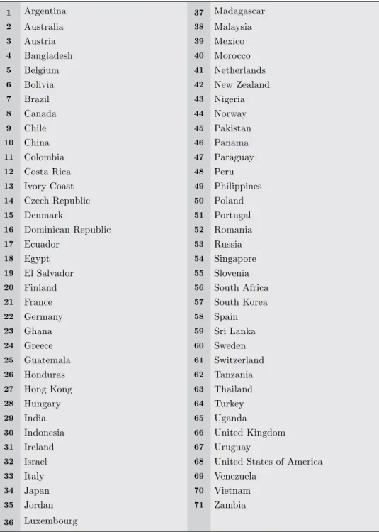
(10) 286. LATIN AMERICAN JOURNAL OF ECONOMICS | V. N. (N, ), –. βj’s are the coef ficients of the first seven conditioning variables, δK are the coef ficients of the eight variables measuring corruption and institutional quality, γ is the coef ficient of lag of GDP per worker and finally, µ is the random error term. The set of conditioning variables X4 and X5 measures the quality of human capital. By substituting Equation (4) in Equation (5), we obtain the final version of the growth model of corruption; yi,t-1 is the logarithm of GDP per worker at the start of that period. yit = n0 + ∑ n j Xitj + ∑ nk Xitk + nyi,t -1 + n. Kit + n1it Lit. (5). We attempt to capture both the growth-enhancing and growth-reducing ef fects of corruption on growth by estimating long-run growth as a linear-quadratic function of corruption, as well as the set of controls in Barro (1991, 1997 and 2004), Mankiw, Romer and Weil (1992) and Mauro (1995), where the conditioning variables include measures of human capital, indicators of external competitiveness, government spending as a share of GDP, the population growth rate, and the riskto-investment index. It is worth noting that most of the previous work on growth accounting and corruption has adopted a linear specification. We compare both specifications and show that linear-quadratic is preferred on the basis of standard statistical tests. The traditional (linear) setting does not allow for the growth-maximizing level of corruption to dif fer from zero or infinity. Population growth, education, openness, and institutional variables (government expenditure and corruption) contribute to determining steady-state, per-capita growth levels. These variables and lag of GDP per worker af fect the speed at which an economy converges toward its steady state, thereby af fecting the growth rate.. 3.1. Definition and source of data The study is based on a panel data set over the period 1984-2009 for 71 developed and developing countries. High-income countries are categorized as developed countries and the countries that fall into the low-income, lower-middle-income, and upper-middle income categories are developing countries7. An important advantage of using panel data 7. World Bank, World Development Report 2004..
(11) E. Ahmad, M.A. Ullah, and M.I. Arfeen| DOES CORRUPTION AFFECT ECONOMIC GROWTH. 287. is that they capture both time-series and cross-section variations in variables. The data are sourced from Political Risk Services’ International Country Risk Guide (ICRG)8 and the International Monetary Fund’s International Financial Statistics Yearbook (2009).. 3.2. Description of the data In order to analyze the panel data, the study employs two data sets. The smaller one, shown in Appendix A, contains 60 countries, both developed and developing. The data set in Appendix A contains 71 countries. Country choice is constrained by the limited availability of data on policy variables. In order to minimize the measurement error in each individual index, we created simple averages of closely related variables, which may yield a better estimate of the determinants of economic growth. It seems that corruption, bureaucratic quality and law and order indices represent closely related variables on the basis of the definitions of variables, and that their simple average may be reasonable proxies for what we will label bureaucratic ef ficiency. Similarly, the simple average of the democratic accountability, military in politics, external conflicts, internal conflicts and government stability indices may be a reasonable proxy for political stability. In addition to being closely related on a priori grounds, the indices that we choose to group together are more strongly correlated with each other. In some estimates we aggregate all eight indices into an average index of institutional ef ficiency, which we define as including bureaucratic ef ficiency as well as political stability. The possibility of multicollinearity makes it dif ficult to tell which of the several institutional factors examined is crucial for economic growth.9 It may be desirable to combine groups of variables into composite indices. The ICRG indices value was a maximum of 4, 6 and 12; due to averaging of the indices we convert all the indices to a maximum of 12. Descriptive statistics for all regression variables are provided in Appendix B. There is not much variation in the mean of the ICRG indices. 8. In assigning a “grade” to the country in which they are based, PRS correspondents follow general criteria outlined in the questionnaires they complete. For example, for the bureaucratic quality index, a grade of 12 is given in the case of a “smoothly functioning, efficient bureaucracy,” while a grade of 5 means “constant need for government approvals and frequent delays.” These indices were assembled by hand based on the hard copies of the questionnaires. 9. This is a common finding. Putnam (1993) reported that all his indicators of bureaucratic efficiency for the Italian regions tend to move together to a remarkable extent as well..
(12) 288. LATIN AMERICAN JOURNAL OF ECONOMICS | V. N. (N, ), –. All ICRG indices are positively correlated to each other. The simple correlation coef ficient between corruption and bureaucratic quality indices is 0.72 while the correlation coef ficient between democratic accountability and government stability indices is 0.30 (Appendix C contains the correlation matrix for the ICRG indices). A number of mechanisms may contribute to explaining the positive correlation among all categories of institutional efficiency. Corruption may be expected to be more widespread in countries where red tape slows down bureaucratic procedures. In addition, the report from the Asian Development Bank (2003) argues that corruption may even lead to more bureaucratic delay.10 In fact, when individuals offer speed money (which may prevent delay for an individual), it may increase red tape for the economy as a whole. The fact that all categories of country risk tend to move together is an interesting result. Correlation coefficients of Barro-type variables are given in Appendix D, which shows negative (-0.65) correlation between the log of capital per worker and population growth. In the given sample of 71 countries, the country reported to have the most efficient bureaucracy is Sweden, obtaining grades of 12 out of 12 for the period 1984-2009 for all bureaucratic efficiency indices we use. It also had the highest real GDP per worker during that same period. At the opposite extreme, ICRG considered Nigeria to have the least efficient institutions among the countries in the sample for that period, while Russia had the lowest growth rate of GDP per worker (-2.2). A quick glance at these appendices shows that richer countries tend to have better institutions than poorer countries, and that fast-growing countries also tend to be among those with a higher bureaucratic efficiency index. One of the most striking features of the data set is the strong association between bureaucratic efficiency and political stability.11 A potential endogeneity problem arises as economic growth may af fect the level of corruption. The direction of this ef fect is, however, unclear. Higher economic growth may increase the availability of rents, making corruption more profitable, but it also increases the amount of resources that can be devoted to control it. In either case, corruption would be correlated with the error term in the random 10. Krueger (1993) and De Soto (1989) also argue that corrupt bureaucrats will intentionally introduce new regulations and red tape in order to be able to extract more bribes by threatening to deny permits. 11. Shleifer and Vishny (1993) argue that countries with weak (and therefore unstable) governments will experience a very deleterious type of corruption, in which an entrepreneur may have to bribe several public of ficials and still face the possibility that none of them really have the power to allow the project to proceed..
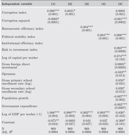
(13) E. Ahmad, M.A. Ullah, and M.I. Arfeen| DOES CORRUPTION AFFECT ECONOMIC GROWTH. 289. ef fects model (REM) and the estimates would be biased. If economic growth increases (decreases) corruption, regression coef ficients on the linear and quadratic terms for corruption would be biased upward (downward). In order to overcome this dif ficulty, several authors in the past have included an instrumental variable and conducted a two-stage least squares regression. In theory, this is a perfectly valid procedure. In practice however, it is very dif ficult to find a valid instrument. The two-dimensionality of the panel data creates two types of errors that af fect the performance of estimates. One is related to the crosssectional observation and the other to time series observations (e.g., a country-specific error can overstate the estimates in our sample). Apart from these errors, the inclusion of the lag dependent variable also worsens the problem of serial correlation; to overcome the problem of bias and endogeneity this study uses the generalized method of moments (GMM), apart from REM.. 4.. RESULTS AND DISCUSSION. The main results of applying the GMM technique are summarized in Table 1.12 It is clear from column 1 of Table 1 that the coef ficient of corruption is significantly dif ferent from zero. Note also that the coef ficient on Corruption Squared in the linear-quadratic model is different from zero at the 10% significance level. The overall explanatory power is improved if we include control variables (column 5). Mauro (1995), using specifications with linear corruption and a limited set of controls, found significant coef ficients for corruption on the order of 0.002. In his study, after controlling for other important determinants of economic growth, the coefficient on corruption became more significant. In their study of economic growth and convergence, Keefer and Knack (1997) reported that the coef ficient on corruption becomes insignificant after other variables are included in the regressions. The sign of the coef ficients, as expected, suggests the existence of a positive, growth-maximizing level of corruption. Specifically, corruption is found to become detrimental to economic growth for ICRG values lower than 10 in the baseline model (column 1).13 What happens when the square of the corruption index is dropped? In the 12. The magnitude of coef ficients for various variables dif fers substantially due to the use of dif ferent units of measurement for the variables. 13. It is important to remember that a lower ICRG value denotes a higher incidence of corruption..
(14) 290. LATIN AMERICAN JOURNAL OF ECONOMICS | V. N. (N, ), –. Table 1.. GMM estimates of the relationship between economic growth and corruption. (dependent variable is log of gdp per worker) Independent variable. (1). (2). Corruption index. 0.006*** (0.001). 0.0021* (0.001). Corruption squared. -0.0003* (0.0001). (3). (4). (5). 0.0003 (0.001) -0.001*** (0.0002) 0.004*** (0.001). Bureaucratic ef ficiency index. 0.004*** (0.001). Political stability index. 0.006*** (0.001). Institutional ef ficiency index Risk to investment index. 0.003*** (0.0009). Log of capital per worker. 0.874*** (0.182). Gross foreign direct investment. 0.0005* (0.0003). Openness. -0.033** (0.014). Gross primary school enrollment rate (log). 0.050* (0.031). Gross secondary school enrollment rate (log). 0.020* (0.012). Population growth. -0.007*** (0.002). Government expenditure. -0.002*** (0.0007). Log of GDP per worker (-1). 1.006*** (0.004). 0.999*** (0.003). 0.992*** (0.004). 0.993*** (0.003). 0.830* (0.443). Constant. -0.075** (0.034). -0.0003 (0.027). 0.043 (0.027). 0.037 (0.023). -0.300* (0.181). 969 0.9994. 969 0.9994. 969 0.9994. 969 0.9994. 969 0.9995. N Adj. R2. linear specification, corruption in the GMM specification (column 2) is quite similar and significant, and also has a negative ef fect on real GDP per worker. A one-standard-deviation increase (an improvement) in the corruption index raises the log of GDP per worker by 0.78% (obtained by multiplying 0.0021, the slope coef ficient, by 3.73, the standard deviation of the index).14 When we included the conditioning variables in our model, we obtained more significant results (column 6). The size of the coefficient Corruption 14. See column 2, Table 1..
(15) E. Ahmad, M.A. Ullah, and M.I. Arfeen| DOES CORRUPTION AFFECT ECONOMIC GROWTH. 291. Table 1. (continued) Independent variable. Corruption index Corruption squared. (6). (7). (8). 0.010*** (0.002). 0.009*** (0.002). 0.003 (0.002). 0.003* (0.0016). (10). 0.007*** (0.002). 0.012*** (0.002). 0.005*** (0.001) -0.0003*** (0.0001). Bureaucratic ef ficiency index Political stability index Institutional ef ficiency index Risk to investment index. (9). 0.001** (0.0008). Log of capital per worker. 0.002*** (0.001). 0.002*** (0.0009). 0.002** (0.0009). 0.738*** (0.193). 0.836*** (0.229). 0.790*** (0.189). Gross foreign direct investment. 0.0005* (0.0003). 0.0006* (0.0003). 0.0005 (0.0003). 0.0006** (0.0003). Openness. -0.040*** (0.014). -0.042*** (0.015). -0.044*** (0.014). -0.041*** (0.014). Primary school enrollment rate (log). -0.019 (0.025). 0.041 (0.029). 0.024 (0.026). Secondary school enrollment rate (log). 0.024** (0.007). 0.006 (0.009). 0.003 (0.008). Population growth. 0.003 (0.005). -0.007*** (0.002). -0.007*** (0.002). -0.007*** (0.002). Government expenditure. -0.004*** (0.001). -0.003*** (0.0008). -0.003*** (0.0008). -0.003*** (0.0007). Log of GDP per worker (-1). 1.025*** (0.006). -0.500 (0.465). -0.710 (0.198). 0.991*** (0.004). -0.641 (0.451). Constant. 0.012 (0.115). -0.034 (0.101). -0.252 (0.168). 0.032 (0.027). -0.154 (0.146). N Adj. R2. 969 0.9991. 969 0.9981. 969 0.9974. 969 0.9994. 969 0.9982. Source: Authors’ calculations. Note: Standard errors are in parentheses. *Significant at 10% **Significant at 5% ***Significant at 1%.. Squared (0.0003) is not changed but the significance level improves (significant at 1%). The level of corruption that maximizes economic growth is still around 8.3 for column 6. The significance levels for the corruption index proved to be sensitive to the inclusion of risk to investment and political stability indexes. A sense of the economic importance of the coef ficients can be obtained by predicting the change in long-run economic growth resulting from a decrease (worsening) in the corruption index. For countries with low levels of corruption, such as The Netherlands, Norway.
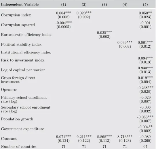
(16) 292. LATIN AMERICAN JOURNAL OF ECONOMICS | V. N. (N, ), –. Table 2.. Random ef fects estimates of the relationship between economic growth and corruption. (dependent variable is log of gdp per worker) Independent Variable. (1). (2). Corruption index. 0.064*** (0.008). 0.020*** (0.002). Corruption squared. -0.004*** (0.0005). (3). (4). (5). 0.050** (0.023) -0.001 (0.001) 0.025*** (0.003). Bureaucratic ef ficiency index. 0.039*** (0.003). Political stability index. 0.061*** (0.012). Institutional ef ficiency index Risk to investment index. 0.094*** (0.013). Log of capital per worker. 0.930*** (0.013). Gross foreign direct investment. 0.019*** (0.004). Openness. -0.238*** (0.028). Primary school enrollment rate (log). -0.029 (0.087). Secondary school enrollment rate (log). -0.006 (0.032). Population growth. -0.053*** (0.007). Government expenditure. -0.004** (0.002). Constant Number of countries. 9.071*** (0.124). 9.211*** (0.122). 8.868*** (0.113). 8.713*** (0.123). -0.089 (0.360). 71. 71. 71. 71. 67. and Sweden (corruption index near 12), such a worsening up to the growth-maximizing level of corruption implies an increase in long-run growth of 0.40 percentage points per year. For countries with average levels of corruption, such as Nigeria (corruption index of 3.1) and Pakistan (4.4), an improvement (increase) in the corruption index would raise long-run economic growth by 1.66 and 0.85 percentage points per year respectively. In the random ef fects estimation, we obtain significant coef ficients of 0.064 for Corruption and -0.004 for Corruption Squared, which imply a growth-maximizing level of corruption of 7.5, very similar to that of Table 1; however, the results of the Corruption Squared term in columns 5 and 6 of Table 2 are highly insignificant..
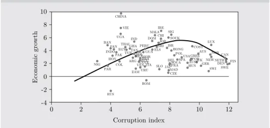
(17) 293. E. Ahmad, M.A. Ullah, and M.I. Arfeen| DOES CORRUPTION AFFECT ECONOMIC GROWTH. Table 2. (continued) Independent Variable. Corruption index Corruption squared. (6). (7). (8). 0.002*** (0.0008). 0.006*** (0.0004). 0.001* (0.001). 0.008*** (0.0006). Institutional ef ficiency index 0.367*** (0.039). Primary school enrollment rate (log) Secondary school enrollment rate (log) Population growth Government expenditure Constant Number of countries. 0.002*** (0.0005). 0.001*** (0.0006). 0.005*** (0.0006). 0.004*** (0.0007). 0.412*** (0.003). 0.401*** (0.001). 0.400*** (0.001). -0.014 (0.013). 0.0001 (0.0002). -0.0004 (0.0004_. -6.6E-05 (0.0002). -0.339*** (0.077). -0.0002 (0.003). 0.001 (0.001). -0.002* (0.001). -0.476* (0.261). 0.015*** (0.004). -0.011*** (0.004). 1.370*** (0.089). 0.0002 (0.001). 0.008*** (0.001). Log of capital per worker. Openness. 0.041*** (0.003). -0.001 (0.004). Political stability index. Gross foreign direct investment. (10). 0.204*** (0.069). Bureaucratic ef ficiency index. Risk to investment index. (9). -0.011 (0.037). 0.001 (0.001). -0.001* (0.0007). -0.001* (0.0006). 0.022*** (0.006). -0.001*** (0.0002). -0.001*** (0.0001). -7.9E-05 (0.0001). 1.680 (1.086). 0.007 (0.012). -0.014 (0.019). 8.723*** (0.113). 0.043** (0.020). 67. 68. 67. 71. 67. Source: Authors’ calculations. Note: Standard errors are in parentheses. *Significant at 10% **Significant at 5% ***Significant at 1%.. As shown in the appendix, countries such as Costa Rica, Hong Kong, Poland, Spain and Greece (which have rates of economic growth well above the average) have corruption indexes that are remarkably close to the estimated optimal level of corruption. Figure 1 plots the average real GDP per worker against the average corruption index and its square term for the 60 countries. The figure provides the growthmaximizing level of corruption, which is 8.3 according to our GMM estimates (Table 1, column 6)..
(18) 294. LATIN AMERICAN JOURNAL OF ECONOMICS | V. N. (N, ), –. Figure 1. Relationship between corruption and economic growth 10. CHINA. Economic growth. 8 6 4 2. NIG. 0. ROM. -2 -4. IRE SIG MALA CHI SOUK DOM IND JOR LUX BAN THAI SRI ISR GHA PERU PAN COST HONG EGY TAN ELS AUS INDO GUA NOR TUR BOL POL CAN PAK MEXMOR USA GREE BRA POR HON UK NEW NETH BEL SPA ECU ARG COTE FIN AUST GER SOUA DEN COL VEN ITA SLO HUN JAPFRA SWI SWE PAR MAD URU ZAM CZE VIE. UGA. RUS. 0. 2. 4. 6. 8. 10. 12. Corruption index Source: Authors’ calculations.. 4.1. Institutional ef ficiency and economic growth Table 1 also shows the simple relationship between economic growth and institutional variables in further detail. Column 3 of Table 2 shows that a one-standard-deviation increase (an improvement) in the bureaucratic ef ficiency index is associated with an increase in the log of GDP per worker of 1.2% (obtained by multiplying 0.004, the slope coef ficient, by 3.04, the standard deviation of the index). The estimated magnitude of the ef fects of bureaucratic ef ficiency on economic growth is even higher (and remains significant) when we add conditioning variables. The coef ficient is still significant at the conventional levels, as shown in column 5. Therefore, these results do not provide any support for the claim that in the presence of a slow bureaucracy, corruption would become beneficial, as suggested by Lef f (1964) and Huntington (1968). Corruption and bureaucratic inefficiency both adversely and significantly affect real GDP per worker. Having provided some evidence in favor of the claim that corruption hinders economic growth, we now turn to analyzing the channels through which this takes place. In the context of an endogenous growth model, bureaucratic inefficiency could affect economic growth indirectly (by lowering the investment rate) or directly (for example, by leading to misallocation of investment among sectors) (Easterly, 1993; Mauro, 1995). In the case of the political stability index, a one-standard-deviation decrease (worsening) in the index is associated with a decrease in.
(19) E. Ahmad, M.A. Ullah, and M.I. Arfeen| DOES CORRUPTION AFFECT ECONOMIC GROWTH. 295. the log of GDP per worker of 0.86%15 and if we include conditioning variables then the ef fect is even greater, i.e., 1.29%.16 The random ef fects estimation (Table 2) also gives the highly significant results with even greater impact on economic growth. Controlling for all the variables in all techniques, the political stability index and the bureaucratic ef ficiency index are always positively and significantly associated with GDP per worker, although the level of significance of the political stability index improves when human capital indicators are included in the list of independent variables (Table 2, columns 7 and 8). The magnitude of the coef ficient on bureaucratic ef ficiency is in this case twice as large as in column 3 of Table 1. Table 1 (columns 9 and 10) shows the simple relationship between economic growth and the institutional efficiency index. A one-standarddeviation increase (improvement) in the institutional ef ficiency index is associated with an increase in the log of GDP per worker by 1.74% and 2.98% respectively (obtained by multiplying 0.007 and 0.012, the slope coef ficients, by 2.49, the standard deviation of the index). The corruption, bureaucratic efficiency, political stability and institutional ef ficiency indices are significantly associated with GDP per worker. Again, we analyze the robustness of these simple relationships to alternative control variables, using the two dif ferent methodologies. The null hypothesis of no relationship between GDP per worker and corruption can be rejected at a level of significance lower than the one at which the null hypothesis of no relationship between investment and corruption can be rejected. This finding is consistent with the results reported by Levine and Renelt (1992), Mauro (1995) and Barro (1997). The finding that corruption is negatively and significantly associated with economic growth is consistent with the view that corruption lowers the marginal product of capital (for example, by acting as a tax on investment proceeds).. 4.2. Conditioning variables and economic growth In the growth model of corruption we consider, the control variables are a measure of international openness, the ratio of government spending to GDP, a subjective indicator of risk to investment, gross 15. Obtained by multiplying 0.004, the slope coefficient, by 2.15, the standard deviation of the index, shown in Table 1, column 4. 16. This value is calculated by multiplying 0.006, the slope coefficient, by 2.15, the standard deviation of the index, given in Table 1, column 5..
(20) 296. LATIN AMERICAN JOURNAL OF ECONOMICS | V. N. (N, ), –. foreign direct investment and indicators of human capital, population growth and lag of GDP per worker (log). The results show that the coef ficient of log of capital per worker in the growth equation is positive and statistically significant, indicating that capital growth is the key variable af fecting economic growth. As in much of the cross-country literature, the regression results show that greater human capital—as measured by gross secondary school enrollment—is associated with faster economic growth. Moreover, since our GMM panel estimator controls for endogeneity, this finding suggests that the exogenous component of schooling exerts a positive impact on economic growth. The results in tables 1 and 2 indicate a significantly negative association between government spending and GDP per worker. The argument is that although government consumption has no direct ef fect on private productivity (or private property rights), it lowers saving and growth through distortionary ef fects from taxation or government expenditure programs (Barro 1991). Big government spawns corruption via bureaucrats manipulating spending in order to collect more bribes (Li et al., 2000). Thus, the results suggest that macroeconomic policy is also important as large government tends to hurt economic growth. According to the GMM results, the direct ef fects of a one-standard-deviation increase in risk to investment (improvement) on the log of GDP per worker is an increase of 0.62 percentage point (Table 1, column 5).. 5.. CONCLUDING REMARKS. We derive a growth model of corruption on the basis of the theoretical underpinnings. The main result obtained here is that the growthmaximizing level of corruption is not necessarily equal to zero, confirming the predictions of political economy theory developed over the last three decades. The evidence from this study demonstrates the statistical importance of corruption in the development of a robust model that explains real GDP per worker. The empirical literature that reported a linear relationship between corruption and economic development failed to differentiate between growth-enhancing and growth-reducing levels of corruption. In this study we present evidence that suggests the existence of a humpshaped relationship between corruption and long-run economic growth. This finding remains unchanged under several specifications..
(21) E. Ahmad, M.A. Ullah, and M.I. Arfeen| DOES CORRUPTION AFFECT ECONOMIC GROWTH. 297. Drawing longitudinal implications from cross-sectional data is hazardous, but for what it is worth, the estimates of this study suggest that if for example, Bangladesh were to improve the integrity and efficiency of its bureaucracy to the level of that of China (corresponding to a onestandard-deviation increase in the bureaucratic efficiency index), its real GDP per worker would rise by almost one and a half percentage points. The catch, of course, is that high levels of corruption and bureaucratic inef ficiency are themselves likely to impede investment and growth (Mauro, 1995). But corruption does not necessarily prevent economic growth when other factors are conducive. Indeed, the three “most corrupt” countries in the International Country Risk Guide data for the mid-1980s—Indonesia, Paraguay and Ghana—had average economic growth of 1% during the 1980s (although substantially below the worldwide average of 3.2%). The analysis for the panel data on countries lends significant support to the proposition that the quality of public institutions plays a crucial role in the growth performance of any country. This is evident not only in the high statistical significance of the estimated parameters for the institutional variables but also in their robustness to changes in model specifications. There are several channels, not all of which are analyzed in this study, through which corruption hinders economic development. They include reduced domestic investment, reduced foreign direct investment, overblown government expenditure, distorted allocation of government expenditure away from education, health, and the maintenance of infrastructure and towards less-ef ficient public projects that provide more scope for manipulation and bribe-taking opportunities. Hong Kong, Portugal, and Singapore have demonstrated that corruption can be reduced significantly. Encouraging research and the dissemination of its findings can provide valuable direction to policymakers..
(22) 298. LATIN AMERICAN JOURNAL OF ECONOMICS | V. N. (N, ), –. REFERENCES Alesina, A.N. Roubini, S. Ozler, and P. Swagel (1992), “Political Instability and Economic Growth,” NBER Working Paper No. 4173. Allingham, M. and A. Sandmo (1972), “Income Tax Evasion: A Theoretical Analysis,” Journal of Public Economics, Vol. 1: 323-38. Andvig, J.O. Fjeldstad, I. Amundsen, T. Sissener and T. SØreide(2000), “Research on Corruption: A Policy Oriented Survey,” Norwegian Agency for Development Co-operation (NORAD) Report. Asian Development Bank (2003), Ef fective Prosecution of Corruption, India. Barreto, R.A. (1996), “Endogenous Corruption, Inequality and Growth,” European Economic Review, Vol. 44, No. 1: 35-60. Barro, R.J. (1991), “Economic Growth in a Cross Section of Countries,” Quarterly Journal of Economics, Vol. 106, No. 2: 407-43. . (1997), Determinants of Economic Growth: A Cross-Country Empirical Study, 2nd Edition. Cambridge: MIT Press. . (1998), Notes on Growth Accounting, Harvard University Discussion Paper. Barro, R.J. and X. Sala-i-Martin (2004), Economic Growth, 2nd Edition. Cambridge: MIT Press. Becker, G.S. (1968), “Crime and Punishment: An Economic Approach,” Journal of Political Economy, Vol. 76: 169-217. Cadot, O. (1987), “Corruption as a Gamble,” Journal of Public Economics, Vol. 33, No. 2: 223 - 244. Cartier-Bresson, J. (1995), “L’Economie de la Corruption,” in D. Della Porta and Y. Mény, eds., Démocratie et Corruption en Europe. Paris: La Découverte. De Soto, H. (1989), The Other Path. New York: Harper and Row. Easterly, W. and S. Rebelo (1993), “Fiscal Policy and Economic Growth: An Empirical Investigation,” Journal of Monetary Economics, Vol. 32: 417-458. Ehrlich, I. and F.T. Lui (1999), “Bureaucratic Corruption and Endogenous Economic Growth,” Journal of Political Economy, Vol. 107, No. 6: 270-293. Friedrich, C.J. (1972), The Pathology of Politics, Violence, Betrayal, Corruption, Secrecy and Propaganda. New York: Harper and Row. Hall, R.E. and J. Charles (1999), “Why do Some Countries Produce so Much More Output Per Worker than Others?” Quarterly Journal of Economics, Vol. 114, No. 1: 83-116. Heidenheimer Arnold J. (1989), “What is the Problem About Corruption?” In Political Corruption: A Handbook, M. Johnson and V.T. LeVine, eds. New Brunswick, New Jersey: Transaction. Huntington, Samuel P. (1968), Political Order in Changing Societies. New Haven: Yale University Press. International Monetary Fund (2009), International Financial Statistics 2009, Washington, D.C..
(23) E. Ahmad, M.A. Ullah, and M.I. Arfeen| DOES CORRUPTION AFFECT ECONOMIC GROWTH. 299. Kaufmann, D. and S-J. Wei (1998), “Does ‘Grease Money’ Speed Up the Wheels of Commerce?” NBER Working Paper No. 7093. Kaufmann, D., A. Kraay, and P. Zoido-Lobaton. (1999), “Governance Matters.” World Bank Policy Research Paper No. 2196. Washington, D.C.: World Bank. Khan, M.H. (1996), “A Typology of Corrupt Transactions in Developing Countries”, IDS Bulletin: Liberalization and the New Corruption, Vol. 27, No.2. Klitgaard, R. (1988), Controlling Corruption. Berkeley: University of California Press. Knack, S. and P. Keefer (1995), “Institutions and Economic Performance: CrossCountry Tests Using Alternative Institutional Measures,” Economics and Politics Vol. , No. 3: 207-27. Krueger, A.O. (1993), Political Economy of Policy Reform in Developing Countries, Cambridge: MIT Press. . (1974), “The Political Economy of the Rent-Seeking Society,” American Economic Review, Vol. 64: 291-303. La Porta, F., R. Lopez-de-Silanes, A. Shleifer, and R. Vishny (1999), “The Quality of Government,” Journal of Law, Economics and Organization, Vol. 15: 222-279. Lambsdorf f, J.G. (1999a), “Corruption in Empirical Research – A Review,” Transparency International Working Paper, Berlin. Lef f, N. (1964), “Economic Development through Bureaucratic Corruption,” American Behavioral Scientist, Vol. 8, No. 3:8-14. Levine, R. and D. Renelt (1992), “A Sensitivity Analysis of Cross-Country Growth Regression,” American Economic Review, Vol. 82, No. 4: 942-963. Li, H., L. Colin, and H-F. Zou (2000), “Corruption, Income Distribution and Growth,” Economics and Politics, Vol. 12, No.2: 155-181. Lui, F.T. (1985), “An equilibrium queuing model of bribery,” Journal of Political Economy, Vol. 93, No. 4: 760-81. Mankiw, N., D. Romer, and D.N. Weil (1992), “A Contribution to the Empirics of Economic Growth,” Quarterly Journal of Economics, Vol. 107: 407-437. Mauro, P. (1995), “Corruption and Growth,” Quarterly Journal of Economics, Vol. 110, No. 3: 681-712. Mauro, P. (1998), “Corruption: Causes, Consequences, and Agenda for Further Research,” International Monetary Fund Finance and Development (March): 11-14. Murphy, K., A. Shleifer, and W. Vishny (1991), “The Allocation of Talent, Implications for Growth,” Quarterly Journal of Economics, Vol. 106: 503-530. Myrdal, G. (1989), “Corruption: Its Causes and Ef fects,” in Political Corruption: A Handbook, A. Heidenheimer, M. Johnston, V.T. LeVine, eds. Rutgers, New Jersey: Transaction Publishers. Nye, J.S. (1967), “Corruption and Political Development,” American Political Science Review, Vol. 61, No. 2: 417-427..
(24) 300. LATIN AMERICAN JOURNAL OF ECONOMICS | V. N. (N, ), –. Paldam, M. (1999a), “The Big Pattern of Corruption: Economics, Culture and the Seesaw Dynamics,” University of Aarhus School of Economics and Management Economics Working Paper No. 1999-11. Polinsky, A.M. and S. Shavell (1979), “The Optimal Trade-of f Between the Probability and Magnitude of Fines,” American Economic Review, Vol. 69: 880-891. . (1984), “The Optimal Use of Fines and Imprisonment,” Journal of Public Economics, Vol. 69: 880-891. Political Risk Services (2009), International Country Risk Guide Dataset, www. icrgonline.com. Putnam, Robert D. (1993), Making Democracy Work: Civic Tradition in Modern Italy. Princeton, New Jersey: Princeton University Press. Rose-Ackerman, S. (1978), Corruption: A Study in Political Economy. New York: Academic Press. . (1996), “Democracy and ‘Grand’ Corruption,” International Social Science Journal, Vol. 48, No. 3. Sachs, J. and M.W. Andrew (1997), “Fundamental Sources of Long-Run Growth,” American Economic Review, Vol. 87: 184-188. Shleifer, A. and R.W. Vishny (1993), “Corruption,” The Quarterly Journal of Economics, Vol. 108: 599–617. Solow, Robert M. (1956), “A Contribution to the Theory of Economic Growth,” Quarterly Journal of Economics, Vol. 70: 65-94.Tanzi, V. and H. Davoodi (1997), “Corruption, Public Investment, and Growth,” IMF Working Paper 97/139, Washington, D.C. Treisman, D. (2000), “The Causes of Corruption: A Cross-National Study,” Journal of Public Economics, Vol. 76: 399-457. Wei, S. (1997), How Taxing is Corruption on International Investors, National Bureau of Economic Research Working Paper No. 6030. World Bank (1997), “Helping Countries Combat Corruption”, The World Bank, Poverty Reduction and Economic Management Program, Washington, D.C. . (1997), The State in a Changing World: World Development Report 1997. Oxford: Oxford University Press. . (2009), World Development Indicators 2009, Washington, D.C. . (2009), World Development Report 2009, Washington, D.C..
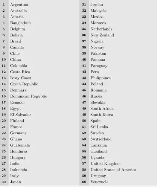
(25) E. Ahmad, M.A. Ullah, and M.I. Arfeen| DOES CORRUPTION AFFECT ECONOMIC GROWTH. APPENDIX A Data Table A1. Data set for generalized method of moments 1. Argentina. 31. Jordan. 2. Australia. 32. Malaysia. 3. Austria. 33. Mexico. 4. Bangladesh. 34. Morocco. 5. Belgium. 35. Netherlands. 6. Bolivia. 36. New Zealand. 7. Brazil. 37. Nigeria. 8. Canada. 38. Norway. 9. Chile. 39. Pakistan. 10. China. 40. Panama. 11. Colombia. 41. Paraguay. 12. Costa Rica. 42. Peru. 13. Ivory Coast. 43. Philippines. 14. Czech Republic. 44. Poland. 15. Denmark. 45. Romania. 16. Dominican Republic. 46. Russia. 17. Ecuador. 47. Slovakia. 18. Egypt. 48. South Africa. 19. El Salvador. 49. South Korea. 20. Finland. 50. Spain. 21. France. 51. Sri Lanka. 22. Germany. 52. Sweden. 23. Ghana. 53. Switzerland. 24. Guatemala. 54. Tanzania. 25. Honduras. 55. Thailand. 26. Hungary. 56. Uganda. 27. India. 57. United Kingdom. 28. Indonesia. 58. United States of America. 29. Italy. 59. Uruguay. 30. Japan. 60. Venezuela. Sources: Political Risk Services, the World Bank and the International Monetary Fund.. 301.
(26) 302. LATIN AMERICAN JOURNAL OF ECONOMICS | V. N. (N, ), –. Table A2. Data set for random ef fects model 1. Argentina. 37. Madagascar. 2. Australia. 38. Malaysia. 3. Austria. 39. Mexico. 4. Bangladesh. 40. Morocco. 5. Belgium. 41. Netherlands. 6. Bolivia. 42. New Zealand. 7. Brazil. 43. Nigeria. 8. Canada. 44. Norway. 9. Chile. 45. Pakistan. 10. China. 46. Panama. 11. Colombia. 47. Paraguay. 12. Costa Rica. 48. Peru. 13. Ivory Coast. 49. Philippines. 14. Czech Republic. 50. Poland. 15. Denmark. 51. Portugal. 16. Dominican Republic. 52. Romania. 17. Ecuador. 53. Russia. 18. Egypt. 54. Singapore. 19. El Salvador. 55. Slovenia. 20. Finland. 56. South Africa. 21. France. 57. South Korea. 22. Germany. 58. Spain. 23. Ghana. 59. Sri Lanka. 24. Greece. 60. Sweden. 25. Guatemala. 61. Switzerland. 26. Honduras. 62. Tanzania. 27. Hong Kong. 63. Thailand. 28. Hungary. 64. Turkey. 29. India. 65. Uganda. 30. Indonesia. 66. United Kingdom. 31. Ireland. 67. Uruguay. 32. Israel. 68. United States of America. 33. Italy. 69. Venezuela. 34. Japan. 70. Vietnam. 35. Jordan. 71. Zambia. 36. Luxembourg.
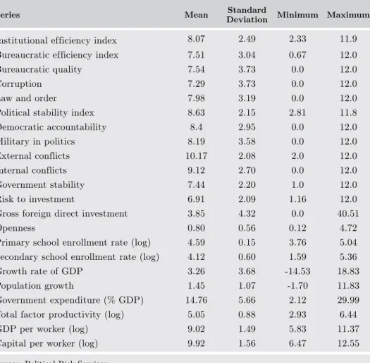
(27) E. Ahmad, M.A. Ullah, and M.I. Arfeen| DOES CORRUPTION AFFECT ECONOMIC GROWTH. 303. APPENDIX B Table B1. Descriptive statistics of regression variables Mean. Standard Deviation. Minimum. Maximum. Institutional ef ficiency index. 8.07. 2.49. 2.33. 11.9. Bureaucratic ef ficiency index. 7.51. 3.04. 0.67. 12.0. Bureaucratic quality. 7.54. 3.73. 0.0. 12.0. Corruption. 7.29. 3.73. 0.0. 12.0. Law and order. 7.98. 3.19. 0.0. 12.0. Political stability index. 8.63. 2.15. 2.81. 11.8. Democratic accountability. 8.4. 2.95. 0.0. 12.0. Military in politics. 8.19. 3.58. 0.0. 12.0. External conflicts. 10.17. 2.08. 2.0. 12.0. Internal conflicts. 9.12. 2.70. 0.0. 12.0. Government stability. 7.44. 2.20. 1.0. 12.0. Risk to investment. 6.91. 2.09. 1.16. 12.0. Gross foreign direct investment. 3.85. 4.32. 0.0. 40.51. Openness. 0.80. 0.56. 0.12. 4.72. Primary school enrollment rate (log). 4.59. 0.15. 3.76. 5.04. Secondary school enrollment rate (log). 4.12. 0.60. 1.59. 5.36. Series. Growth rate of GDP. 3.26. 3.68. -14.53. 18.83. Population growth. 1.45. 1.07. -1.70. 11.83. Government expenditure (% GDP). 14.76. 5.66. 2.12. 29.99. Total factor productivity (log). 5.05. 0.88. 2.93. 6.44. GDP per worker (log). 9.02. 1.49. 5.83. 11.37. Capital per worker (log). 9.92. 1.56. 6.47. 12.55. Source: Political Risk Services. There are 1,089 observations in the sample. A high value for the Political Risk Service (PRS) index means the country has solid institutions. The Barro (1991) repressors are risk to investment, primary and secondary education, population growth, government expenditures, openness and gross foreign direct investment (GFDI)..
(28) 0.45. Risk to investment. 0.74. 0.73 0.73. 0.61. Internal conflicts. Law and order. 0.35. Government stability. Military in politics. 0.60. 0.40. External conflicts. 0.32. 0.74. 0.23. 0.43. 0.72. 0.71. 1. Democratic accountability. 1 0.76. Corruption. Bureaucratic quality. Bureaucratic Corruption quality. 0.43. 0.78. 0.67. 0.59. 0.30. 0.51. 1. Democratic accountability. 0.33. 0.50. 0.55. 0.62. 0.28. 1. External conflicts. 0.68. 0.32. 0.41. 0.41. 1. Government stability. Table C1. Correlation matrix for political risk service indices. APPENDIX C. 0.40. 0.68. 0.82. 1. Internal conflicts. 0.42. 0.74. 1. Law and order. 0.44. 1. Military in politics. 1. Risk to investment. 304 LATIN AMERICAN JOURNAL OF ECONOMICS | V. N. (N, ), –.
(29) 0.59 -0.65 0.33 0.80 0.33 0.21. Population growth. Primary school enrollment rate (log). Secondary school enrollment rate (log). Foreign direct investment (gross). Openness. 1.00. Government expenditure. Capital per worker (log). Capital per worker (log). 0.25. 0.31. 0.50. 0.08. -0.36. 1.00. Government expenditure. -0.09. -0.27. -0.69. -0.34. 1.00. Population growth. Table D1. Correlation matrix for Barro type variables. APPENDIX D. 0.00. 0.19. 0.55. 1.00. 0.22. 0.36. 1.00 0.30. 1.00. Primary school Secondary school Foreign direct enrollment rate enrollment rate investment (log) (log) (gross). 1.00. Openness. E. Ahmad, M.A. Ullah, and M.I. Arfeen| DOES CORRUPTION AFFECT ECONOMIC GROWTH. 305.
(30)
Figure
+3
Documento similar