Structure of the obscured galactic disk with pulsating variables

Texto completo

(1)STRUCTURE OF THE OBSCURED GALACTIC DISK WITH PULSATING VARIABLES Gergely Hajdu.

(2) FACULTAD DE FÍSICA INSTITUTO DE ASTROFÍSICA. STRUCTURE OF THE OBSCURED GALACTIC DISK WITH PULSATING VARIABLES BY. GERGELY HAJDU Thesis submitted to the Faculty of Physics at Pontificia Universidad Católica de Chile in partial fulfillment of the requirements for the degree of Doctor in Astrophysics Thesis submitted to the Combined Faculties for the Natural and for Mathematics of the Ruperto-Carola University of Heidelberg for the degree of Doctor of Natural Sciences. Thesis Advisor. MÁRCIO CATELAN Santiago de Chile, September 2019 c MMXIX, GERGELY HAJDU.

(3) Se autoriza la reproducción total o parcial, con fines académicos, por cualquier medio o procedimiento, incluyendo la cita bibliográfica del documento..

(4) FACULTAD DE FÍSICA INSTITUTO DE ASTROFÍSICA. STRUCTURE OF THE OBSCURED GALACTIC DISK WITH PULSATING VARIABLES BY. GERGELY HAJDU. Members of the Committee. Márcio Catelan. (IA – PUC). Eva K. Grebel. (ARI – UH). Mario Trieloff. (GEOW – UH). Thomas H. Puzia. (IA – PUC). Manuela Zoccali. (IA – PUC). Santiago de Chile, September 2019. c MMXIX, GERGELY HAJDU.

(5)

(6) ACKNOWLEDGEMENTS I would like to thank all the support I have received during the wonderful years I have spent at the Pontificia Universidad Católica de Chile, Santiago, as well as during my one year exchange at the Astronomisches Rechen-Institut der Universität Heidelberg. First and foremost, I would like to thank my supervisor, Prof. Márcio Catelan, for all the support, encouragement, and motivation I have received from him. Secondly, I am also deeply thankful for my co-advisor and exchange host, Prof. Eva Grebel, for allowing me to spend a very productive, wonderful year in Heidelberg. The work presented in this thesis would not have been possible without that of Dr. István Dékány. We started working together on VVV data at Católica, and continued to do so after he moved to Heidelberg, which has resulted in all the results presented here. I cannot overstate his inspirational effect on my work, as well on my development as an astronomer. I would like to thank my mother for all the patience she has displayed while I was conducting my studies in Chile and Germany. I cannot end the acknowledgements without mentioning my comrades among the students, both at the IA, as well as at the ARI. At the former, I could always count upon Diego Calderón, Rodrigo Carvajal, Camila Navarrete, Katerine Joachimi, and many others, to have stimulating conversations about our research, as well as just to remind ourselves to relax, and spend time together, in order to ease our minds of the everyday stress experienced by the majority of students, in this otherwise unforgiving academic environment. During my time at ARI, I have received much support from Michael Hanke, Zdenek Prudil and Josefina Michea in the daily goings of both the university, as well as Heidelberg. I would like to thank my officemates at ARI, Bekdaulet Shukirgaliyev and Clio Bertelli Motta for a wonderful time. Finally, I would like to acknowledge the “First La Serena School for Data Science"", where I have been introduced for the first time to many of the statistical and data science methods iv.

(7) ACKNOWLEDGEMENTS. v. utilized throughout this thesis. In this endevour, the book “Statistics, Data Mining, and Machine Learning in Astronomy” (Ivezić et al. 2014) has also been indispensable. During my studies, I have been financially supported by CONICYT-PCHA (Doctorado Nacional 2014-63140099), by the Graduate Student Exchange Fellowship Program between the Institute of Astrophysics of the Pontificia Universidad Católica de Chile and the Zentrum für Astronomie der Universität Heidelberg, funded by the Heidelberg Center in Santiago de Chile and the Deutscher Akademischer Austauschdienst, as well as by the Ministry for Economy, Development, and Tourism’s Programa Iniciativa Milenio through grant IC1200009. Additional support is acknowledged by Proyecto Basal PFB-06/2007 and AFB-170002, by FONDECYT grants #1141141 and #1171273, by CONICYT Anillo grant ACT 1101, by CONICYT’s PCI program through grant DPI20140066, and the CONICYT’s “Beca Asistencia a eventos y cursos cortos para estudiantes de doctorado - convocatoria 2015”. Processing and analysis of data were partly performed on the Milky Way supercomputer, which is partly funded by the Sonderforschungsbereich SFB 881 “The Milky Way System” (subproject Z2) of the Deutsche Forschungsgemeinschaft..

(8) CONTENTS ACKNOWLEDGEMENTS. iv. LIST OF TABLES. ix. LIST OF FIGURES. x. 1 INTRODUCTION. 1. 1.1 The Milky Way disk . . . . . . . . . . . . . . . . . . . . . . . . . . . . . . . . .. 1. 1.2 RR Lyrae variables . . . . . . . . . . . . . . . . . . . . . . . . . . . . . . . . . .. 5. 1.3 Cepheid variables . . . . . . . . . . . . . . . . . . . . . . . . . . . . . . . . . .. 9. 1.4 The VISTA Variables in the Vía Láctea survey . . . . . . . . . . . . . . . . . .. 13. 1.5 The layout of the thesis . . . . . . . . . . . . . . . . . . . . . . . . . . . . . . .. 14. 2 RR LYRAE LIGHT CURVES IN THE NEAR-INFRARED. 17. 2.1 Light-curve properties of RR Lyrae variables . . . . . . . . . . . . . . . . . . .. 17. 2.2 Model representation of near-IR RRab light-curves . . . . . . . . . . . . . . . .. 21. 2.2.1 The light-curve training set . . . . . . . . . . . . . . . . . . . . . . . . .. 22. 2.2.2 Data preparation . . . . . . . . . . . . . . . . . . . . . . . . . . . . . . .. 23. 2.2.3 Application of PCA to the KS -band light curves . . . . . . . . . . . . . .. 27. 2.2.4 Approximation of the J-band light curve shape . . . . . . . . . . . . . .. 32. 2.3 Robust fitting of RRL KS -band light curves . . . . . . . . . . . . . . . . . . . .. 35. 2.4 Metallicity estimation from KS -band photometry . . . . . . . . . . . . . . . . .. 39. 2.4.1 VVV photometry of bulge RR Lyrae variables . . . . . . . . . . . . . . .. 40. 2.4.2 Revision of I-band RR Lyrae photometric metallicity estimates . . . . . .. 41. 2.4.3 Iron abundance estimation from the KS -band light-curve shapes . . . . .. 48. vi.

(9) 2.4.4 Validation of the metallicity estimates . . . . . . . . . . . . . . . . . . . . 3 RR LYRAE VARIABLES IN THE VVV DISK FIELDS. 52 57. 3.1 Searching for RR Lyrae stars in the VVV disk fields . . . . . . . . . . . . . . . .. 57. 3.1.1 The VVV disk data set . . . . . . . . . . . . . . . . . . . . . . . . . . . .. 57. 3.1.2 Variability and period search . . . . . . . . . . . . . . . . . . . . . . . .. 58. 3.1.3 Classification of RRL candidates . . . . . . . . . . . . . . . . . . . . . . .. 59. 3.1.4 Calculation of individual RRL properties . . . . . . . . . . . . . . . . . .. 61. 3.2 Properties of the RRL sample . . . . . . . . . . . . . . . . . . . . . . . . . . . .. 63. 3.2.1 Spatial distribution . . . . . . . . . . . . . . . . . . . . . . . . . . . . . .. 63. 3.2.2 Metallicity distribution . . . . . . . . . . . . . . . . . . . . . . . . . . . .. 69. 3.2.3 Spatial variations in metallicity . . . . . . . . . . . . . . . . . . . . . . .. 72. 3.2.4 Comparison of the MDF to independent results . . . . . . . . . . . . . .. 75. 3.3 Discussion and future directions . . . . . . . . . . . . . . . . . . . . . . . . . .. 78. 4 RECALIBRATION OF VISTA PHOTOMETRY. 81. 4.1 VVV photometric inconsistencies . . . . . . . . . . . . . . . . . . . . . . . . . .. 81. 4.2 VISTA calibration procedures . . . . . . . . . . . . . . . . . . . . . . . . . . . .. 82. 4.2.1 The 2MASS Point Source catalog in the VISTA system . . . . . . . . . .. 83. 4.3 Revision of H-band VISTA observations . . . . . . . . . . . . . . . . . . . . . .. 84. 4.4 VISTA zero point bias in dense stellar fields . . . . . . . . . . . . . . . . . . . .. 86. 4.5 Recalibration of VVV JHKS observations . . . . . . . . . . . . . . . . . . . . .. 91. 4.5.1 Effects of the photometric corrections . . . . . . . . . . . . . . . . . . . .. 93. 4.5.2 Recommendations for future usage of VISTA observations . . . . . . . .. 96. 5 CEPHEIDS IN THE VVV SURVEY. 100. 5.1 Cepheid search in the corrected VVV photometry . . . . . . . . . . . . . . . . 100 5.1.1 Classification of Cepheid candidates . . . . . . . . . . . . . . . . . . . . . 101 5.1.2 Cepheid period-luminosity relationships . . . . . . . . . . . . . . . . . . 105. vii.

(10) 5.1.3 The near-infrared extinction law . . . . . . . . . . . . . . . . . . . . . . 107 5.2 Distribution of the VVV classical Cepheid sample . . . . . . . . . . . . . . . . . 112 5.2.1 Apparent Cepheid pairs . . . . . . . . . . . . . . . . . . . . . . . . . . . 118 5.3 The radial age trend of VVV Classical Cepheids . . . . . . . . . . . . . . . . . . 120 5.4 The VVV Classical Cepheids and the spiral arms . . . . . . . . . . . . . . . . . 124 5.5 Summary and future outlook . . . . . . . . . . . . . . . . . . . . . . . . . . . . 128 6 CONCLUSIONS. 130. 6.1 Outlook . . . . . . . . . . . . . . . . . . . . . . . . . . . . . . . . . . . . . . . . 132 AUTHOR’S PUBLICATIONS. 134. REFERENCES. 138. viii.

(11) LIST OF TABLES 2.1 Collection of RR Lyrae near-IR photometric observations . . . . . . . . . . . .. 18. 2.2 Parameters of the hyperparameter grid search . . . . . . . . . . . . . . . . . .. 50. 2.3 Number of RR Lyrae variables in different metallicity bins . . . . . . . . . . . .. 51. 3.1 Parameters of the GMM components towards the bulge and the disk . . . . . .. 71. 5.1 Candidate Classical Cepheid pairs in the VVV Cepheid sample . . . . . . . . . 119. ix.

(12) LIST OF FIGURES 1.1 Face-on map of the atomic hydrogen distribution in the Milky Way disk . . . .. 2. 1.2 Galactic map of high mass star forming regions with measured parallaxes . . .. 3. 1.3 SDSS images of galaxies with warping disks . . . . . . . . . . . . . . . . . . .. 4. 1.4 Schematic Hertzsprung-Russel diagram of the positions of pulsating variable classes . . . . . . . . . . . . . . . . . . . . . . . . . . . . . . . . . . . . . . . .. 6. 1.5 U BV IKS light curves of a typical RR Lyrae . . . . . . . . . . . . . . . . . . . .. 8. 1.6 U BVRI JK light curves of a typical Classical Cepheid variable . . . . . . . . .. 10. 1.7 Galactic distribution of Classical Cepheids in the local neighborhood . . . . . .. 12. 2.1 Example of local LASSO fits of RR Lyrae J and KS light curves . . . . . . . . .. 24. 2.2 Comparison of light-curve fits with circular normal and Fourier bases. . . . . .. 26. 2.3 KS -band normalized, and J-band zero-point aligned RR Lyrae light curves . . .. 27. 2.4 RR Lyrae KS band principal components . . . . . . . . . . . . . . . . . . . . .. 29. 2.5 Principal component amplitude distribution . . . . . . . . . . . . . . . . . . . .. 31. 2.6 Residuals of the J-band light-curve approximations . . . . . . . . . . . . . . .. 34. 2.7 Continuous Fourier representation of the principal components and the J-band regression coefficients . . . . . . . . . . . . . . . . . . . . . . . . . . . . . . . .. 35. 2.8 Example light-curve fits of RR Lyrae stars . . . . . . . . . . . . . . . . . . . . .. 38. 2.9 I-band photometric metallicity distribution of bulge RR Lyrae 1 . . . . . . . . .. 43. 2.10 Separation of Oosterhoff classes . . . . . . . . . . . . . . . . . . . . . . . . . .. 44. 2.11 I-band photometric metallicity distribution of bulge RR Lyrae 2 . . . . . . . . .. 45. 2.12 Photometric metallicities of bulge RR Lyrae with the Kepler calibration . . . .. 47. 2.13 The KS -band light-curve parameter – metallicity training sample . . . . . . . .. 49. 2.14 Revision of the KS -band metallicity estimates . . . . . . . . . . . . . . . . . . .. 53. x.

(13) 2.15 RR Lyrae KS band principal components . . . . . . . . . . . . . . . . . . . . .. 55. 3.1 Examples of VVV disk RR Lyrae light curves . . . . . . . . . . . . . . . . . . .. 60. 3.2 Principal component amplitude – period distribution of disk RR Lyrae . . . . .. 62. 3.3 Distribution of VVV disk RR Lyrae on the Galactic plane . . . . . . . . . . . .. 64. 3.4 Distribution of VVV disk RR Lyrae in Galactic coordinates . . . . . . . . . . . .. 66. 3.5 Color excess and magnitude distribution of disk RR Lyrae . . . . . . . . . . . .. 67. 3.6 Galactic height and distance distribution of VVV disk RR Lyrae . . . . . . . . .. 68. 3.7 Kernel density estimates of the MDF of the bulge and disk RR Lyrae samples .. 69. 3.8 Separation of metallicity components by GMM modeling . . . . . . . . . . . .. 72. 3.9 The GMM weights and means for the Galactic bulge RR Lyrae . . . . . . . . .. 73. 3.10 The GMM weights and means for the Galactic disk RR Lyrae . . . . . . . . . .. 74. 3.11 Kernel density estimates of the disk GMM components as a function of Galactocentric distance and the distance from the Galactic plane . . . . . . . . . . . .. 76. 4.1 Example of H-band RR Lyrae light-curve inconsistencies . . . . . . . . . . . .. 82. 4.2 H-band photometric difference map of a VISTA pawprint . . . . . . . . . . . .. 85. 4.3 Chip 5 and 6 H-band images . . . . . . . . . . . . . . . . . . . . . . . . . . . .. 86. 4.4 H-band magnitude difference between VISTA and 2MASS . . . . . . . . . . .. 87. 4.5 The H and J-band photometric bias of tile b307 . . . . . . . . . . . . . . . . .. 88. 4.6 Examples of blending in 2MASS . . . . . . . . . . . . . . . . . . . . . . . . . .. 89. 4.7 Evolution of the calculated zero points of VISTA . . . . . . . . . . . . . . . . .. 90. 4.8 Dependency of magnitude offsets on the cross-match distance . . . . . . . . .. 92. 4.9 Examples of zero-point corrected Cepheid light curves . . . . . . . . . . . . . .. 94. 4.10 RR Lyrae average magnitude differences in the bulge . . . . . . . . . . . . . . .. 97. 4.11 RR Lyrae average color differences in the bulge . . . . . . . . . . . . . . . . . .. 99. 5.1 Distribution of Cepheids in Galactic coordinates . . . . . . . . . . . . . . . . . 104 5.2 Color excess and magnitude distribution of VVV Cepheid variables . . . . . . . 108. xi.

(14) 5.3 The determination of the extinction law with Cepheids . . . . . . . . . . . . . 110 5.4 Distribution of VVV Type II Cepheid sample . . . . . . . . . . . . . . . . . . . 111 5.5 Distribution of VVV Classical Cepheid sample . . . . . . . . . . . . . . . . . . 113 5.6 Galactic height and distance distribution of VVV Classical Cepheids . . . . . . 116 5.7 The Galactic warp traced by VVV Classical Cepheids . . . . . . . . . . . . . . 117 5.8 The age distribution of VVV Classical Cepheids across the disk . . . . . . . . . 122 5.9 The radial age trend of Classical Cepheids in the VVV sample . . . . . . . . . . 123 5.10 Classical Cepheids birth regions with a spiral pattern period of 230 Myr . . . . 125 5.11 Classical Cepheids birth regions with a spiral pattern period of 270 Myr . . . . 126 5.12 Classical Cepheids birth regions with a spiral pattern period of 320 Myr . . . . 127. xii.

(15) ABSTRACT Bright pulsating variables, such as Cepheids and RR Lyrae, are prime probes of the structure of both the young and old stellar components of the Milky Way. However, the far side of the Galactic disk has not yet been mapped using such variables as tracers, due to the severe extinction caused by foreground interstellar dust. In this thesis, the near-infrared light curves from the VISTA Variables in the Vía Láctea survey are utilized to penetrate these regions of high extinction and thus discover thousands of previously “hidden” Cepheid and RR Lyrae variables. The analysis of the light curves of RR Lyrae variables, was performed with a newly developed fitting algorithm, and their metallicities determined from their near-infrared light-curve shapes, using a newly developed method. These photometric metal abundances, combined with their positions within the Galactic disk, lend support to theories of an early, inside-out formation of the Galactic disk. The newly discovered Cepheids were classified into the old (Type II) and young (Classical) subtypes. A new near-infrared extinction law was determined using the Type II Cepheids, taking advantage of their concentration around the Galactic center. The distribution of the Classical Cepheids in the Galactic disk follows both the Galactic warp and the flare of the Galactic disk at large Galactocentric radii. A first attempt has been made to connect the current locations of the Classical Cepheids to the spiral arm structure of the Milky Way.. xiii.

(16) RESUMEN Las estrellas variables pulsantes brillantes, tales como Cefeidas y RR-Lyras, son sondas fundamentales de la estructura de las componentes vieja y joven de la Vía Láctea. Sin embargo, el lado más alejado del disco de la Galaxia aún no ha sido mapeado usando tales variables debido a la severa extinción causada por polvo interestelar en frente de ellas. En esta tesis, las curvas de luz en infrarrojo cercano de la muestra VISTA Variables in the Vía Láctea son utilizadas para penetrar esas regiones y descubrir miles de Cefeidas o RR Lyras previamente “escondidas”. El análisis de las curvas de luz de las variables RR Lyras fue ejecutado con un algoritmo de ajuste, y sus metalicidades determinadas de siluetas de sus curvas de luz en el infrarrojo cercano usando métodos recientemente desarrollados. Estas abundancias fotométricas de metales, con sus posiciones en el disco Galáctico, apoyan las teorílas de la formación de adentro hacia fuera del disco de la Galaxia. Las Cefeidas descubiertas fueron clasificadas en los subtipos viejo (Tipo II) y nuevo (Clásicas). Una nueva ley de extinción en el infrarrojo cercano fue determinada usando Cefeidas Tipo II, utilizando su concentración en el centro Galáctico. La distribución de las Cefeidas Clásicas en el disco Galáctico sigue el pandeo Galáctico y el ensanchamiento del disco de la Galaxia en grandes radios Galactocéntricos. Un primer intento se efectuó con el fin de conectar las ubicaciones actuales de las Cefeidas Clásicas con la estructura de brazos espirales de la Vía Láctea.. xiv.

(17) ZUSAMMENFASSUNG Helle pulsierende variable Sterne, sogenannte Variablen wie z.B. Cepheiden und RR-Lyrae Sterne, stellen ein Hauptwerkzeug für die Untersuchung der Struktur, sowohl der jungen als auch der alten Sternkomponenten, der Milchstraße dar. Die uns gegenüberliegende Seite der galaktischen Scheibe wurde noch nicht mithilfe von Variablen kartiert, aufgrund von starker Vordergrundextinktion hervorgerufen durch interstellaren Staub. In dieser Dissertation werden die Nahinfrarot-Lichtkurven der Beobachtungskampagne VISTA Variables in the Vía Láctea verwendet, um diese Regionen mit hoher Extinktion zu durchdringen und so Tausende von zuvor "verborgenen" Cepheid- und RR Lyrae-Variablen in diesen Bereichen zu untersuchen. Die Analyse der Lichtkurven von RR-Lyrae-Variablen wurde mit einem neu entwickelten Anpassungsalgorithmus durchgeführt, und ihre Metallizitäten wurden anhand ihrer Lichtkurvenformen im Nahinfrarot unter Verwendung einer neu entwickelten Methode bestimmt. Diese photometrischen Metallhäufigkeiten schätzen, zusammen mit den Positionen der Variablen innerhalb der Galaktischen Scheibe, die Theorie über eine frühe, von innen nach außen gerichtete Bildung der Galaktischen Scheibe. Die neu entdeckten Cepheiden wurden in alte (Typ II) und junge (klassischer Typ) Untertypen eingeteilt. Ein neues Nahinfrarot-Extinktionsgesetz wurde unter Verwendung der TypII-Cepheiden unter Ausnutzung ihrer Eigenschaften der Konzentration um das galaktische Zentrum bestimmt. Die Verteilung der klassischen Cepheiden in der galaktischen Scheibe folgt sowohl ihrer Verzerrung als auch ihrer unregelmäßigen Verdickung bei großen galaktozentrischen Radien. Schlussendlich wurde ein erster Versuch unternommen, die derzeitigen Positionen der klassischen Cepheiden mit der Spiralarmstruktur der Milchstraße zu verbinden.. xv.

(18) 1 Introduction 1.1 The Milky Way disk The possibility that our home, the Milky Way galaxy, might show a spiral structure was probably first proposed by Alexander (1852), but it has taken a century until this idea was finally proven by observations of the distribution of stars of spectral types O and B in the Solar neighborhood (Morgan et al. 1952), as well as by mapping the distribution of neutral hydrogen (Kerr 1962). These methods, using young stellar tracers, as well as radio observations combined with kinematic distance estimates, remain the two main ways for studying the spiral arm structure of the Milky Way. Both methods face serious limitations: for example, radial velocity mapping is blind towards the central region of the Galaxy, as gas (and stars) move mostly perprendicularly to the line of sight, resulting in zero radial velocities. Furthermore, in these studies, the distance is calculated by assuming circular motion of the gas in the Galactic disk, combining radial velocities measured from radio emission lines (such as neutral hydrogen 21 cm emission) with a Galactic rotation curve. Deviations from circular rotation however, are expected, as spiral arms are known to excite non-circular streaming motions both in the case of Milky Way (Fresneau et al. 2005) as well as in that of other galaxies (Kim and Kim 2014; Erroz-Ferrer et al. 2015). Figure 1.1 shows a modern map of the Milky Way disk, as traced by neutral hydrogen emission, highlighting the limitations of this approach. In contrast, young stellar tracers, such as young open clusters, OB stars, and Classical Cepheids (introduced in Section 1.3), have consistent, individually determined distances, and they have been used before to delineate the spiral arm structure in the Solar neighborhood 1.

(19) INTRODUCTION. 2. Figure 1.1: Face-on map of atomic hydrogen distribution in the Milky Way disk. The color scale is proportional to the calculated surface density of the hydrogen (figure from Koo et al. 2017).. (see, e.g., Majaess et al. 2009). However, very high extinction values in the Galactic plane have so far prevented the detection of these objects at large distances in the Galactic disk. The perfect stellar tracers of the spiral structure in these regions are the high mass star forming regions (HMSFR), as their water and methanol maser emissions (Elitzur 1992) allow radiointerferometric observations to directly measure their parallaxes up to ∼ 20 kpc away, i.e., to the distance of the farthest star forming regions on the other side of the Milky Way (Sanna et al. 2017). Figure 1.2 shows the distribution of the maser sources with measured parallaxes in the Galactic disk. As can be seen, these observations are not constrained by kinematical uncertainties, in contrast to the kinematically-constrained radial velocity mapping of the gas in the Galactic disk (compare to Figure 1.1). However, this figure also highlights some.

(20) INTRODUCTION. 3. Figure 1.2: Galactic map of high mass star forming regions with measured maser parallaxes (figure from Sanna et al. 2017).. of the problems related to these tracers: they are relatively rare, when compared to other stellar tracers of the spiral structure. Furthermore, the low number of such objects with measured parallaxes is, at least, partially caused by the high number of interferometric radio observations needed to obtain the parallax of a single HMSFR. Besides the spiral structure, the disk of the Milky Way exhibits two additional major large-scale features: the Galactic warp and the flaring in its outer parts. Both effects modify the flat shape of the disk, which is otherwise followed by the inner regions. In the outer regions, the scale height of the Galactic disk increases, leading to a thicker outer disk (see,.

(21) INTRODUCTION. 4. Figure 1.3: SDSS thumbnail images of galaxies with warping disks (figure from Reshetnikov et al. 2016).. e.g., López-Corredoira and Molgó 2014, as well as references there). Furthermore, in the outer regions of the Milky Way, the disk is warped upwards in the north and downward in the south, as shown by both the distribution of atomic gas (Kerr 1957; Oort et al. 1958), as well as that of the stars (Reylé et al. 2009; Li et al. 2019). Figure 1.3 shows a selection of disk galaxies exhibiting the warping feature present in the disk of the Milky Way. It was proposed by Gilmore and Reid (1983) that the older stars belonging to the Galactic disk are kinematically separated from the younger thin-disk stars, calling this component the thick disk. The thick disk is characterized by older ages, lower metal abundances, as well as larger scale height. The formation of these two components in a cosmological framework was investigated by Brook et al. (2012), by performing hydrodynamical simulations of a Milky Way-like forming disk galaxy, resulting in an inside-out formation scenario, where the thick.

(22) INTRODUCTION. 5. disk formed earlier, followed by the thin disk, with both components being observable in present times. Spectroscopic observations (Bovy et al. 2012) lend support to this scenario. The recent identification of stars originating from a massive dwarf galaxy that has been accreted onto the Milky Way about 8 − 11 Gyr ago (Belokurov et al. 2018; Helmi et al. 2018), called the “Gaia Sausage” or Enceladus, suggests that a large fraction of the stars found in the thick disk might have originated from such mergers, similarly to the simulations of Villalobos and Helmi (2008). Due to their diagnostic value, RR Lyrae variables (Section 1.2) hold crucial information about the old stellar populations in which they reside. Therefore, finding and characterizing the RR Lyrae variables throughout the Galactic disk can provide the missing pieces to our understanding of its formation and evolution, particularly in establishing the relationship between the thick disk, halo, and bulge components, all of which are known to host old stellar populations. Similarly to RR Lyrae stars, Classical Cepheids (Section 1.3) can also contribute vastly to our understanding of the Galactic disk. In contrast to the RR Lyrae variables, however, these young stars can reveal the spiral structure of the Galactic disk (Majaess et al. 2009).. 1.2 RR Lyrae variables RR Lyrae variables are classical radial pulsators with pulsation periods between 0.2 and 1.0 day, found in the intersection of the horizontal branch and the Cepheid instability strip (IS, see Figure 1.4), with absolute magnitudes of MV ∼ 0.6. They are one of the most useful types of variable stars, as their intrinsic brightness and characteristic light-curve shapes allow their discovery out to large distances (Smith 2004; Catelan and Smith 2015). They are often found in old stellar populations, as the canonical formation scenario of RR Lyrae stars requires ages greater than 10 Gyr. As such, they serve as one of the most useful tracers of old stellar populations. They can be often found in large quantities in globular clusters (Clement et al. 2001)..

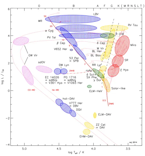
(23) INTRODUCTION. 6. Figure 1.4: Schematic Hertzsprung-Russel diagram showing the positions of major classes of pulsating variables. The zero-age main sequence is shown by the red continuous line, with the numbers next to it showing the corresponding masses in solar units. The zero-age horizontal branch is shown by the dash-dotted line, while the dashed lines denote the edges of the Cepheid instability strip. Horizontal shading (≡) represents acoustically driven modes, perpendicular shading (\\\) opacity-driven p modes, inverse perpendicular shading (///) buoyancy-driven g modes, and vertical shading (|||) strange modes (see, e.g., Catelan and Smith 2015, for the description of these mechanisms). Individual post-MS stellar evolutionary tracks are shown by the dotted lines. (Figure from Jeffery and Saio 2016.). The first discovered member of this variable star type was U Lep (Kapteyn 1890), followed.

(24) INTRODUCTION. 7. by the discovery of a seventh-magnitude star in the constellation Lyra by W.F. Flemming (Pickering et al. 1901), which later received the name RR Lyrae and became the prototype of this class of variable stars. Within a few short years of these initial discoveries, until 1913 more than 500 variables of the class had been found in globular clusters (Bailey and Pickering 1913) by the photographic monitoring program led by S.I. Bailey. RR Lyrae variables are traditionally categorized into three subtypes: the RRab variables pulsate in the radial fundamental mode, the RRc stars pulsate in the first radial overtone, while the members of the RRd subtype pulsate simultaneously in both modes. The original RRa, RRb, RRc subtypes (Bailey 1902) were revised by Schwarzschild (1940), who suggested that the larger-amplitude RRa and the lower-amplitude RRb classes are both pulsating in the fundamental mode, while the RRc variables are pulsating in the radial first overtone mode. Their pulsations are caused by the κ (Baker and Kippenhahn 1962) and γ (Cox et al. 1966) mechanisms, mainly driven by the H and He partial ionization zones in the stellar interior (for a succinct description, see Section 5.9.2 of Catelan and Smith 2015). During their pulsation cycles, RR Lyrae stars experience changes in both surface temperature and radius. The combination of these two effects leads to the observed light-curve shapes, which will also depend on the observed wavelength. Figure 1.5 shows the change in the light-curve shape of a typical RRab variable. In the U band, the change in the surface temperature dominates, while towards progressively longer wavelengths, the contribution of the change in the radius of the variable becomes commensurable, as more and more the Rayleigh-Jeans tail of the Planck function becomes dominant (see also Das et al. 2018). This also results in lowered amplitudes towards the infrared bands, posing a challenge to their detection in infrared surveys, as they become more easily confused with other types of variables, such as eclipsing binaries, especially at the lower photometric precisions achievable for ground-based near-infrared observations. Besides their characteristic shapes, and hence easy identification, what makes RR Lyrae variables excellent distance indicators is the existence of the period-luminosity-metallicity (PLZ) relations: the intrinsic magnitudes and colors of the stars can be approximated as a.

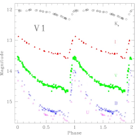
(25) INTRODUCTION. 8. Figure 1.5: Typical folded U BV IKS light curves of an RRab variable (figure from Catelan et al. 2013).. function of their pulsation periods and their metallicities (Catelan et al. 2004; Marconi et al. 2015). In case no spectroscopically measured metallicity estimates are available, in the optical bands it can be estimated as a function of the period and the light-curve shape of the variables (Jurcsik and Kovács 1996; Smolec 2005; Morgan et al. 2007). Even before 1990, thousands of RR Lyrae variables were known to exist within the Galactic disk, bulge, halo and the globular clusters of the Milky Way. With the advent of large-scale optical detectors, microlensing projects like EROS-2 (Kim et al. 2014), MACHO (Alcock et al. 2003) and OGLE (Udalski et al. 2015), as well as other transient and asteroid-hunting projects like LINEAR (Sesar et al. 2013), the Catalina Sky Survey (Drake et al. 2013; Torrealba et al. 2015), and Pan-STARRS1 (Sesar et al. 2017), thousands more were discovered. The current number of known Galactic RR Lyrae variables is over 100 000, with the two largest con-.

(26) INTRODUCTION. 9. tributors being the OGLE project (Soszyński et al. 2014) and the Gaia astrometric satellite (Clementini et al. 2019). Nothwithstanding, the fact that these surveys have greatly increased our undestanding of the old stellar population of the Galactic bulge and halo, the large amount of extinction found in the Galactic plane have so far prevented the systematic investigation of the RR Lyrae population of the Galactic disk (see e.g., Figure 26 of Clementini et al. 2019). As an example, at the distance of the Galactic bulge, the extinction in the plane of the Galaxy plane can reach A(KS ) ∼ 3.5 mag (Gonzalez et al. 2012), corresponding to A(V) > 30 mag, making this region inaccessible to any optical survey.. 1.3 Cepheid variables Cepheid variables are similar to RR Lyrae stars in the sense that they are also located within the IS, however, their periods are found between 1.0 and 100 days (Catelan and Smith 2015). Their pulsations are supported by the κ and γ mechanisms, just as in the case of RR Lyrae variables. They are categorized into two main groups: Classical (also known as Type I or δ) Cepheids and Type II Cepheids. Classical Cepheids are young (< 200 Myr), evolved population I stars of masses 2 − 20M (Turner 1996), crossing the instability strip multiple times during their post-main sequence evolution (see Figure 1.4 for their position on the Hertzsprung-Russel diagram). The brightest Classical Cepheids reach absolute magnitudes of about MV ∼ − 6 mag, while the faintest ones at MV ∼ − 2 mag are still considerably brighter than the brightest RR Lyrae variables. In contrast to the Classical Cepheids, Type II Cepheids are old, evolved low-mass stars. At the beginning of the 20th century, the distinction between the two classes of Cepheids was unknown. In the spectroscopic study of Joy (1937), hydrogen emission lines were noticed in the spectra of the variable W Virginis. Later, Joy (1940) reported similar features during the pulsation cycle of a Cepheid variable in the globular cluster Messier 3 to those of W Vir..

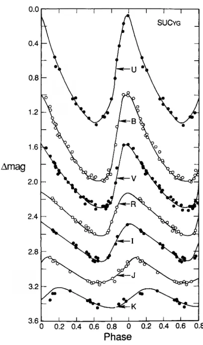
(27) INTRODUCTION. 10. Figure 1.6: Folded U BVRI JK light curves of a typical Classical Cepheid (figure from Madore and Freedman 1991).. Finally, after the indentification of Population I and II stars by Baade (1944), it has been firmly established that the Cepheid variable and W Vir belong to a separate subgroup of Cepheid variables, with the latter becoming the prototype of its class..

(28) INTRODUCTION. 11. Similarly to the RR Lyrae stars, the light curves of Classical Cepheids exhibit characteristic shapes in different bands, as shown in Figure 1.6. However, around P ∼ 8 days, a small bump appears on the the light curves of Classical Cepheids near the end of the descending branch. With increasing periods, this bump moves closer to the maxima of the light curves, eventually becoming the main maxima for Cepheids with P & 11 days. This phenomenon is called the Hertzsprung progression (Hertzsprung 1926; also see Figure 7 of Soszyński et al. 2010), and is thought to be caused by a resonance between the fundamental and second radial overtone modes (Bono et al. 2000; Gastine and Dintrans 2008). The period-luminosity (PL) relation of Classical Cepheids was discovered by Henrietta Leavitt (Leavitt and Pickering 1912). The existence of this relation allowed Hubble (1926) to determine that the Andromeda “cloud” was indeed a galaxy, separated from, and located outside of, the Milky Way. In the years since, Classical Cepheids have kept their status as one of the most powerful tools to measure extragalactic distances, and hence in the calibration of the extragalactic distance scale, which resulted in continued interest in the ever more accurate calibration of the PL relation (Macri et al. 2015; Riess et al. 2018; Groenewegen 2018). Another relation followed by Classical Cepheids is the period-age relation (Bono et al. 2005; Anderson et al. 2016): longer period Classical Cepheids are on average younger. As younger post-main sequence stars are also more massive, they also cross the IS at higher luminosities, becoming brighter, and therefore longer-period Classical Cepheids. However, there are substantial uncertainties in this relation related to our incomplete knowledge of the initial rotation rates of stars on the upper main sequence (Anderson et al. 2016). Furthermore, ideally, the crossing number of the Classical Cepheids (second or third crossing) should be known beforehand to chose the correct relation for the determination of the age; however, this is only known for stars with a long history of repeated observations, and hence observed period changes (Fadeyev 2013). Recently, Udalski et al. (2018) announced the discovery of more than 1000 new Classical Cepheids, more than doubling the number of previous known objects of this type in the.

(29) INTRODUCTION. 12. Figure 1.7: The Galactic distribution of Classical Cepheids (solid circles) and young open clusters (circled dots) in the Solar neighborhood, showing the local spiral structure. Left: Only long period (young) Classical Cepheids are shown (P ≥ 13 d). Right: As on the right panel, but short period (older) Classical Cepheids are also included (P ≥ 5 d). (Figure from Majaess et al. 2009.). Milky Way. Using this data, Skowron et al. (2018) derived key properties of the Galactic disk, while also showing that the Classical Cepheids in the southern Galactic disk do indeed follow the Galactic warp (Kerr 1957; Oort et al. 1958; Reylé et al. 2009). Furthermore, they have identified three dominant star formation episodes which have taken place in the Galactic disk in the last 100 million years. As young stars, the distribution of Classical Cepheid variables partially still follow the distribution of their original birth places, which for most of them, were the star-forming regions found within the spiral arms. Skowron et al. (2018) showed how Cepheids formed in the three major star-formation episodes have reached their current positions, migrating out of their respective spiral arms. However, similarly to the case of RR Lyrae variables, only a handful of studies have explored the Classical Cepheids in the most obscured regions of the Milky Way photometrically (see, e.g, Dékány et al. 2015a,b; Matsunaga et al. 2016), and even fewer spectroscopically (Inno et al. 2019), making our view.

(30) INTRODUCTION. 13. of the structure of the disk of the Milky Way incomplete, as there are at least 15 000 Classical Cepheids expected to reside within the Milky Way (Majaess et al. 2009).. 1.4 The VISTA Variables in the Vía Láctea survey The VISTA Variables in the Vía Láctea ESO Public Survey (VVV; Minniti et al. 2010) started in 2010 and concluded in 2016, and utilized the 4m-class Visible and Infrared Survey Telescope for Astronomy (VISTA; McPherson et al. 2006) of the European Southern Observatory (ESO). The observations taken by VISTA using the near-infrared imager VIRCAM are reduced by the VISTA Data Flow System (Emerson et al. 2004) at the Cambridge Astronomical Survey Unit (CASU). As one of the largest ESO Public Surveys, the YZJHKS single-epoch observations, as well as the KS -band time series photometry, provided by VVV have given us a unique insight into the inner Milky Way, which is otherwise obscured by the extinction caused by the dust. Therefore VVV complements the optical variability surveys, such as that carried out by the OGLE project (Udalski et al. 2015) RR Lyrae variables towards the VVV bulge fields have already been utilized in a variety of ways to study the 3D distribution of the old bulge stellar population (Dékány et al. 2013), their properties in the outer bulge regions (Gran et al. 2016), the distance to the Galactic center (Majaess et al. 2018), as well as the old stellar population residing therein (Contreras Ramos et al. 2018b). In contrast, there have been fewer studies concerning RRL stars in the disk regions of the VVV survey. Minniti et al. (2017a) conducted a preliminary study of about 25% of the VVV disk area, in the region defined by the rectangular area −2◦.24 . b . −1◦.05, 295◦ . l . 350◦ in Galactic coordinates, identifying 404 RRL stars. Furthermore, RR Lyrae variables have been utilized to confirm a globular cluster candidate (Minniti et al. 2017b) in the Galactic disk. The recent development of a machine learned RR Lyrae classifier (Elorrieta et al. 2016) allows the distinction of RRab stars from other types of variables in the KS -band time series observations obtained by the VVV survey..

(31) INTRODUCTION. 14. Similarly to the RR Lyrae variables, investigations of Classical and Type II Cepheids in the VVV survey have been most constrained to the Galactic bulge area. As up to this point, no machine learned classifier has been published that can identify Cepheid variables, and classifying them into Classical and Type II subclasses, utilizing only KS -band observations, other criteria must be utilized to distinguish the two subclasses of variables. Dékány et al. (2015a) identified two long-period variable stars, which have almost exactly the same periods, color excesses, and apparent brightnesses, while being separated only by an angular distance of 1800. 3 on the sky. Due to these peculiar properties, it has been concluded that these two variables are Classical Cepheids, still found in the open cluster where they have formed, but the other, dimmer stars are invisible in the VVV observations due to the high amounts of extinction. Similarly, Dékány et al. (2015b) identified a sample of Classical Cepheids located towards the Galactic bulge, which showed higher extinction values than expected from reddening maps (Gonzalez et al. 2012). Meanwhile, Bhardwaj et al. (2017a) used Type II Cepheids identified by the OGLE survey (Soszyński et al. 2017) to constrain their period-luminosity relationships, while Braga et al. (2019) identified Type II Cepheids in the direction of the Galactic center.. 1.5 The layout of the thesis This thesis presents a summary of the efforts undertaken during my PhD studies towards the discovery and characterization of RR Lyrae and Cepheid variables in the near-infrared observations of the VVV survey. This work has been conducted in close collaboration with researchers both at the Instituto de Astrofísica de la Pontificia Universidad Católica de Chile, as well as the Astronomisches Rechen-Institut der Universät Heidelberg. The individual chapters each closely track a specific publication (either already published or in preparation), presenting the results of a particular aspect of the work. These chapters, highlighting my contributions, are:.

(32) INTRODUCTION. 15. • Chapter 2 presents my results on the characterization of the near-infrared light-curve shapes of RRab stars. I developed a novel, robust fitting method of KS -band RRab lightcurves, based on their light-curve representations as a sum of principal components. This fit also estimates the J-band light-curve shape, allowing the determination of accurate mean J magnitudes even if only one observation is available in that band. I have found that the amplitudes of the principal component fits, together with the pulsation period, allow the estimation of the metallicities of RRab stars based only on KS -band light curves. The results presented in this chapter were published in Hajdu et al. (2018). • Chapter 3 presents the RRab variable search undertaken in the VVV disk regions. I have participated in every step of the analysis process, and in particular, I fit the KS -band light-curves of RRab stars with the method developed in Chapter 2, after which I also determined their individual metallicities, which were crucial for allowing a detailed analysis of the metallicity distribution function of the RRab stars across the Galactic disk. The results presented in this chapter were published in Dékány et al. (2018). • Motivated by some light-curve inconsistencies found in the H-band observations of RR Lyrae stars analyzed during the disk RRab search, I performed a revision of the photometric calibration of the VISTA telescope. In particular, in Chapter 4, I present the serious photometric zero-point calibration issues I have discovered, resulting from blending of stars in the Two Micron All Sky Survey (2MASS; Skrutskie et al. 2006) catalog, which results in biased zero points of VISTA observations. These zero-point issues seriously diminish both the photometric accuracy as well as the precision of the VISTA telescope photometry in dense stellar fields. I give suggestions for the improvement of the VISTA pipelines, and recalibrate all pawprint measurements of the VVV survey. The results presented in this chapter will be published in Hajdu et al. (in prep.)..

(33) INTRODUCTION. 16. • The recalibrated pawprint photometric measurements, in combination with the Cepheid light-curve classifier developed by Dr. István Dékány were used to search the Galactic plane area covered by the VVV survey for Classical and Type II Cepheids, as presented in Chapter 5. A new extinction law is derived using the Type II Cepheids, which is used to calculate the distances of the VVV Classical Cepheids in the Galactic disk. I show that the radial age distribution of Classical Cepheids in the far side of the Galactic disk follows that of the Cepheids in the near side. Furthermore, I perform a simple azimuthal rotation of the current positions of VVV Classical Cepheids in order to connect them to the spiral arms where they were originally born. The results presented in this chapter will be published in Dékány et al. (in prep.). • Chapter 6 provides a brief summary of the presented work and gives an outlook for future studies building upon them..

(34) 2 RR Lyrae light curves in the near-infrared 2.1 Light-curve properties of RR Lyrae variables RR Lyrae variables are useful tracers of old stellar populations of galaxies, as well as serving as standard candles for distance determinations (Chapter 1). While their optical light-curve properties are very well studied, the same cannot be said about the near-infrared (near-IR) light-curves. This is mainly due to their diminished amplitudes and technical challenges associated with near-IR observations, in general. Furthermore, it is known that their near-IR light curves contain fewer features than at optical wavelengths, making their discovery challenging due to the possible confusion with binary variables of the W UMa type. This is especially true of RR Lyrae showing first overtone (RRc) or double-mode (RRd) pulsations. Nevertheless, the lower absorption in the infrared bands, as well as the lowered effect of metallicity on the absolute magnitudes, makes near-IR observations desirable for the determination of the properties of old stellar populations. In this Chapter, the near-IR properties of fundamental-mode RR Lyrae variables (RRab subtype, from here on RRLs) are examined, in order to develop the necessary methods for the characterization of RRL variables discovered in the VVV survey. Generally, to derive photometrical distances to these variables, their mean apparent magnitudes in at least two bands have to be determined, allowing the estimation of the line-ofsight extinction towards each star, after adopting an absolute-to-selective extinction ratio (extinction “law”). In studies of classical radial pulsators, such as Cepheids and RRLs, it is customary to fit the light curves with a truncated Fourier series (see, e.g., Simon and Lee 1981), and to use the intercept of this fit as a measure of the mean apparent magnitude. The 17.

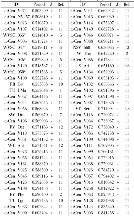
(35) 2. RR LYRAE LIGHT CURVES. 18. lower amplitudes and relatively high scatter of near-IR photometry present a challenge for this technique: in time series with a limited amount of measurements, there are not enough data to accurately determine the coefficients of the high-order truncated Fourier series needed to describe sharp features, such as the region of the minimum light of the light curves. Alternatively, light curve templates, such as those of Jones et al. (1996), could be used as model representations of the time-series. However, this approach has drawbacks: the Jones et al. (1996) templates only cover the K band, and the J-band light curves of fundamental-mode RR Lyrae are markedly different; with only four RRL templates, not all possible light-curve shapes are represented. Although the effect of metallicity on the absolute magnitudes is slightly lessened in the near-IR compared to the optical (e.g., Bono et al. 2003; Catelan et al. 2004), knowledge of individual RRL metallicities can still provide valuable insight into the star formation histories of the oldest populations of the Milky Way in parts not accessible by optical spectroscopy and/or photometry. Relationships between the light-curve shape, period, and the iron abundance [Fe/H], such as the widely used relation of Jurcsik and Kovács (1996), provide a convenient estimate in the optical regime. Despite their obvious usefulness, no such relation has been established so far in the near-IR bands. Table 2.1: Collection of RR Lyrae near-IR photometric observations. IDa AV Peg V445 Oph W Crt AR Per SW And RR Leo ω Cen V112 BB Pup ω Cen V130 WVSC 054d. Periodb 0.390375 0.397020 0.412012 0.425549 0.442262 0.452390 0.474359 0.480532 0.493250 0.501267. Jc Ref. + 10 + 4 + 12 + 10 + 1,9,10 + 10 + 11 + 12 - 11 + 5. IDa Periodb Jc Ref. ω Cen NV458 0.620326 + 11 ω Cen V032 0.620347 - 11 ω Cen V018 0.621689 + 11 ω Cen V096 0.624527 + 11 SS Leo 0.626344 + 4 ω Cen V004 0.627320 + 11 ω Cen V115 0.630469 + 11 ω Cen V146 0.633092 - 11 ω Cen V040 0.634072 + 11 ω Cen V122 0.634929 + 11 Continued on next page.

(36) 2. RR LYRAE LIGHT CURVES Table 2.1 – Continued from previous page ID Periodb Jc Ref. IDa Periodb Jc Ref. ω Cen V074 0.503209 + 11 ω Cen V041 0.662942 + 11 ω Cen NV457 0.508619 + 11 ω Cen V013 0.669039 + 11 ω Cen V023 0.510870 + 11 ω Cen V114 0.675307 + 11 ω Cen V149 0.682728 + 11 ω Cen V107 0.514102 + 11 d WVSC 055 0.514810 + 5 ω Cen V046 0.686971 + 11 ω Cen V088 0.690211 + 11 ω Cen V005 0.515274 - 11 d WVSC 047 0.519611 + 5 NSV 660 0.636985 + 13 ω Cen V008 0.521329 + 11 W Tuc 0.642230 + 2 d WVSC 046 0.529820 + 5 ω Cen V086 0.647844 + 11 X Ari 0.651180 + 3,6 ω Cen V120 0.548537 + 11 d WVSC 050 0.551535 + 5 ω Cen V134 0.652903 + 11 ω Cen V069 0.653195 - 11 ω Cen V100 0.552745 + 11 RR Cet 0.553038 + 10 ω Cen V132 0.655656 - 11 ω Cen V102 0.691396 + 11 TU UMa 0.557648 + 1 ω Cen V067 0.564446 - 11 ω Cen V097 0.691898 + 11 ω Cen V007 0.713026 + 11 ω Cen V044 0.567545 + 11 ω Cen V056 0.568023 - 11 VY Ser 0.714094 + 4,8 ω Cen V116 0.720074 - 11 SW Dra 0.569670 + 7 ω Cen V106 0.569903 - 11 ω Cen V034 0.733967 + 11 ω Cen V172 0.738049 - 11 RV Oct 0.571163 + 12 ω Cen V113 0.573375 + 11 ω Cen V085 0.742758 + 11 ω Cen V109 0.744098 + 11 ω Cen V051 0.574152 + 11 WY Ant 0.574341 + 12 ω Cen V111 0.762905 + 11 ω Cen V073 0.575215 + 11 ω Cen V099 0.766181 - 11 ω Cen V055 0.581724 + 11 ω Cen V054 0.772915 + 11 ω Cen V181 0.588370 + 11 ω Cen V038 0.779061 + 11 ω Cen V025 0.588500 - 11 ω Cen V026 0.784720 + 11 ω Cen V045 0.589116 + 11 ω Cen V057 0.794402 + 11 ω Cen V125 0.592888 + 11 ω Cen V015 0.810642 + 11 ω Cen V108 0.594458 - 11 ω Cen V268 0.812922 + 11 ω Cen V063 0.825943 + 11 RV Phe 0.596400 + 2 TT Lyn 0.597436 + 10 ω Cen V128 0.834988 + 11 ω Cen V033 0.602324 + 11 ω Cen V144 0.835320 + 11 ω Cen V090 0.603404 + 11 ω Cen V003 0.841258 + 11 Continued on next page a. 19.

(37) 2. RR LYRAE LIGHT CURVES. a. 20. Table 2.1 – Continued from previous page Periodb Jc Ref. IDa Periodb 0.604650 + 11 ω Cen V411 0.844880 0.606074 + 2 ω Cen V104 0.866308 0.608276 + 11 ω Cen V091 0.895225 ω Cen V150 0.899367 0.611618 + 11 0.615559 + 11 ω Cen NV455 0.932517 ω Cen V263 1.012158 0.615680 + 11 0.619770 + 11. ID Jc Ref. ω Cen V049 + 11 UU Cet + 11 ω Cen V079 + 11 + 11 ω Cen V118 ω Cen V020 + 11 + 11 ω Cen V027 ω Cen V062 Notes: a Unique identifier of the variable. b Period in days. c Flag whether the J band data are present and utilized in Sect 2.2.4. d The variables WVSC 054, 055, 047, 046 and 050 are V83, V116, V108, V55 and V40, respectively, from the globular cluster Messier 3 (Clement et al. 2001; Ferreira Lopes et al. 2015). References (photometric system): 1 – Barnes et al. (1992) (CIT), 2 – Cacciari et al. (1992) (ESO), 3 – Fernley et al. (1989) (AAO), 4 – Fernley et al. (1990) (SAAO), 5 – Ferreira Lopes et al. (2015) (WFCAM), 6 – Jones et al. (1987a) (CIT), 7 – Jones et al. (1987b) (CIT), 8 – Jones et al. (1988) (CIT), 9 – Jones et al. (1992) (CIT), 10 – Liu and Janes (1989) (CIT), 11 – Navarrete et al. (2015) (VISTA), 12 – Skillen et al. (1993) (SAAO), 13 – Szabó et al. (2014) (2MASS). The photometric systems are defined by González-Fernández et al. (2018, VISTA), Hodgkin et al. (2009, WFCAM), Carpenter (2001) and references therein (all other systems).. In this Chapter, special attention is paid to the particular properties of light curves produced by the VVV survey. Several new methods are introduced, driven by the desire of making maximum use of the RRLs in the VVV survey, for the analysis of variable stars in general, and for the near-IR light curves of RRLs in particular. Utilizing a high-quality RRL.

(38) 2. RR LYRAE LIGHT CURVES. 21. sample collected from the available literature (Section 2.2.1), principal component analysis (PCA) is applied to the KS -band light curves with the aim of decreasing the number of parameters parameters required to accurately describe the various light-curve shapes of RRL stars in this band (Section 2.2). It is demonstrated that the J-band light curve shape can also be approximated, utilizing the KS -band principal component amplitudes, allowing the determination of the J-band average magnitudes, even from a single observation (Section 2.2.4). Utilizing the first few principal components as basis vectors, a robust non-linear fitting technique is developed (Section 2.3). Finally, it is demonstrated, on a selected sample of OGLE-IV RRLs, that the light-curve shapes of RRLs in the KS band, together with the pulsation period, can be used to estimate their metallicities, similarly to their optical light curves (Section 2.4). The methods developed here are utilized in Chapter 3 for the characterization of the RRL population of the VVV disk fields.. 2.2 Model representation of near-IR RRab light-curves Due to its widespread use and intuitive nature, PCA has been elected as the analysis method for the near-IR RRL light curves. PCA is a widely used dimensionality reduction procedure to transform an original set of variables by an orthogonal transformation into a new set of linearly uncorrelated variables called principal components (PCs). Generally, the first few PCs contain most of the variation in the original data. The procedure was first described more than a century ago by Pearson (1901), and then rediscovered and named by Hotelling (1933). PCA has two main uses for data analysis: (1) reducing the number of dimensions of a data set by keeping only the most significant PCs and (2) identifying hidden trends in the data. As astronomical data sets are inherently multidimensional (e.g., images, spectra, individual element abundances of stars, etc.), PCA has been adopted for both purposes by the astronomical community. Among the myriad applications of PCA in astronomy are: spectral classification of galaxies (Galaz and de Lapparent 1998), stars (Singh et al. 1998), and quasars (Yip et al. 2004); modeling systematics in light curves (Jordán et.

(39) 2. RR LYRAE LIGHT CURVES. 22. al. 2013); removal of galaxies from images with the aim of finding gravitationally lensed background galaxies (Paraficz et al. 2016); analysis of galaxy velocity curves (Kalinova et al. 2017); as well as looking for correlations between diffuse interstellar band features (Ensor et al. 2017). In the context of variable stars, the most important applications of PCA for the study of Cepheids and RR Lyrae stars were presented by Kanbur et al. (2002), Kanbur and Mariani (2004), Tanvir et al. (2005), and Bhardwaj et al. (2017b). Furthermore, a range of variable star classes were analyzed with PCA by Deb and Singh (2009), in order to evaluate PCs as a metric for light curves in large databases.. 2.2.1 The light-curve training set High-quality RRL KS and J band photometry was collected from the available literature for 101 RRLs. Table 2.1 summarizes this (training) data set. The available data can be categorized into three main types: near-IR photometry taken with the aim of performing Baade-Wesselink analysis of RRLs (Barnes et al. 1992; Cacciari et al. 1992; Fernley et al. 1989; Fernley et al. 1990; Jones et al. 1987a, 1987b, 1988, 1992; Liu and Janes 1989; Skillen et al. 1993); serendipitous observations of RRLs in the 2MASS (Szabó et al. 2014) and WFCAM (Ferreira Lopes et al. 2015) calibration fields; and the extensive J and KS variability study of ω Centauri by Navarrete et al. (2015). There are other sources of near-IR time-series photometry available in the literature for RRLs (see, e.g., Angeloni et al. 2014), but only photometry where the phase coverage and quality of the observations are adequate for the accurate determination of the near-IR light-curve shapes, at least in the KS band, are utilized here. Examining the data set presented in Table 2.1 reveals that the variables in the field of ω Centauri (Navarrete et al. 2015) dominate the sample. Although this could introduce a heavy bias towards a particular metallicity, this is minimized by the fact that ω Cen contains multiple stellar populations (e.g., Valcarce and Catelan 2011; Gratton et al. 2012; and references therein), and at least two populations with metallicities [Fe/H] ∼ −1.2 and ∼ −1.7.

(40) 2. RR LYRAE LIGHT CURVES. 23. contribute to the RRL sample (Sollima et al. 2006, and references therein). The variables utilized from the photometry of Ferreira Lopes et al. (2015) are all members of the globular cluster M3, with a metallicity of ∼ −1.5 (Carretta et al. 2009). Furthermore, the field RRLs have a wide metallicity distribution, therefore this sample covers most of the possible metallicity range of RRL variables. The period distribution of the sample also covers most of the possible period range of ab-type RRLs, from 0.39 to 1.01 days. While very metal rich RRLs can have periods as short as about 0.35 days, their optical light-curve shapes are not drastically different from those with periods around 0.4 days. Therefore, it can be surmised that the present data set can be considered representative of RRLs and their light-curve shapes.. 2.2.2 Data preparation Before PCA can be applied to the data set presented in Section 2.2.1, the phase-folded light-curve shapes must be described and resampled onto a regular grid. As mentioned before, it can be hard to accurately represent the near-IR RRL light curves as a Fourier series. Furthermore, the light curves have vastly different numbers of data points: NSV 660 has almost 3000, while for the RRL found in ω Centauri, Navarrete et al. (2015) only acquired a total of 100 and 42 epochs in the KS and J bands, respectively. As an alternative to a global Fourier-series based fit, folded light curves can also be described utilizing techniques based on local fitting techniques. An example of this can be found in the work of Reyner et al. (2010), where bicubic splines were utilized to fit RR Lyrae light curves. Here an alternative method is presented, based on the linear sums of a series of basis functions. Such basis functions could be, for example, Gaussians, which can be aligned to the phased light-curve points with ordinary least squares (OLS) regression. For the problem of fitting RRL light curves accurately, the Gaussian sum fitting example of Fig. 8.4 of Ivezić et al. (2014) has been adopted, for both the KS and J-band RRL light curves. As RRL light curves are strictly periodic, Gaussians have been replaced with their periodic analogue, the.

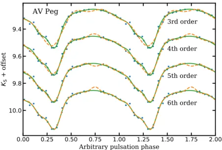
(41) 2. RR LYRAE LIGHT CURVES. KS. 9.2. 24. AV Peg. 13.0. Cen V122. 9.4 13.2 9.6. J. 13.4 9.8. KS. 13.2. 13.6. Cen V112. 13.0. 13.4. 13.2. 13.6. J. 13.4. 13.8. KS. 13.0. Cen V097. 13.6. Cen V051. 12.8. 13.2. Cen V015. 13.0. 13.4. J. 13.2. 13.6 0.0 0.2 0.4 0.6 0.8 1.0 1.2 1.4 1.6 1.8 2.0 Arbitrary pulsation phase. 13.4 0.0 0.2 0.4 0.6 0.8 1.0 1.2 1.4 1.6 1.8 2.0 Arbitrary pulsation phase. Figure 2.1: Typical folded KS (top, blue points) and J-band (bottom, orange points) light curves of the RRL sample. Each light curve is modeled with a sum of periodic Gaussian (von Mises) basis functions (Eq. 2.1), following Eq. 2.2. LASSO regularization results in most periodic Gaussians having zero amplitudes. The individual periodic Gaussian functions with non-zero amplitudes are illustrated by the faint grey lines for each band and variable. The green and purple curves illustrate the light curve fit (sum of the periodic Gaussians) in the KS and J bands, respectively.. circular normal (also called Von Mises) distributions of the form: f (x) =. eκ cos(x−µ) , 2πI0 (κ). (2.1). where µ is the measure of location (analogous to the mean of the Gaussian distribution), κ is the measure of concentration (where 1/κ is analogous to the variance, σ2 of a Gaussian), and I0 (κ) is the modified Bessel function of order 0. To model the light-curve shapes, the sum of.

(42) 2. RR LYRAE LIGHT CURVES. 25. 100 of these basis functions has been defined, distributed evenly between phases 0 and 1: LC = m +. 99 X i=0. eκ cos[2π(x− 100 )] Ai , 2πI0 (κ) i. (2.2). where Ai are the individual amplitudes of the circular normal distributions, and m is the intercept of the fit. Although OLS could be used to find the amplitudes of Eq. 2.2, most of the light curves have less than 100 points available, leading to an underdetermined problem. In such a case, regularization can be introduced to penalize the magnitude of independent parameters (in this case the amplitudes Ai ), by modifying the loss function. This is achieved by utilizing the least absolute shrinkage and selection operator (LASSO or L1 regularization, Tibshirani 1996). LASSO adds the sum of absolute values of the regression coefficients multiplied by a regularization parameter α to the loss function. While utilizing LASSO, generally most coefficients end up being zero1 . In order to implement this fitting procedure, linear regression routines of scikit-learn (Pedregosa et al. 2011) were utilized to fit the folded KS and J light curves of each RRL with the model presented by Eq. 2.2, utilizing LASSO regularization. This fit has two arbitrary hyperparameters: κ and α. Both cross-validation (leave-one-out for stars with few light-curve points, N-fold otherwise) and manual inspection of the resulting light curve fits were utilized to determine the optimal values of these parameters. High values for the concentration parameter κ (analogous to a small σ2 in the case of a simple Gaussian) grants the model the ability to fit sharp features, such as the rising branches of certain variables. However, it can also cause an overfit in phase ranges with few points. Conversely, at low values of κ the model cannot fit sharp features. It has been found that a numerical value of κ = 6 is optimal for the model for both the KS and J-band light curves of RRLs. Cross-validation and inspection of fits with different values of the regularization parameter α resulted in a range 1. Another popular choice for these kinds of problems is the Tikhonov regularization, also known as. L2 regularization or Ridge regression, where the sum of the squares of the fit coefficients times α is added to the loss function. In contrast to LASSO, Ridge regression does not result in sparse solutions (i.e., most parameters do not end up being zero), making the results of the fit harder to interpret..

(43) 2. RR LYRAE LIGHT CURVES. 26. AV Peg. 3rd order. KS + offset. 9.4. 4th order. 9.6. 5th order. 9.8. 6th order. 10.0 0.00. 0.25. 0.50. 0.75 1.00 1.25 1.50 Arbitrary pulsation phase. 1.75. 2.00. Figure 2.2: Comparison between the circular normal distribution basis fits (Eq. 2.2, continuous lines) and Fourier series of different orders (dashed lines).. of different optimal values for different stars, typically in the range between 10−4 and 10−5 . As visual inspection did not reveal significant differences when changing the regularization parameter between these two values, an intermediate value of 10−4.5 is adopted for all of the stars. Figure 2.1 illustrates the quality of the light curves and their fits. During the fitting process, some outlying points have been removed manually and the periods of some variables have been revised, when tension existed between different photometric sources. Table 2.1 contains the revised periods for all variables. Figure 2.2 compares the fits with Fourier series of different orders. As can be seen, this method provides a better representation for variables with light-curve gaps. The utilized light curves had been obtained in a variety of photometric systems, as detailed in Table 2.1. Therefore, the resulting light curve fits were all transformed to the photometric system of VISTA, in every pulsation phase. For variables not in the VISTA, WFCAM, or 2MASS systems, first they were transformed to the system of 2MASS utilizing the updated.

(44) 2. RR LYRAE LIGHT CURVES. 27 0.3. 1.0 0.5. Relative J magnitude. Normalized KS light curves. 1.5. 0.0 0.5 1.0 1.5 2.0 2.50.0. 0.2. 0.4 0.6 Pulsation phase. 0.8. 1.0. 0.2 0.1 0.0 0.1 0.2 0.3 0.0. 0.2. 0.4 0.6 Pulsation phase. 0.8. 1.0. Figure 2.3: Left: The KS -band normalized, folded and minima-aligned RR Lyrae light curves of the training set. Right: The J-band folded and minima aligned RR Lyrae light curves.. transformation formulae2 of Carpenter (2001). Then the 2MASS and WFCAM photometry was transformed to the VISTA system with the help of the CASU version 1.4 transformations given by the Cambridge Astronomical Survey Unit3 .. 2.2.3 Application of PCA to the KS -band light curves In order to apply PCA, the light curve fits are sampled on a grid of 100 phase points, evenly distributed from 0.0 to 0.99. In the analysis of pulsating variables, it is customary to set the light curve maxima at phase 0.0; however, inspecting the KS -band light curve examples of Figure 2.1 reveals that the maxima of RRLs in the KS band are ill-defined: the timing of the maxima of the light curve depends heavily on the strength of the bump on the rising branch. 2 3. http://www.astro.caltech.edu/~jmc/2mass/v3/transformations/ http://casu.ast.cam.ac.uk/surveys-projects/vista/technical/. photometric-properties The transformations between the VISTA and WFCAM systems were carried out using the relations updated on July 30, 2014. Updated transformations were provided by González-Fernández et al. (2018). The changes in the resulting transformed magnitudes were revised, and were found to be less than 0.005 mag. Since, in addition, this only affects the five stars from Ferreira Lopes et al. (2015), none of the results in this chapter are significantly affected by the choice of transformation equations between these two systems..

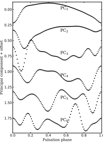
(45) 2. RR LYRAE LIGHT CURVES. 28. Therefore, as an alternative, the light curves were aligned by the much sharper feature of the light curve minima (similarly to the case of eclipsing binaries). In most applications of PCA, the sample values (the magnitudes in this case) are usually normalized to a mean of 0 and scatter of 1 along each dimension (phase) after subtracting the mean value along each dimension (phase). As the goal here is to describe the light-curve shapes of RRLs in the KS band as a linear combination of PCs, it has been found that better results are obtained by not subtracting the mean in each dimension. Furthermore, in this case, each light curve is normalized independently to have a mean of 0 and scatter of 1. These aligned, normalized input light curves can be seen in the left panel of Figure 2.3. PCA was carried out by utilizing a related transformation called singular value decomposition (see, e.g. Chapter 7.3.1 of Ivezić et al. 2014), adopted from the PCA module of scikit-learn (Pedregosa et al. 2011)4 . Figure 2.4 shows the first six PCs, according to the PCA decomposition of the RRL KS -band light curve sample. As the light curves were chosen not to be mean subtracted and normalized in each dimension (phase), the first PC contains the average light-curve shape of the normalized light curves. As the original light curves (presented in the left panel of Figure 2.3) can be reconstructed as a linear combination of the PCs, the role of further components in the description of individual light curves can be easily understood. For example, the second component modifies the average light curve (the first PC), so that the bump at the end of the rising branch (around phase 0.15) can become more or less pronounced, while the third component is important to reproduce the double-peaked light curves displayed by some of the variables. The power of the PCA lies in the fact that generally the first few PCs, together with their amplitudes, are sufficient to describe the original input data with high accuracy, and the rest of the PCs can be discarded, greatly reducing the number of parameters. The number of significant PCs can be decided by examining the fraction of the variance explained by the components. As each light curve was normalized individually instead of normalizing the 4. The PCA module present in scikit-learn automatically subtracts the mean along each data dimension,. hence the need for the modification of the original algorithm..

(46) 2. RR LYRAE LIGHT CURVES. 29. PC1. 0.00. Principal component + offset. 0.25. PC2. 0.50. PC3. 0.75 1.00. PC4. 1.25. PC5. 1.50 1.75 0.0. PC6 0.2. 0.4 0.6 Pulsation phase. 0.8. 1.0. Figure 2.4: The first six principal components of the decomposition of the KS -band RRL light curves.. magnitudes along each dimension (phase), obviously the first PC dominates, with 95.6 percent of the explained variance. The rest of the PCs explain 3.68, 0.14, 0.01, 0.007, etc. percent of the total variance, or 88.8, 3.4, 2.3, 1.7, etc. percent of the residual variance, when the variance explained by the first PC is subtracted from the total variance. Based on these values, as well as inspection of the effect that the omission of different PCs have on the reconstructed light curves, it has been deemed that the first four PCs are sufficient for describing the KS -band light-curve shapes of RRab stars. The PCA method has been applied to the normalized light curves of the sample of variables, in order to emphasize the light-curve shape differences among RRLs in the KS band,.

(47) 2. RR LYRAE LIGHT CURVES. 30. instead of the different pulsation amplitudes that each variable has. Consequently, the individual amplitudes (also called eigenvalues) of the first four PCs, u1 j , u2 j , u3 j and u4 j , where j = 1..101 is the index of the variables, are insufficient to reconstruct the original light curves, as they have lost the amplitude information due to the normalization of the individual light curve variances. However, by multiplying these amplitudes with the normalization constants applied to the light curves (or, alternatively, by utilizing OLS to directly align the PCs to the light curves), a modified set of PC amplitudes U1 j , U2 j , U3 j and U4 j are created for each star in the sample. The sum of the PCs multiplied with these amplitudes recover the original light-curve shapes (and amplitudes) with high accuracy. The distribution of the amplitudes Ui j is illustrated in Figure 2.5. The shapes of the light curves of RRLs, represented by the amplitudes of these first few PCs, potentially contain information on the physical properties of the variables themselves, when the pulsation periods of the stars are taken into account. The first amplitude, U1 (from now on, the j index is omitted for simplicity) can be viewed as an analogue to the total amplitude in amplitude-period (also called Bailey) diagrams. As described before, additional PCs with non-zero amplitudes modify the average light-curve shape. Therefore, by inspecting Figure 2.5, it is immediately obvious that, at a given period, the amplitudes U1 and U2 separate mainly the stars into two sequences, which can be associated with the Oosterhoff type I and II groups of variables (Oo; Oosterhoff 1939; see Catelan and Smith 2015, for a recent review and references). As these groups at least partly correlate with metallicity, such a clear separation hints at the effect metallicity has on the near-IR light curve shapes of RRL variables, similarly to their visual light curves. The possibility of estimating the metallicity of individual RRLs based on their KS -band light curves, as described by their PC amplitudes Ui , is going to be explored in Section 2.4..

(48) U2. U1. 2. RR LYRAE LIGHT CURVES. 1.1 1.0 0.9 0.8 0.7 0.6 0.5 0.4 0.3 0.2 0.1 0.0 0.1 0.2 0.3 0.10. 31. Cen Cen, no J Messier 3 Field 0.4. 0.5. 0.6. 0.7. 0.8. 0.9. 1.0. 0.4. 0.5. 0.6. 0.7. 0.8. 0.9. 1.0. 0.4. 0.5. 0.6. 0.7. 0.8. 0.9. 1.0. 0.4. 0.5. 0.6 0.7 0.8 Pulsation period [d]. 0.9. 1.0. U3. 0.05 0.00 0.05 0.10 0.10. U4. 0.05 0.00 0.05 0.10. Figure 2.5: Amplitudes Ui of the PCs of the training sample. Circles and squares denote RRLs from the ω Centauri photometry of Navarrete et al. (2015) and other sources, respectively. Empty squares denote RRLs in Messier 3 from the photometry of Ferreira Lopes et al. (2015), while empty circles denote variables not considered for the approximation of the J-band light-curve shapes in Section 2.2.4..

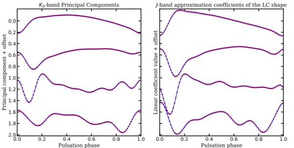
(49) 2. RR LYRAE LIGHT CURVES. 32. 2.2.4 Approximation of the J-band light curve shape The light-curve shapes and amplitudes of pulsating variables vary among bandpasses, due to the difference in the relative contribution of the change of radius and photospheric temperature during the pulsation cycle to the emitted flux at different wavelengths (Catelan and Smith 2015, and references therein). Comparing the KS and J-band light curves in Figure 2.1 clearly demonstrates this. During the course of the VVV survey, each field has been observed only a few times in the J band. In order to determine accurate mean J magnitudes for the RRLs, it is necessary to describe the light-curve shapes of the stars in the J band, i.e., the deviation of the Jband magnitude from its average in each phase of the pulsation cycle. Usually the difference between the light-curve shapes is ignored, and the KS -band light-curve shape is used to estimate the average J-band magnitude. However, this method, depending on the light-curve phases of the observations, introduces additional scatter in the derived magnitudes. As the PC amplitudes Ui provide a concise description of the KS -band light-curve shapes, it can be evaluated whether the J-band light-curve shapes can be approximated with their use. Besides these amplitudes, the effect of the period is also considered as a possible additional parameter, in order to assess its possible effect on the J-band light curves of variables that otherwise possess the same light-curve shapes in the KS band. Fourteen of the variables marked in Table 2.1, coming from the ω Centauri sample of Navarrete et al. (2015), have problematic J-band photometry, mostly due to inadequate phase coverage, therefore they are omitted, and the remaining 87 stars are analyzed. These J-band light curves are first sampled in the same 100 phase points as has been done for the KS -band light curves in Section 2.2.3, where phase 0.0 is the phase of the KS -band light-curve minimum for each of the variables5 . These curves are aligned to have a mean of 0, but in contrast to the PCA analysis of the KS -band light curves, they are not normalized in amplitude. 5. All of the stars have simultaneous J and KS -band photometry, therefore the possibility of systematic. differences between the real pulsation phases between these two bands in negligible..