TítuloOn the resolution of the navier stokes equations by the finite element method using a sups stabilization technique application to some wastewater treatmen problems
255
0
0
Texto completo
(2) T. 7. UNIVERSIDAD DE LA CORUÑA DEPARTAMENTO DE MÉTODOS MATEMÁTICOS Y DE REPRESENTACIÓN. PROGRAMA DE DOCTORADO EN INGENIERÍA CIVIL. ON THE RESOLUTION OF THE NAVIER-STOKES EQUATIONS BY THE FINITE ELEMENT METHOD USING A SUPG STABILIZATION TECHNIQUE. Application to some wastewater treatment problems. by Pablo Rodriguez-Vellando Fernández-Carvajal. supervised by: Jerónimo Puertas Agudo Ignasi Colominas Ezponda. Doctoral Thesis La Coruña, March 2001.
(3) a mi padre.
(4) CONTENTS. •. ACKNOWLEDGEMENTS. •. NOTATION. •. INTRODUCCIÓN, RESUMEN Y CONCLUSIONES ..........................................1. •. CHAPTER 1. INTRODUCTION AND GOVERNING EQUATIONS ..............15 1.1. The physical problem. 15. 1.2. Numerical resolution of the flow problem. 17. 1.3. Finite element resolution of the flow problem. 18. 1.4. Governing equations ,. 23. 1.4.1. Conservation of mass ^. •. 25. 1.4.2. Conservation of momentum. ^. 27. 1.5. The 2D laminar Navier-Stokes equations. 32. 1.6. The Shallow Water equations. 34. 1.6.1. Continuity equation. 36. 1.6.2. Dynamic equation. 37. 1.6.3. Treatment of the viscosiry effects. 40. CHAPTER 2. FINTTE ELEMENT RESOLUTION OF THE VISCOUS INCOMPRESSIBLE FLOW ..................................................................................49 2.1. Finite element formulation of the viscous incompressible flow. 49. 2.1.1. The weighted residuals method. 50. 2.1.2. Obtaining of a weak form. 52. 2.1.3. Discretization. 54. 2.2. Mixed formulation. 61. 2.3. Penalty formulation. 63. 2.3.1. Introduction. 63. 2.3.2. The variational Lagrange-multipliers technique. 64. 2.3.3. The penalty approach to the Navier-Stokes equations. 68. 2. 4. Segregated formulation 2.4.1. Introduction. ^ ^. 2.4.2. The segregated approach to the Navier-Stokes equations. 72 72 73.
(5) 2.5. Shallow Water formulation. 79. 2.5.1. The equations to be solved. 79. 2.5.2. Numerical procedure: the star depths and star gradients of depth. 81. 2.6.- The SUPG stabilization technique 2.6.1. Introduction. 84 84. 2.6.2. The upwind firvite difference stabilization technique for the advectiondiffusion equation. 86. 2.6.3. The finite element SUPG stabilization technique for the advectiondiffusion equation. 89. 2.6.4. The finite element SUPG stabilization technique for the mixed NavierStokes formulation. 92. 2.6.5. The finite element SUPG stabilization technique for the penalty NavierStokes formulation. 94. 2.6.6. The finite element SUPG stabilization technique for the segregated Navier-Stokes formulation. 95. 2.6.7. The finite element SUPG stabilization technique for the mixed ShallowWater formulation 2.7. Resolution of the system of equations. 97 97. 2.7.1. Transforming the non-linear system into a linear system of equations. 98. 2.7.2. Transforming the differential system into an algebraic one. 99. 2.7.3. Detailed matrix expression of the mixed and penalty formulation. 101. 2.7.4. Detailed matrix expression of the segregated formulation _. 102. 2.7.5. Detailed matrix expression of the mixed Shallow Water formulation 104. •. 2.7.6. The direct solver with skyline storing. 105. 2.7.7. The iterative solvers used in connection with sparse storing. 109. 2.7.8. The iterative solver: the Biconjugate Gradient Method. 112. CHAPTER 3. VALIDATION OF THE MIXED, PENALTY AND SEGREGATED ALGORITHMS MAKING USE OF THE CAVITY FLOW ^ BENCHMARK PROBLEM .................................................................................118 3.1. The Driven Cavity Flow benchmark problem. 118. 3.2. Resolution of the Cavity Flow by the mixed approach. 121. 3.3. Resolution of the Cavity Flow by the penalty approach. 132.
(6) •. 3.4. Resolution of the Cavity Flow by the segregated approach. 137. 3.5. Conclusions. 142. CHAPTER 4. FLOW OVER A BACKWARD FACING STEP. CHECKING THE ALGORITHM WITH EXPERIMENTAL RESULTS .............................143. •. 4.1. Introduction. 143. 4.2. The flow over the backward facing step benchmark problem. 143. 4.3. Results. 144. 4.4. Conclusions. 156. CHAPTER 5. CONSIDERATION OF THE FRICTION SLOPE AND UNSTEADY DEVELOPMENT OF THE FLOW. FLOW IN A WATER DISTRIBUTION CHAIVIBER ..............................................................................157. •. 5.1. Introduction. 157. 5.2. Resolution of the flow for several Reynolds numbers. 158. 5.3. Consideration of the friction slope. 164. 5.4. Unsteady development of the flow. 167. CHAPTER 6. THE 2D LAMINAR NAVIER-STOKES vs THE SHALLOW WATER FORMULATIONS ................................................................................172 6.1. Introduction 6.2. F1ow for natural and adverse flow conditions. ^. 172 173. 6.3. Flow for an adverse steep slope. Navier-Stokes vs Shallow Water equations 177 •. CHAPTER 7. APPLICATION TO SOME WASTEWATER TREATMENT. PROBLEIVIS ...........................................................................................................180 7.1. Flow in a clarification basin. •. 181. 7.1.1. Rectangular clarifier. 182. 7.1.2. Circular clarifier. 187. 7.2. Flów in a lamellar `LUPA' clarifier. 192. 7.3. Flow in a maze floculator. 198. 7.4. Conclusions. 202. CHAPTER 8. CONCLUSIONS AND FURTHER DEVELOPMENTS...........204 8.1. Conclusions. 204. 8.2. Further developments. 205.
(7) •. •. APPENDIX. ............................ ......................................... .......................................208 A1. The finite element local reference system. 208. A2. Numerical integration. 215. REFERENCES ......................................................................................................219. `^.,.
(8) ACKNOWLEDGEMENTS The author wants to express his gratitude to all the people and institutions taking part in the working out of this doctoral thesis, without whom it would not have been possible to conclude this work. First, I would like to give my thanks to the School of Civil engineering of La Coruña and the University itself, where all this work has taken place, not only as an institution, but also to the particular individuals who working in it, already know of my gratitude. I would specially like to mention the help given by the people in the Departamento de Métodos Matemáticos y de Representación, regarding the numerical aspects of this work. I would also like to thank the technical support on wastewater engineering provided by Joaquín Suárez and José Cril de Bernabé, and the help given by my PhD colleagues Juanjo Bonillo and Jaime Fe. Not to mention the support provided by the codirectors of this doctoral thesis Jerónimo Puertas and Ignasi Colominas, without the help of whom this work would not have been brought to fruition. Thanks to Rodolfo Bermejo from the Universidad Politécnica de Madrid for his guidelines in the beginning of this work. I would also like to express my gratitude to the company Endesa (As Pontes) for its financial support. Many thanks to all of them. To the friends and family (some of them already included in the upper paragraph), who helped me to keep my unsteady state of mind and mood for the preparation of this doctoral thesis, I would rather thank their priceless aid in a different forum, and I hope I will.. This work has also benefited from the hydraulic projects: - Criterios para el diseño de escalas de peces de hendidura vertical (HID99-0297, U00-XII/02), funded by the CICYT (Ministerio de Educación y Cultura). - Optimización de circuitos hidrodinámicos y d^ los procesos en instalaciones de tratamiento físico-químico de agua. Aplicación a la planta de efluentes químicos de As Pontes (1 FD 1997-0053/HID 1, XU98-X/O1), funded by the FEDER (EC). And also from the projects of the Dep. de Métodos Matemáticós y Rep.: - Desarrollo de un sistema global de cálculo avanzado y diseño de redes de tierra de subestaciones eléctricas (1 FD97-0108, XU98-X/O1), funded by the FEDER (EC).. ..
(9) - Desarrollo de un entorno de diseño óptimo asistido por ordenador de torres y líneas de alta tensión (TIC98-0290, U99-31/O1), funded by the CICYT (Ministerio de Educación y Cultura)..
(10) NOTATION. The indicial notation will be used throughout the text, together with the usual summation convention for repeated indices. The indices after commas will stand for derivatives with respect to the variables specified in the index. Variables in boldface refer to vectors or matrices as a whole. The international system of units (Sn will be used throughout the text except for the cases in which a different unit is of common use. The symbols included in this thesis stand for the following variables:. Latin symbols A. Reduced viscous coefficient matrix. Av. Viscous coefficient matrix. A. PBCG preconditioning matrix. B. Gradient of pressure matrix. BE. Penalty matrix. bb. Wetted perimeter of a boundary basic element. b;. Prescribed velocity. b;n. Wetted perimeter of an interior basic element. C„ (u, v^. Convective coefficient matrix. C(u, v^. Reduced convective coefficient matrix. d. Depth with respect to a system parallel to the bottom of the channel. e^;,en;. Unit vectors in the ^ and r^ directions. f. Body force vector. f,•. Body forces components. g. Gravity force. h. Depth vector. h. Depth with respect to a horizontal reference system or size of the grid. h'. Star depth. H;. Quadrature rule coefficient. ^.
(11) h^. Star gradient of depths. H k (S2}. Sobolev space of order k over the domain S2. h^ , h,^. Characteristic basic element lengths in the ^ and r^ d^ections. Hó (S2}. Subspace of H' (S2} vanishing on I',. J. Jacobian determinant of the transformation. k,^. Diffusion. k^^. Artificial diffusion. K;p. Pressure-velocity coupling coefficient. L. Lower triangular matrix. L2 (S2}. Hilbert space over the domain S2. Lo (SZ}. Subspace of L2 (S2} with zero mean over the domain SZ. m. Mass. M. Number of pressure nodes. M. Unsteady reduced coefficient matrix. M„. Unsteady coefficient matrix. ma. Momentum. n. Manning roughness coef. or outward unit vector normal to the interface. N. Number of velocity nodes. n'. Modified Manning roughness coefficient. nn. Number of nodes. ne. Number of elements. N,. Velocity shape function. p. Pressure vector. p. Pressure. ph. Discretized pressure. ^. ^. 3. SUPG contribution to the weighting function. Pk,^k. PBCG sequences of vectors. q. Weighting function. Q1Po. Bilinear velocity-constant pressure basic element.
(12) r. Inertial relaxation factor. Re. Reynolds number. Rh. Hydraulic radius. rk, P^. PBCG sequences of vectors. So. Geometric slope. Sf. Friction slope. Só (S2^. Discretized subspace belonging to Ló (S2^ over the domain S2. t. Time. t^. Traction vector. U. Upper triangular matrix. u. Velocity along the x direction. u. Velocity vector in the x direction. u;`. Discretized velocity. u;(x;,t). Velocity Mean horizontal velocities in the x direction. ^. ^. ^. R;. Pseudo-velocities in the x direction. v. Velocity along the y direction. v. Velocity vector along the y direction. V. Volume of integration. Vó (S2 ^. Discretized subspace belonging to H 1(S2^ over the domain S2. Vo. Initial volume. ^. ' Mean horizontal velocities in the y direction. ^t. Pseudo-velocity in the y direction. w. Velocity along the z direction. w;. Weighting functions. x;. Spatial directions. Z. Height of the free water surface. Zb. Height of the bottom of the channel. Zk, ^k. PBCG sequences of vectors.
(13) Greek symbols ap. Pressure relaxation parameter. au. Velocity relaxation parameter. a^,a,^. D^ectional Reynolds numbers in the ^ and r^ directions. a. Peclet number. I'. Boundary of the S2 domain. S;^. Kronecker delta. E. Penalty parameter. E,^. Eddy viscosity coefficients. ^;^. Rate of deformation. r^. Local spatial variable. r^(x, y). Perturbation function. ^,. Lagrange-multiplier. µ. Dynamic viscosity of the fluid. v. Kinematic viscosity of the fluid. ^. Local spatial variable. p. Density of the fluid. 6^^. Stress along the boundary. Tb. Shear stress acting on the water bottom. T;^. Stress. zs. Shear stress acting on the water surface. ^. Concentration. v_. Velocity vector. x;. Pressure shape function. S2. Domain of integration. S2h. Discretized domain. aV. Volume V boundary. aS2. Domain boundary. ^. ^.
(14) INTRODUCCIÓN, RESUMEN Y CONCLUSIONES. In my beginning is my end.. Tbomas S. Eliot, 1888-1965 Four Quanets, East cooker.
(15) Introducción, resumen y conclusiones. INTRODUCCIÓN, RESUMEN Y CONCLUSIONES. Las ecuaciones de Navier-Stokes, que rigen el flujo viscoso incompresible, sólo tienen solución analitica para un limitado numero de casos simplificativos. Para conseguir un procedirniento que resuelva de manera sistemática los problemas del flujo incompresible, debemos recurrir a alguna técnica numérica que nos aporte una solución aproximada de los problemas reales. El Método de los Elementos Finitos es junto con el de los Volúmenes Finitos la técnica numérica más comúnmente utilizada hasta la fecha para resolver las ecuaciones de Navier-Stokes. El Método de los Elementos Finitos fue desarrollado en un principio para el cálculo de estructuras, sin embargo la resolución del flujo viscoso incompresible requiere un tratamiento especial para resolver ciertos problemas que no aparecen en el cálculo convencional de estructuras. Estos problemas derivan de la necesidad de verificación de la ley de conservación de la masa, en una sustancia que cambia constantemente de forma, de la existencia de dos tipos distintos de incógnitas en la ecuación constitutiva (velocidad y presión), de la asimetría de la matriz de `rigidez' debido a la presencia de los términos convectivos, de la existencia de fuerzas viscósas entre partículas, de la dependencia de las variables con respecto del tiempo, etc. Algunas de estas dificultades pueden ser ignoradas si se hacen ciertas simplificaciones, que como la de Stokes ignoran los términos convectivos, o la de flujo potencial que hace caso omiso de los esfuerzos viscosos. Sin embargo, estas simplificaciones sólo nos dan una aproximación para ciertos casos sencillos de flujo. Todas estas particularidades exigen la utilización de una formulación en elementos finitos que se adapte a las características singulares de los fluidos. Los tipos de formulación usados en la resolución de las ecuaciones 2D de Navier-Stokes por el Método de los Elementos Finitos en este trabajo, han sido las formulaciones mixta, penalizada y segregada, y reciben esta denominación dependiendo de la forma en la que se tratan las incógnitas velocidad y presión por un lado, y las ecuaciones dinámica y de continuidad por otro. Estos tres tipos de algoritmos son los más comúnmente utilizados en la literatura afín, siendo estos. métodos en los que muchos autores acuerdan en. dividir las formas de resolver las ecuaciones de Navier-Stokes por el Método de los Elementos Finitos [Kim 88], [Choi 94].. I.
(16) Introducción, resumen y conclusiones. La forma más intuitiva de las tres de resolver el problema del flujo incompresible es la formulación mixta, que se basa en aplicar el método de los residuos ponderados directamente sobre las dos ecuaciones de la ley de Navier-Stokes, esto es ecuación dinámica y de continuidad.. Jn Wh (u^+u. i,i. f, )+v Jnw^^uh^dS2- 1 JnWh`pdSZ-,^- t;`W;`dI'2 -O P 2 Jqhuh,dSZ = 0 n. Una vez se ha obtenido una forma débil y la aproximación ha sido introducida en la formulación, se llega a un sistema de ZN+M ecuaciones diferenciales para el caso 2D, siendo N y M el número de nodos de interpolación de velocidades y presiones en los que se ha dividido el dominio. Las necesidades de memoria para almacenar los datos implicados como consecuencia de la utilización de una formulación de tipo mixto son muy grandes. Por otra parte, el proceso iterativo encaminado a la resolución de la convección es más directo que en los otros casos que veremos a continuación. De otro lado, los problemas de consistencia que emergen como resultado de la necesidad de verificación de la condición de divergencia-estabilidad (o también llamada condición de Ladyzhenskaya-Babuska-Brezzi en honor a sus descubridores y estudiosos), hacen que la elección de los elementos básicos en términos de los cuales el dominio de definición es dicretizado sea una cuestión de vital importancia [Babuska 71], [Brezzi 74]. La elección de un elemento básico inadecuado (como la aparentemente inofensiva utilización de una malla de igual orden para las incógnitas velocidad y presión), puede provocar la obtención de la solución trivial como única posible, dar lugar a la divergencia del proceso iterativo o provocar la aparición de oscilaciones nodo a nodo en el campo de presiones (solución también conocida como `presión en tablero de ajedrez'). Estos tipos de soluciones espurias fueron detectadas y caracterizadas por Taylor y Hood en un artículo de 1973 [Taylor 73]. Para evitar este tipo de inestabilidad, Taylor y sus colaboradores idearon un elemento básico conocido con el nombre de par de `Taylor-Hood', que cumple estrictamente la condición LBB y con el que obtuvieron buenos resultados en la resolución del flujo viscoso incompresible. Sin embargo, existen elementos básicos, como es el caso del elemento Q 1 P0, que sin cumplir estrictamente la condición de divergencia-estabilidad, han permitido obtener soluciones estables. Los. 2.
(17) Introducción, resumen y conclusiones. buenos resultados obtenidos en el presente trabajo, con el elemento básico de tipo Q1P0 (velocidad bilineal, presión constante), que ni siquiera ha mostrado dar lugar a los campos de presión en tablero de ajedrez que aparecen en los trabajo ^ de otros autores (ver por ejemplo [Fortin 77] y[Brooks 82]), nos ha llevado a utilizar este elemento básico en todos nuestros cálculos con óptimos resultados. La formulación penalizada, también utilizada en este trabajo permite gracias a la utilización de un apazato matemático basado en el cálculo variacional y recuperado por Zienkiewicz en 1974 para el Método de los Elementos Finitos, la reducción en el número de ecuaciones presentes en el sistema algebraico a una cantidad igual a dos veces el número de incógnitas de velocidad del dominio [Zienkiewicz 74]. El trabajo de Zienkiewicz seria continuado en [Teman 77], [Bercovier 79], [Hughes 79] y[Brooks 82]. El campo de presiones en los algoritmos penalizados es obtenido a posteriori como un valor de postproceso y por lo tanto no consume recursos a la hora de la resolución del sistema. La formulación podría presentarse de forma simplificada como: h h h h h h h (^ h k jw;h (u;^ +u^u;,^ - f;)+v JQw;,^u;,^dS2+ J^1 u;^w;^dS2-. ^lL2t; w; dr2 =0; Q. h. 1. p=--u^, ^. Qh. Esta formulación, elimina la ecuación de continuidad del sistema a resolver, pero a cambio introduce un parámetro numérico llamado de penalización ( E) próximo a cero, cuya elección va a ser muy importante en la obtención de una convergencia adecuada. La elección de un parámetro de penalización demasiado pequeño va a provocaz que el término de penalización sea varios órdenes de magnitud mayor que el término viscoso. Una correcta elección de E implicará un equilibrio entre un número. v. suficientemente grande como para que el tamaño de una unidad básica de memoria del ordenador sea capaz de almacenaz la información de los términos viscoso (pequeño) y penalizado (grande) en el misma variable; y un número suficientemente próximo a cero como para permitir la correcta convergencia del problema. Por otra parte, en las formulaciones penalizadas aparece un problema análogo al que se nos presentaba en la formulación mixta cuando se usaba una interpolación del mismo orden para las incógnitas velocidad y presión. Cuando en la formulación de penalización los términos implicados son integrados con leyes de cuadratura del mismo orden de error, podemos encontrarnos con que la única solución posible del sistema es la trivial. Este fallo en la resolución del flujo puede evitarse mediante lo que conocemos. 3.
(18) Introducción, resu^n y conclusiones. como una `integración reducida selectiva', que consiste en integrar las matrices elementales de penalización con una ley de cuadratura de orden inferior a la usada en el resto de los térrr^nos. De esta forma, el término de penalización no es exacto, la matriz asociada correspondiente deja de ser regular, y con ello se `desbloquea' la obtención de la solución trivial. Por último, la formulación segregada consiste en una resolución secuencial de las variables presión y velocidad, a través de la resolución de dos sistemas diferenciados para la ecuación dinámica y de continuidad, que se obtienen gracias a la aplicación del método de los residuos ponderados. El método fue desarrollado en un principio para las formulaciones en diferencias finitas y volúmenes finitos [Patankar 80], [Ferzinger 96]. Debido a sus buenos resultados fue extendido en la década de los 70 al Método de los Elementos Finitos. Desde entonces muchos autores han realizado aportaciones en este sentido, entre las cuales se pueden destacar las de [Scheneider 78], [Benim 86], [Rice 86], [Shaw 91] y[Haroutunian 93] entre otros. La formulación aquí utilizada será una variante de la empleada por Rice sobre la que han trabajado muchos otros autores como [Zij191], [Choi 97], [du Toit 98]. El fundamento de esta formulación parte de aplicar el método de los residuos ponderados a las ecuaciones dinámica y de continuidad, para obtener:. Sistema dinámico: t;'W;`dI'2 ^iS2+V^Wh^rj uh d^2= JWht fi d^2- 1 JQw.``p^dS2+^, jW;`^lth^ +Uhu;` J .j tr! Q n p ^ 2 Sistema de continuidad: jwhju^dS2- jw;`u^n ^ dl'2 =0 nh r2. v. En la primera iteración se hace una suposición para el campo de presiones, en función de la cual de obtiene un resultado para el campo de velocidades en el sistema dinán^co, que una vez obtenido es realimentado en el sistema de continuidad. La conexión entre ambos sistemas se hace mediante la definición de un conjunto de variables Q; y tri , conocidas con el nombre de pseudovelocidades y definidas de la forma:. ai = p^ Oii. T^ = 1. -^jdi;u; +fsi ixj. 8ii. 4. -^gijvj +fy; ixj.
(19) Introducción, resumen y conclusiones. donde g;^ es la matriz de cceficientes del sistema dinámico, que según esto se puede expresar como: 1 ui =p O ii. aNj. p -^,Oi;u; + ^si -JS2w^ ;xi. r v; _ ^ -^jOijvj + fyi O ii. jxi. J. ^w;. ^n. aX pj ^L. aN . ' pj dS2 ^. donde la relación entre las velocidades y las pseudovelocidades, y los cceficientes de conexión K;p pueden escribirse matemáticamente como: %li ,^ ^r; _ KiP. aN.^ ax. p! ;. aN. vi = v^ - K;° ^ p j;. K;p = 1 f^ W; dS2 S ii. Una vez se han resuelto ambos sistemas, las velocidades son corregidas y el proceso se repite hasta alcanzar la convergencia. Para que este algoritmo llegue a converger, será necesario introducir una relajación en las variables incógnita, función de un parámetro que será obtenido por tanteo numérico. La formulación segregada, aparte de permitir la utilización de una misma malla en la interpolación de las variables velocidad y presión sin provocar problemas de consistencia, consigue que el tamaño de los sistemas a resolver sea reducido al número de nodos de velocidad o presión, con lo que la matriz de coeficientes es de menor tamaño. Además, por la propia definición de la formulación, la matriz de cceficientes asociada a los sistemas se puede expresar como una matriz de ancho de banda estrecho, cuando se lleva a cabo una correcta renumeración de los nodos. Los algoritmos hasta ahora expuestos resuelven las ecuaciones de Navier-Stokes en dos dimensiones, de forma que la tercera dimensión del espacio es totalmente ignorada. La formulación de Aguas Someras es utilizada como una manera de incluir la tercera dimensión, para los casos en los que el calado del flujo es pequeño en comparación con la dimensión horizontal. Este algoritmo hace la suposición de que la dirección principal del flujo es la horizontal, y sólo flujos despreciables tienen lugar en planos verticales. Asimismo, la aceleración en la dirección vertical es considerada despreciable en comparación con la gravedad, y se asume una distribución hidrostática de presiones. La simplificación de Aguas Someras supone que la distribución de las velocidades horizontales a lo largo de la dirección vertical es uniforme, y en consecuencia se lleva a cabo una integración en altura, para así considerar como. 5.
(20) Introducción, resumen y conclusiones. velocidad horizontal la media de velocidades a lo largo de la vertical. El calado y el gradiente del calado entran ahora a formar parte de la ecuación de continuidad, permitiendo así que la tercera dimensión afecte a la conservación de la masa, y que de esta forma el balance de masas no se haga en función de las dos dimensiones horizontales del flujo. Para valores suficientemente grandes del número de Reynolds, aparece en los fluidos una forma de flujo caótico y no permanente de manera intrínseca, que conocemos como turbulencia. El estado turbulento va a suponer la aparición de remolinos de muy escaso tamaño (del orden de hasta 10 µm ), y elevada frecuencia (del orden de IOKHz), con lo que la captación de estos fenómenos requeriría una malla extremadamente fina, si no se utiliza un modelo específico de turbulencia. La forma más habitual de abordar los estados turbulentos es descomponer las magnitudes implicadas en el flujo en un instante dado, en la media temporal de esas variables en un determinado intervalo, más un cierto término función del tiempo. La evaluación de la velocidad y la presión del flujo en esta forma, dará lugar a la aparición de un término adicional en las ecuaciones de Navier-Stokes, conocido como término de tensiones de Reynolds. Este término puede ser evaluado mediante un modelo específico de tuifiulencia de una o varias ecuaciones, como es el caso de los modelos de longitud de mezcla o el modelo k-^ En esta tesis no se ha considerado un modelo específico de turbulencia, ya que los casos a los que se va a aplicar no lo requieren. Sin embargo, se ha incluido una evaluación de la pendiente motriz en términos de la fórmula empírica de Manning, que si bien no permite captar los remolinos del flujo turt^ulento, si que estima las pérdidas de energía globales, que incluyen también las tensiones turbulentas. La resolución de las ecuación de aguas someras se hará según un algoritmo de tipo mixto, que por lo tanto participará de las mismas ventajas e inconvenientes expuestos para la formulación mixta 2D de Navier-Stokes. Para materializar la influencia del calado sobre la ecuación de continuidad, se definirán unos valores intermedios del calado h` y del gradiente del calado b' , evaluados según un esquema en diferencias finitas desarrollado por el autor, para así eliminar los términos con cuasino-linealidades.. 6.
(21) Introducción, resumen y conclusiones. h h h h J w;h u;hu r,; - 8(So; - S hf )^iS2 + v J^h w;,;u=,^ dS2 - g J^k w;,;h h hdS2 -^,, t;h w;h dI'2 = 0 nn . r s J qh h hu ^ +uhh^ih ^h. Aparte de los problemas de inestabilidad que surgen como consecuencia de la forma en que son tratadas las incógnitas presión y velocidad, y de la elección de los elementos básicos en función de los cuales el dominio es discretizado, otro grupo de problemas de inestabilidad numérica potencial que aparece a la hora de resolver los problemas del flujo viscoso, es el de los provocados por la forma en que el método de los residuos ponderados se aplica sobre el término de convección de la ecuación dinámica. En efecto, la forma simétrica en que la formulación de Galerkin (funciones de peso iguales a funciones prueba), trata al término convectivo no simétrico, resulta ser el origen de una fuente de inestabilidad en la obtención de la solución de las ecuaciones de Navier-Stokes. Esta inestabilidad aparece en forma de oscilaciones espurias nodo a nodo en el campo de velocidades, que en la literatura anglosajona se suelen conocer como `wiggles'. Estas oscilaciones que aparecen como consecuencia de la existencia del término de convección en las ecuaciones de Navier-Stokes, se hacen lógicamente más ostentosas cuanto mayor es el peso de la convección en el flujo, y por lo tanto son mayores cuanto más grande es el número de Reynolds. Estas oscilaciones se pueden eliminar llevando a cabo un exhaustivo refinamiento de la malla, especialmente en aquellos lugares donde existe un cambio brusco en las condiciones del flujo. Sin embargo, este refinamiento puede implicar unos costes computacionales muy altos, que depende de las condiciones particulares del flujo en cuestión y pueden convertir el. •. problema en inabordable para ciertos casos caracterizados por números de Reynolds suficientemente altos. Fue en el congreso MAFELAP de 1975, cuando Zienkiewicz planteó una forma de resolución de estos problemas del flujo incompresible mediante un algoritmo de estabilización [Zienkiewicz 76]. Como consecuencia de este encuentro, surgen trabajos [Heinrich and Huyakom 77], [Heinrich and Zienkiewicz 77], que proponen la utilización de esquemas, que llamados de Petrov-Galerkin, permiten la estabilización de la ecuación de conveción-difusión mediante la utilización de funciones de peso y de prueba distintas.. Sin embargo, cuando se intentó generalizar este procedimiento de estabilización a las ecuaciones de Navier-Stokes, se encontró que aparecían unos modos de difusión. ^.
(22) Introducción, resumen y conclusiones. espurios en la dirección ortogonal al flujo. Para evitar este aspecto, Brooks y Hughes publican en 1982 un artículo [Brooks 82], en el que establecen las bases del así llamado método SUPG, que aparte de utilizar una formulación de Petrov-Galerkin en la resolución de las ecuaciones de Navier-Stokes, añade un término de difusión artificial que actúa sólo en la dirección del flujo, consiguiendo eliminar así la difusión espuria ortogonal a éste. Estos trabajos son la base teórica en la que se apoya el método SUPG en sus múltiples variantes, que tan extensamente ha sido utilizado en la literatura al respecto durante estos años. Otro de los métodos más comúnmente utilizados para la estabilización de las ecuaciones de Navier-Stokes es el de Galerkin Least-Squares (GLS), que generaliza la formulación SUPG para elementos de mayor orden mediante la adición de un residuo de mínimos cuadrados a la formulación de Galerkin, y que fue desarrollado por Hughes y Franca en 1989 [Hughes 89]. Diferentes versiones de la formulación SUPG pueden encontrarse en la bibliografia especializada (ver por ejemplo [Sampaio 91], [Zijl 91], [Franca 92], [Kondo 94], [Hannani 95], [Choi 97]). Un algoritmo de tipo SUPG adaptado a las formulaciones consideradas ha sido utilizado en este trabajo para dar estabilidad a la solución de nuestro sistema de ecuaciones. Sus fundamentos teóricos y aplicación a la formulación usada pueden verse de forma desairollada en el capítulo 2.6. Una vez que hemos obtenido la formulación integral estabilizada del problema del flujo incompresible, se introduce la aproximación en términos de los elementos básicos considerados para cada formulación. El sistema diferencial y no lineal de ecuaciones se transforma utilizando una aproximación en diferencias finitas hacia atrás para las derivadas con respecto del tiempo, y un algoritmo de aproximaciones sucesivas para los elementos no lineales. La obtención de la convección por medio del método de aproximaciones sucesivas, implica una convergencia de tipo lineal, frente a la cuadrática de otros métodos como el de Newton-Raphson; sin embargo el primero consigue la convergencia en una decena de iteraciones para la mayoría de los casos prácticos y para números de Reynolds del orden de 103. Por el contrario, el método de Newton precisa una primera solución de tanteo suficientemente cercana a la solución del problema, lo que en muchos casos puede obligar a la utilización de una así llamada técnica de continuación, que en la ecuación de Navier-Stokes supone un incremento escalonado del valor del número de Reynolds hasta llegar al valor real de éste. Por otra. s. •.
(23) Introducción, resumen y conclusiones. parte, la mejora en la velocidad de convergencia de este método cuadrático no llega a ser sensiblemente ventajosa, debido al pequeño rango de convergencia de muchos de los problemas reales. En este punto se integran las matrices elementales para cada elemento, haciendo uso de una cuadratura numérica exacta, o de una aproximada en el caso de que se requiera una integración selectiva reducida (formulación penalizada). Las matrices elementales así obtenidas se ensamblan adecuadamente y a continuación se lleva a cabo la resolución del sistema. La resolución del sistema algebraico se ha llevado a cabo por varios métodos. En una primera instancia, la resolución del sistema se hace por medio de un método directo de Crout con almacenamiento en matriz llena. Esta forma de almacenamiento, aunque la más sencilla de programar, provoca que para mallas no excesivamente refinadas, el volumen de datos a almacenar se convierta en inabordable. La forma de mejorar la compactación en el almacenamiento de la información, ha sido la utilización de un almacenamiento en `Skyline' o `perfil en columnas'. Este tipo de almacenamiento es más efectivo que el almacenamiento en banda, y consiste en guardar exclusivamente los datos de las columnas a partir del primer elemento distinto de cero hasta el elemento de la diagonal. Los datos se almacenarán en dos vectores, uno el de punteros, de la misma dimensión que el propio sistema, y otro de datos, en el que aparte de los elementos no nulos, estarán embebidos un cierto número de ceros. Dado que las matrices de coeficientes del sistema con las que estamos trabajando incluyen una parte relativa a la aceleración convectiva, éstas no son simétricas y por lo tanto cada matriz requerirá utilizar dos vectores de datos, uno para cada matriz triangular. La utilización de este tipo de almacenamiento es compatible con una resolución directa del sistema de tipo Crout, que por lo tanto dará lugar a la obtención de la solución exacta del sistema de ecuaciones. La propia definición de los algoritmos mixto y penalizado conduce a una configuración de la matriz de `rigidez' que difiere con mucho de ser una matriz de tipo banda (ver figura adjunta}. Por tanto, una adecuada renumeración de los nodos dará lugar a una reducción de las necesidades de memoria, pero no contribuirá de forma definitiva a un almacenamiento eficiente. Por el contrario, la formulación segregada no sólo dará lugar a una matriz de coeficientes de dimensión el número de nodos incógnita, sino que permitirá que una adecuada renumeración de los nodos de lugar a una. 9.
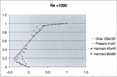
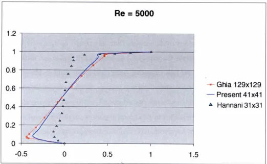
(24) Introducción, resumen y conclusiones. reducción drástica en los requerimientos de memoria, si utilizamos un almacenamiento en `skyline'.. Almacenamiento de la matriz de `rigidez' en `Skyline' para las formulaciones mixta, penalizada y segregada.. Para las formulaciones mixta y penalizada será en cambio necesario recuirir a un almacenamiento en matriz dispersa, que como sabemos es incompatible con una resolución directa del sistema. El almacenamiento en matriz dispersa se llevará a cabo mediante una técnica de `filas numeradas', y el volumen de almacenamiento será sólo el doble de los datos no nulos presentes en la matriz de rigidez. Este tipo de almacenamiento es incompatible con una resolución directa y habrá que recumir a un procedimiento de tipo iterativo. El método utilizado ha sido de tipo PBCG o método `Precondicionado de Gradientes Biconjugados', que permite obtener muy buenas aproximaciones en un número reducido de iteraciones. Los algoritmos anteriormente reseñados han sido empleados en la resolución de varios casos particulares. Los problemas académicos nos han servido para validar el algoritmo, tras lo cual el programa ha sido empleado en la resolución de varios casos prácticos. Como primer ejemplo académico, en el capítulo 3 se han utilizado los algoritmos mixto, segregado, y penalizado, para resolver el flujo en una cavidad cuadrada con velocidad tangente y unitaria en el lado superior, y condición de no deslizamiento en el resto. Este es uno de los tests más comúnmente utilizados en la verificación de las formulaciones de Navier-Stokes. Este ejemplo académico presenta varias zonas de recirculación y singularidades del campo de presiones en las esquinas superiores, lo que junto con la amplia literatura disponible al respecto, lo convierten en un problema de referencia. Los resultados obtenidos para las tres formulaciones tanteadas han sido totalmente análogos, como podía esperarse de la idéntica forma de tratar los tres tipos de formulación implementados. También se ha observado, que las. Io.
(25) Introducción, resumen y conclusiones. gráFcas de las velocidades horizontales a lo largo de una línea vertical centrada de la cavidad, están en consonancia con los resultados de referencia de [Ghia 82], [Kondo 91) y[Hannani 95], con los que se han comparado. De hecho, se han obtenido resultados muy aproximados a la solución numérica de Ghía para una malla de 129x 129 nodos (que es la solución de referencia por excelencia de los problemas de Flujo en una Cavidad), para un refinamiento de malla de tan sólo 40x40 elementos básicos de tipo Q1P0, mejorando así los resultados de Hannani y Kondo para una malla de similar refinamiento, gracias a la utilización del método de estabilización especificado en el apartado 2.6. Si bien los resultados obtenidos para los tres tipos de formulación son totalmente análogos, los tiempos de computación empleados en los mismos difieren de una manera ostentosa. Tanto en la formulación mixta como en la penalizada, se ha utilizado una resolución. del. sistema. algebraico. de tipo PBCG (Gradientes Biconjugados. Precondicionados), que consigue la convergencia de la solución para tiempos de computación más reducidos que los que se han obtenido cono resultado de emplear una formulación de tipo segregada en combinación con una resolución directa del sistema de ecuaciones. Por tanto, la economía computacional que ha supuesto la reducción en el volumen de almacenamiento de la matriz de coeficientes del sistema a resolver en el método segregado, ha sido rebasada por los mayores costes computacionales que implica la resolución de un sistema, de menor dimensión, pero de forma directa. Por otro lado, la resolución iterativa de los algoritmos mixto y penalizado, ha dado lugar a tiempos de computación similares, siendo superiores los del algoritmo penalizado en los resultados del problema del Flujo en una Cavidad. Sin embargo, en el método de penalización, la selección del parámetro e para cada problema particular, da lugar a importantes variaciones en el tiempo de computación, que puede llegar a ser menor que el empleado en una resolución mixta, si se evalúa convenientemente la magnitud del parámetro de penalización. A la vista de los resultados obtenidos para el flujo tangencial en una cavidad cuadrada, en lo sucesivo se ha utilizado indistintamente el algoritmo mixto y penalizado para la resolución de los problemas planteados. Una vez verificado el conrecto funcionamiento de las tres formulaciones de Navier-Stokes, en el capítulo 4 se presentan los resultados obtenidos con el programa en la resolución del flujo en un canal con un ensanchamiento brusco en la sección,. 11.
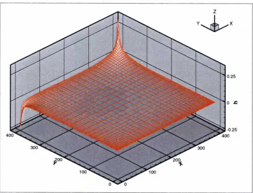
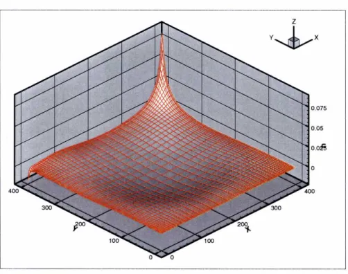
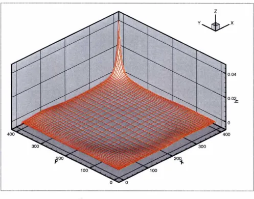
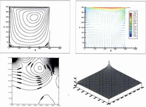
(26) Introducción, resumen y conclusiones. conocido en la bibliografía anglosajona como `Backward Facing Step'. Este es uno de. •. los problemas académicos más comúnmente utilizados en la literatura al respecto, en el que se puede observar la formación de varios vórtices de recirculación a lo largo de la longitud del canal, como consecuencia de dicho ensanchamiento en la sección. Además de numerosos resultados numéricos presentados por varios autores clásicos, existen datos experimentales de [Aimaly 83], que permiten hacer una comparación entre los datos numéricos y los reales. Esta comparación con los datos experimentales de Armaly, se hace en términos de las longitudes de reacoplamiento, que están tabuladas para distintos números de Reynolds. Los resultados obtenidos mediante la utilización del algoritmo recogido en esta tesis doctoral, mejoran apreciablemente los datos numéricos de Armaly obtenidos mediante una formulación en volúmenes finitos, acercándose de una manera manifiesta a los datos experimentales obtenidos por el propio autor. Asimismo, los resultados numéricos presentados en este trabajo están en absoluta consonancia con los conocidos resultados de [Kim 88] y[Choi 94], obtenidos a partir de formulaciones mixta y segregada respectivamente. En el capítulo 5 se evalúa el flujo en una cavidad rectangular, en la que se distribuye el caudal de entrada en tres diferentes canales de salida. Se trata ésta de una estructura que se puede encontrar con frecuencia en las plantas de tratamiento de aguas residuales. Como un primer paso, se obtienen los campos de velocidades para distintos números de Reynolds, y se observa la evolución en las líneas de corriente para los distintos casos. La observación del recorrido del fluido puede ser esencial a la hora de evaluar el dimensionamiento de una cavidad de distribución de agua, impidiendo la aparición de remolinos en caso de que las pérdidas de energía no nos interesen, o por el contrario favoreciendo la formación de los mismos, en el caso de que los fenómenos de recirculación sean favorables, para por ejemplo aumentar el tiempo de retención del fluido y favorecer así la sedimentación de partículas. También se ha introducido un término de pérdidas por fricción de tipo Manning para la resolución del flujo en esta cavidad de distribución. La inclusión de un término de Manning, análogo al definido en el apartado 1.6, permite evaluar las pérdidas por fricción de una manera empírica y como puede verse en las figuras mostradas en el capítulo 5, con resultados similares a los producidos al aumentar la viscosidad cinemática del fluido.. iz. •.
(27) Introducción, resumen y conclusiones. Aunque la solución del flujo en la cavidad de distribución se obtiene por aplicación del algoritmo permanente en solo paso, se ha resuelto también mediante incrementos progresivos de tiempo en el algoritmo no permanente. El resultado obtenido mediante la consideración de la variación del flujo a intervalos de tiempo finitos, permite observar la evolución del caudal de entrada en la cavidad hasta llegar a las condiciones de régimen, que se alcanzan en el momento en el que la última partícula que accede por el canal de entrada llega hasta el canal de salida. Como puede verse en los resultados del capítulo 5, estas condiciones de régimen se consiguen para el tiempo que la última partícula tarda en recorrer la cavidad de distribución. En el capítulo 6 se han utilizado los algoritmos de Navier-Stokes en dos dimensiones y de Aguas Someras, para resolver el flujo en un canal que se expande al doble de su anchura de forma brusca. Como era de esperar, la resolución por medio de la formulación en dos dimensiones de Navier-Stokes no asegura el cumplimiento de la ley de continuidad de la masa, y el producto de la velocidad por el área de la sección transversal no se conserva cuando se impone una ley hidrostática de presiones aguas abajo. Sin embargo, la utilización de las ecuaciones integradas en altura, permite la conservación del caudal a lo largo de todo el canal, gracias al uso del algoritmo detallado en la sección 2.5, y desarrollado por el propio autor. Finalmente, en el capítulo 7 se presentan algunos ejemplos de resolución del flujo en estructuras empleadas en la depuración de aguas residuales, a saber; decantadores de flujo horizontal, en sus variantes rectangular y circular, decantador de lamelas `LUPA' ( prototipo que está siendo desarrollado en la Escuela Técnica Superior de Ingenieros de Caminos, Canales y Puertos de La Coruña), y floculador en laberinto. La obtención de las características del flujo en todos ellos, es muy importante a la hora del dimensionamiento de estas estructuras. A modo de conclusión, este proyecto de tesis doctoral realiza un análisis exhaustivo de las ecuaciones que gobiernan el flujo incompresible y de su solución por el Método de los Elementos Finitos. Como consecuencia de ese análisis, se ha elaborado un programa que obtiene resultados óptimos en el cálculo del flujo incompresible. El programa soluciona las ecuaciones laminares de Navier-Stokes por los tres algoritmos más comúnmente utilizados dentro del marco de los elementos finitos, lo cual supone un estudio comparativo inédito. Como consecuencia, no sólo se comprueba. 13.
(28) introducción, resumen y conclusiones. que como era de esperar la solución es la misma para las tres formulaciones consideradas, sino que además la solución obtenida mejora la de varios autores de referencia, cuyos resultados se aportan para realizar la comparación, gracias a la utilización de los mecanismos estabilizadores reseñados en el texto. Además, este trabajo presenta un algoritmo, que desarrollado por el autor, permite la resolución de las ecuaciones de aguas someras gracias a la incorporación de un módulo basado en un esquema en diferencias finitas dentro del marco del Método de los Elementos Finitos. Este módulo contiene además un modelo de evaluación de los efectos turbulentos en función de la fórmula de Manning, que permite resolver la turbulencia en un gran número de los flujos relacionados con la ingeniería civil, sin perder la estructura de la ecuación de Navier-Stokes, que queda preparada para la incorporación de un modelo de turbulencia de tipo k-E,, desarrollado en el propio grupo de investigación [Bonillo 00]. Este módulo que será incorporado como un futuro desarrollo, permitirá superar con creces los modelos que, como el RMAZ de la Universidad de Brigham, se utilizan en la actualidad para el cálculo hidrodinámico de manera comercial y que hacen uso de una viscosidad turbulenta constante.. Por último, los algoritmos desarrollados han sido utilizados en la resolución de algunos casos prácticos relacionados con las estructuras de las plantas de tratamiento de aguas residuales, lo cual tiene una aplicación directa en la mejora del rendimiento de las mismas.. ia. •.
(29) CHAPTER 1. INTRODUCTION AND GOVERNING EQUATIONS. The philosophy is written in this vast book which is permanently in front of our eyes (I am referring to the universe), which nevertheless, cannot be understood if one has not learnt to understand its language and to know the alphabet in which it is written. And is written in the language of mathematics, being its script that of the triangles, circles and other geometric figures, without which we could only wander through dark mazes. Galileo Galilei,1564-1642 !I Saggiatore, VI, 232. •.
(30) Chapter 1. Introduction and governing equations. CHAPTER 1. INTRODUCTION AND GOVERNING EQUATIONS 1.1. The physical problem The aim of this thesis, framed within the numerical and hydraulic research being carried out in the Civil Engineering School of La Coruña, has been to explore the feasible numerical techniques that solve the open channel flow problems. Several formulations have been developed, implemented and validated with some available experimental and numerical data. An efficient code has been released in order to give solution to these flow problems in a stable and efficient way with great success. Once this code has been evaluated, it has been used in the resolution of some practical engineering problems related to the wastewater industry. The obtaining of the flow variables in these real cases may provide a powerful tool in order to allow for an improvement in the geometric features of the flow basins. Only through the comprehensive knowledge of the hydrodynamic variables, will the flow be not only evaluated but also fully understood. As a consequence, an adequate design of the basins and channels may be carried out, based upon an efficient and reliable numerical technique, resulting in great cost savings. The equations that rule the physical problem of the unsteady incompressible flow are based upon the Newton second law (as in any other dynamic problem), and the continuity equation, that ensures the conservation of mass in a material that has not a fixed shape. Both equalities constitute the so-called Navier-Stokes equations to be used within this work. All the flows found in civil engineering practice can be featured by the Reynolds number (UL/v, where U and L are the characteristic velocity and length of the flow and v is the kinematic viscosity that depends on the fluid nature). For small Reynolds numbers, the flow can be regarded as lan ^nar, and the streamlines are parallel to each other. As the Reynolds number is increased, a chaotic, random and intrinsically unsteady type of motion appears. ff these turbulent effects are to be solved by using the Navier-Stokes equations, a very refined mesh would be required to capture the eddies taking place on a wide range of length scales, and a special attention should be devoted. is.
(31) Chapter 1. Introduction and governing equations. to the unsteady resolution of the turbulent phenomena, that take place at a very high frequency [Versteeg 95]. The mesh refinement and the time step required for this purpose are not yet computationally affordable and a turbulence model should be implemented in order to evaluate these turbulent eddies. Most of these turbulence models are based upon decomposing the involved variables into a mean value (within a time increment) and a fluctuating term that depends on time. As a consequence of this approach, a term that evaluates the turbulent losses as a function of a so-called eddy viscosity v^, is obtained. To evaluate this eddy or turbulent viscosity, a specific turbulence model such as the k-^ model should be introduced. Making use of these turbulence models, the turbulent viscosity is calculated for each time step and position, allowing for the capturing of these eddies [Rodi 93]. Some other flow models evaluate this eddy viscosity as a constant within the flow domain, such as the RMA2 flow model developed by the Brigham University, which is one of the most commonly used programs to evaluate the flow in channels. Another approach to the turbulent problems would be to use the Manning formula. The integration in depth of the 3D Navier-Stokes equations allows for the empirical evaluation of the energy losses taking place in flows that can be regarded as shallow. The Manning formula evaluates empirically the overall energy losses taking place in the fluid flow, including those related with the turbulent effects. This formulation does not capture the turbulent eddies taking place within the fluid flow but takes into account the turbulent energy losses. Many numerical resolutions of the incompressible flow use the Manning approach to evaluate these turbulent effects. However, most of the available numerical models neglect the viscous effects compared to the turbulent ones and the viscous term is dropped from the equations. Some other Navier-Stokes flow models ignore the turbulent effects, and make use of the plain Navier-Stokes equations. As a consequence, they can only be used for a moderate Reynolds number, even when a stabilization technique is used, and even for very refined meshes. In comparison to those which evaluate the turbulence on a Manning basis, these models provide a finer approach to the problems characterised by a moderate Reynolds number, as they keep the real forces balance.. 16. •.
(32) Chapter 1. Introduction and governing equations. The formulation presented in this work solves the Navier-Stokes equations making use of a SUPG type stabilization technique, allowing for the resolution of the flow when the Reynolds number is of a moderate order. A Shallow Water algorithm that incorporates a Manning ternn is also presented, nonetheless this formulation does not get rid of the viscous term, allowing for the incorporation of a turbulent model that evaluates the eddy viscosity as a function of time and space. A k-E turbulence model has been developed in our research group and it will be added as a further development. This module has been proved to work properly when used in connection with the RMA2 model, which uses a constant eddy viscosiry. Once the code has been validated, it will be used to evaluate the flow in some water treatment engineering problems, and their results will be presented. Some of these wastewater flow problems will be used as part of the research being carried out in the sanitary engineering area of the Escuela Técnica Superior de Ingenieros de Caminos, Canales y Puertos de La Coruña.. 1.2. Numerical resolution of the flow problem. The Navier-Stokes equations have an analytical solution for a very small set of simple flows. In any other case a numerical procedure giving an approximate solution of the flow, should be used in its resolution. Many numerical techniques have been developed for the resolution of the incompressible flow. The four main groups into which these numerical techniques can be separated, are the Finite Difference, Finite Volume, Spectral and Finite Element Methods. The Finite Difference Method is based upon the use of the finite difference approximation of the derivatives included in the equations to be solved, being used by many authors in the resolution of some particular incompressible flow problems [Richtmyer 67], [Roaches 76], [Baker 83], [Katopodes 84], [Smith 85]. The Spectral Method approximates the unknowns in the Navier-Stokes equation by the use of the Fourier series or the Chebyshev polynomials [Gottlieb 77], nonetheless the Spectral Method shows some important problems when the boundary conditions are not periodic [Canuto 88]. The Finite Volume Method was first developed as a special finite. i^.
(33) Chapter 1. Introducrion and governing equations. difference formulation to be used in fluids, based upon the splitting of the domain into a finite number of control volumes. The governing equations are integrated over all the control volumes of the domain, and the discretization to be carried out involves the use of some finite difference type approximations. There are many different versions of the Finite Volume Method that have been extensively used in the resolution of the NavierStokes equations [Patankar 80], [Roe 89], [Hubbard 93], and still are used with very good results. These difference based algorithms can be regarded in a unified way, as specific criteria within the weighted residuals framework, upon which the Finite Element Method is based [Finlayson 72]. The Finite Element Method will be the one used in this doctoral thesis, and will be further considered in the next chapter and throughout the text. Apart from those, there are some other numerical methods, that such as the Meshless [Oñate 95, 96] or the Boundary Element Methods [Onishi 84], [Brebbia 86], have been recently used to solve the Navier-Stokes equations with very promising results. 1.3. Finite element resolution of the flow problem. The Finite Element Method is a numerical procedure for solving the differential equations that govern a wide variety of physical problems. This technique subdivides the domain of definition into a finite number of smaller regions, and uses the weighted residuals method so as to transform the governing differential equations into a set of discrete integral equations. This system of equations gives as a result, the value of the unknowns in the nodal points of the basic elements, being an approximation to the problem posed in the governing equations. The Finite Element Method was first developed in the fifties by Turner and Clough so as to solve some structural problems of the aeronautical industry [Turner 56]. The good results obtained for structural analysis were soon transported to other physical problems, such as elementary flow and electromagnetism problems [Zienkiewicz 65]. The appearance of `The Finite Element Method' in 1967 by Zienkiewicz and Taylor [Zienkiewicz 1989], establishes the basis of this numerical technique. Since then, and thanks to an amazing improvement in the computer performances in the second half of this century, the Finite Element Method is the. ^s. •.
(34) Chapter 1. Introdnction and governing equations. numerical technique most commonly used in the approximate resolution of a wide variety of the physical problems arisen within these years. The application of the Finite Element Method to the flow problems requires some modifications with respect to the formulation used for the structural stress analysis problems, that were its first application. Some of these modifications have been borrowed from the finite difference or finite volume approaches, and many others have been specifically developed for finite elements. In the early seventies we find many works regarding not only the mere existence and consistency of these flow problems [Ladyzhenskaya 69], [Babuska 71], [Brezzi 74], but also many works that give a finite element solution to the Navier-Stokes equations [Baker 71 ], [Oden 72], [Fortin 72], [Crouzeix 73], [Jamet 73], [Taylor 73], [Shen 76], [Zienkiewicz 76]. Since then, the Finite Element Method is a powerful tool for the resolution of the Navier Stokes equations, which will be used in this doctoral thesis so as to solve the incompressible flow, as may be seen in the sections to follow. The material we are going to deal with, when solving the flow, is of a fluid nature, and therefore it has not a fixed shape, which is instead a function of time. In addition to Newton's second law, that rules any dynamic problem, an equation that ensures for the conservation of mass should be verified. Moreover, the Navier-Stokes equations are a set of differential equations with respect to both space and time in which both the pressure and the velocity are the unknowns. As a consequence, the finite element formulation used for the conventional structural analysis cannot be applied straightforwardly. When applying the finite element analysis to the problems of the rigid body, the weighted residual method can be exclusively applied to the Newton second law, which for statics clearly turns out to be the equilibrium equation; there is no use in imposing the conservation of mass to a set of materials which do not lose their shape. On the contrary, when dealing with fluids, the shape is not any more conserved, and apart from stating the equilibrium of momentum, we have to ensure for the continuity of mass. Consequently, we have two equations to be verified at the same time, and the finite element formulation should also account for the verification of both. The only set of unknowns in the conventional structural analysis is that of the displacements, as a. 19.
(35) Chapter 1. Introduction and goveming e^uations. consequence, the system obtained thanks to the application of the Finite Element. t. Method, gives the displacements in the structure depending on the stiffness matrix (that features the structure), and the load vector. In the flow problems, we are headed towards the so-called mixed Finite Element Methods, in which both the velocity and pressure set of unknowns have to be treated simultaneously. Depending on how these two sets of equations and unknowns are tackled, several different approaches are developed. The most intuitive of these approaches would be simply to carry out a similar analysis for the continuity equation to that used for the momentum equation, carrying along both velocity and pressure as the unknowns up to the end of the problem, [Baker 71] [Oden 72], [Zienkiewicz 76]. This apparently straightforward way of dealing with our equations is not as simple as it appears to be, and it may be the reason of the obtaining of a meaningless solution when used in connection with a faulty basic element [Babuska 71], [Taylor 73], [Brezzi 74]. Besides a big expense in the storing memory, the so-called mixed formulation, leads to some consistency problems in the obtaining of the solution when a wrong choice in the basic functions has been made. As a consequence, many different formulations have been used trying to overcome these difficulties. In this work, some of these different approaches will be employed and discussed. The 2D Navier-Stokes equations assume a flow that takes place on a twodimensional plane, and it is therefore laminar in that sense. The Shallow Water formulation has been also considered as a way of including the third dimension in the calculations, being able to give a meaningful solution for flows in which the depth is small compared to the horizontal dimension. The integration in depth of the 3D NavierStokes formulation, causes the dependence of the continuity equation with respect to depth, and consequently the appearance of some quasi-non-linear terms that depend on both the velocity and the depth. These equations are solved thanks to a newly developed iterative algorithm, which will be solved on a mixed formulation basis to be regarded in full in section 2.5. The use of a Galerkin formulation, that takes weighting functions equal to trial functions, when solving the Navier-Stokes equations, may lead to some problems of instability in the flow solution by the Finite Element Method. To avoid this difficulty,. Zo. !.
(36) Chapter 1. Introduc^on and goveming equations. some so-called stabilization procedures have been released since the MAFELAP conference in 1975 [Zienkiewicz 76]. The stiffness matrix resulting from structural problems solved by the Finite Element Method is symmetric, instead the `stiffness' matrix obtained for fluids is non-symmetric and the use of symmetric weighting functions may lead to some instability problems. The faster the flow turns, the more non-symmetric the coefficient matrix becomes. In practice this is featured by the appearance of some spurious node-to-node oscillations also known as `wiggles' . One way of avoiding these oscillations is to carry out a refinement in the mesh, such that convection no longer dominates on an element level, but this refinement turns to be a memory resources sink. This point will be avoided in this work by the use of an stabilization technique of the SUPG type, for all the algorithms considered in it. The SUPG (Streamline/Upwinding Petrov-Galerkin) technique, first developed by Brookes [Brookes 82], succeeds in eliminating the spurious velocity field, without carrying out a severe refinement in the mesh, by considering weighting functions that differ from trial functions in an upwinding term. Tfiis method was first released for the transport equation, and its generalisation to the Navier-Stokes equation brings an additional problem; that is the appearance of an excessive diffusion normal to the flow. The SUPG method eliminates this spurious crosswind diffusion by considering an `artificial' diffusion that acts only in the direction of the flow. These aspects will be further considered in section 2.6. All the particulars regarded in this introduction and some others, will be further discussed in the following chapters. A code will be written based upon these particulars, and will be also validated by its comparison with available numerical and empirical reference results. Once the program has been validated, it will be used in the resolution of some wastewater problems. In the present chapter, the equations that rule the viscous incompressible flow will be derived and presented, together with all the assumptions carried out in their securing. Once the 2D Navier-Stokes and the Shallow Water equations have been presented, chapter two will be devoted to the finite element resolution of these equations by several different algorithms of the mixed, penalry and segregated type. Chapter two will also focus on the definition of an stabilising technique of the SUPG type, in order to avoid the instability showing up in the solution. u.
(37) Chapter 1. Introduction and goveming e^uations. beyond a certain Reynolds number, and also in the treatment to be given to the viscous effects. An especial mention to the solver used in the resolution of the resulting system of differential, non-linear equations will be carried out at the end of chapter two. In chapter number three, the mixed, penalty and segregated 2D formulations are validated by comparing the results obtained thus, with referehce results by other authors on the Cavity Flow benchmark problem. As a result, it is shown how these algorithms prove to yield a better accuracy for a less refined mesh, compared to the one obtained by other authors and regardless of the algorithm employed in the calculations, that only plays an important role in the computational efficiency yielded. In chapter number four a comparison is made among the experimental results obtained for the Backward Facing Step benchmark problem of Armaly et al. [Armaly 83) and the results obtained by using the 2D algorithm proposed in this doctoral thesis. As a result, the solution obtained by the present author seems to be in a better agreement with the experimental results than those obtained numerically by Armaly as can be regarded in the information provided in this chapter. Chapter number five is devoted to the analysis of the influence of the consideration of the Manning term in the formulation. The Manning term as explained in chapter two manages to evaluate the turbulent effects that show up , in the real flows when a certain Reynolds number is overcome. Beyond that number, the turbulence can not be denied in order to give solution to the physical phenomenon, and the consideration of the Manning coefficient manages to evaluate the overall turbulent energy losses, as shown in the examples provided in this chapter, that also considers the evolution in time of the unsteady algorithm. Chapter six is concerned with the comparison between the 2D laminar and Shallow Water formulations. As it was expected, the 2D algorithm dces not manage to evaluate the conservation of mass in a three-dimensional manner, especially when the conditions of the flow force a change in the depth of the flow. Nonetheless the Shallow Water algorithm presented in chapter two provides an optimum tool for this purpose. Finally, chapter seven is devoted to the resolution of some real flow problems related with the wastewater industry, and provides some results very valuable in the designing of the water treatment plants.. ^z. •.
(38) Chapter 1. Introduction and goveming equations. 1.4. Governing equations Our first task will be to obtain the governing equations that rule our physical problem; this is the resolution of the unsteady, incompressible flow. As in any other dynamic problem, the equation we are going to refer to, is the Newton second law, which gives the variation in the momentum as the summation of the acting forces on the volume of integration. To this condition we should add another one, due to the fact that we are dealing with a shape-changing matter in which we have to ensure the continuity of mass. Both equations make up the Navier-Stokes equations. These equations are named after their discoverer, the French civil engineer Claude-Louis Navier (1785-1836), who in 1821 formulated the equations that rule the incompressible flow. The Navier-Stokes equations also bear the name of the Irish mathematician George Gabriel Stokes (1819-1903), who not knowing the previous discoveries made by Navier, Poisson and Saint-Venant, re-obtained the Navier-Stokes equations for slightly different assumptions, and published these works in 1845. The Irish mathematician gives also his name to the simplified version of the Navier-Stokes equations, in which the convective terms are dropped. The complexity of the Navier-Stokes equations leads to the use of some other simplified governing equations. Most of the difficulties found in the resolution of the Navier-Stokes equations are derived from the presence of the convective term in the dynamic equations, as will be explained later. The Stokes equations assumes ^that the convective part of the dynamic equation in the Navier-Stokes formulation is not. •. significant and can be denied [Carey 84]. This assumption removes the non-linearities from the Navier-Stokes equations, and consequently avoids most of the problems that the consideration of this term causes in the resolution of the flow when a large enough Reynolds number features the flow. In fact, the convective acceleration usually dominates the flow, and the Stokes assumption can only be considered for the so-called `creeping flows,' or in other words, slow flows with scant depth. Therefore, a convective-term-including formulation is required in order to solve the real flow problems, and the Stokes simplification will not be used in this work, apart from comparison purposes.. 23.
(39) Chapter 1. Introductio^n and goveming equations. The 2D Navier-Stokes equations will be used in this thesis to solve many benchmark problems of the related literature with very good results, as will became clear later in the text. The 2D or laminar (in the sense of planar) Navier-Stokes equations do not take into account the third dimension in space, ^and provide with the velocities and pressures of a theoretical planar flow. Nevertheless, for many real flow problems, the third dimension in space is very important and the 3D Navier-Stokes equations should be considered. The three-dimensional Navier-Stokes equations result in a very large-dimensioned system of equations, that involves very high computational costs. Moreover the 3D schemes present a great difficulty in the treatment of the free surface. For flows in which the horizontal dimension is small compared to depth, the Shallow Water formulation can be employed as a simplification of the 3D NavierStokes equations, [Weiyan 92]. The Shallow Water equations are a simplification of the Navier-Stokes equations, which can be used when the main direction of the flow is the horizontal one and the distribution of the horizontal velocity along the vertical direction can be assumed as uniform. These equations assume that the vertical acceleration of the fluid is negligible and that a hydrostatic distribution of the pressure can be adopted. The Shallow Water equations are obtained by integrating the 3D Navier-Stokes equations in depth, and give a meaningful solution for flows in which the horizontal dimension is small compared with the depth. When a 2D Navier-Stokes equation is used, no attention is paid to the third dimension in space, and the results are based upon a 2D approach to the flow problem. Therefore, the continuity equation is only held on a 2D basis. So as to get some information about the variations in depth along the flow, either a 3D Navier-Stokes equation or the Shallow Water equations (if the flow can be regárded as shallow), should be used. The Shallow Water equations are solved in this work for that purpose. Before obtaining the Navier-Stokes equations, let us first define the system of reference we are going to use to translate our physical problem into mathematical language. Due to the variation in shape of fluids, the traditional Lagrangian reference system used in the mechanics of the rigid bodies is no longer useful. When using Lagrangian co-ordinates in fluids, we are going to express all the quantities with respect. ^. •.
Figure
+7
Documento similar
The Blow Up Issue for Navier-Stokes Equations If the solution of the Euler equations with initial data u (0) is smooth on a time interval [0, T ] then the solutions of the
In two dimensions, we have considered the prob- lem of prescribing Gaussian and geodesic curvatures on topological disks via confor- mal transformation of the metric, while we
On the other hand, in terms of control in wind farms, the authors of [5] mention vari- ous wind measurement methods which allow measurements to be made before and after the creation
The numerical re- sults presented in this chapter serve to demonstrate the feasibility of the nite element formulation proposed to approximate the three- eld Navier-Stokes
For the methods analyzed in Sections 3 – 5, error estimates with constants independent of inverse powers of the diffusion parameter are derived with the help of stabilization terms
An initial numerical study of the transducer was done using the finite element method (FEM) software COMSOL Multiphysics®. The aim of this design was to obtain a very resonant system,
In this paper we analyze a finite element method applied to a continuous downscaling data assimilation algorithm for the numerical approximation of the two and three dimensional
The results obtained using the new technique are validated by comparing them with those obtained using a finite-element technique, and with a standard IE implementation using
