Development, calibration and validation of a dynamic genome scale metabolic model of saccharomyces cerevisiae

Texto completo

(1)PONTIFICIA UNIVERSIDAD CATOLICA DE CHILE ESCUELA DE INGENIERIA. DEVELOPMENT, CALIBRATION AND VALIDATION OF A DYNAMIC GENOME-SCALE METABOLIC MODEL OF SACCHAROMYCES CEREVISIAE. BENJAMÍN J. SÁNCHEZ. Thesis submitted to the Office of Research and Graduate Studies in partial fulfillment of the requirements for the Degree of Master of Science in Engineering Advisors: EDUARDO E. AGOSIN J. RICARDO PÉREZ-CORREA Santiago de Chile, January, 2014  2014, Benjamín J. Sánchez.

(2) PONTIFICIA UNIVERSIDAD CATOLICA DE CHILE ESCUELA DE INGENIERIA. DEVELOPMENT, CALIBRATION AND VALIDATION OF A DYNAMIC GENOMESCALE METABOLIC MODEL OF SACCHAROMYCES CEREVISIAE. BENJAMÍN J. SÁNCHEZ. Members of the Committee: EDUARDO E. AGOSIN J. RICARDO PÉREZ-CORREA JORGE R. VERA ALEJANDRO MAASS PABLO PASTÉN. Thesis submitted to the Office of Research and Graduate Studies in partial fulfillment of the requirements for the Degree of Master of Science in Engineering Santiago de Chile, January, 2014.

(3) “I don't know anything, but I do know that everything is interesting if you go into it deeply enough”. Richard P. Feynman. ii.

(4) ACKNOLEDGMENTS I am deeply thankful of many people that have helped me through my thesis. First I would like to thank both of my advisors, Professor Eduardo Agosin and Professor Ricardo Pérez-Correa, for accepting me as their student, trusting me and encouraging me to always push forward in my investigation. Also, thanks to the members of the committee that evaluated this work and provided me with valuable feedback to further enrich the manuscript.. I would also like to thank all the members from the biotechnology laboratory, in which I did all of my experiments; many thanks to Waldo Acevedo, Martín Cárcamo, Mariana Cepeda, Martín Concha, Jonathan Leon, Trinidad Pizarro, Pedro Saa, Fernando Silva, Jorge Torres, Paulina Torres and Felipe Varea for their valuable assistance, and to Marianna Delgado, Javiera López, Alejandra Lobos and Isabel Moenne for making me feel as part of a family. Thanks also to Professor Claudio Gelmi for his wise recommendations and suggestions.. Special thanks to my parents, who always have supported me in my decisions, even though sometimes they did not agreed entirely. Thanks also to my 6 siblings and my nephew, for always making my smile, and to my girlfriend Macarena, for believing in me specially when occasionally I did not. Special acknowledgments to my friends and family that read my manuscript and helped making it accessible to a broader audience.. Finally, I would like to thank the Chilean governmental agency CONICYT, for partly financing this project (grant Fondecyt #1130822) and also my graduate studies (grant CONICYT-PCHA/Magíster Nacional/2013 – #221320015).. iii.

(5) GENERAL INDEX Page Table Index…………………………………………………………………………...vii Figure Index ...................................................................................................... ……...x Abstract……………………………………………………………………………...xiv Resumen …………………………………………………………………………….xv 1. Introduction......................................................................................................... 1 1.1 Flux Balance Analysis................................................................................ 1 1.2 Dynamic FBA ............................................................................................ 2 1.3 Parameters in dFBA ................................................................................... 3 1.4 Hypothesis and Objectives ......................................................................... 5 1.5 Organization of the Document ................................................................... 7. 2. Modeling ............................................................................................................. 8 2.1 Model Formulation..................................................................................... 8 2.2 Metabolic Block ....................................................................................... 10 2.3 Dynamic Block......................................................................................... 12 2.4 Kinetic Block ........................................................................................... 14 2.4.1 Glucose Consumption .................................................................... 14 2.4.2 Oxygen Consumption .................................................................... 15 2.4.3 Secondary Metabolite Production.................................................. 15 2.4.4 ATP Maintenance .......................................................................... 16 2.4.5 Biomass Requirements .................................................................. 16 2.4.6 Gene Expression ............................................................................ 17 2.5 Parameter Estimation ............................................................................... 19. 3. Materials and Methods ..................................................................................... 22 iv.

(6) 3.1 Strains and Conditions Assessed .............................................................. 22 3.2 Experimental Setup .................................................................................. 23 3.3 Assay Methods ......................................................................................... 28 3.4 Reparameterization Analysis ................................................................... 29 3.4.1 General Methodology of Procedure ............................................... 29 3.4.2 Pre/Post Regression Diagnostics ................................................... 31 3.4.3 Cross-Calibration ........................................................................... 33 4. Results and Analysis ......................................................................................... 34 4.1 Pre/post Regression Results ..................................................................... 34 4.1.1 Identifiability Analysis .................................................................. 34 4.1.2 Sensitivity Analysis ....................................................................... 36 4.1.3 Significance Analysis .................................................................... 37 4.2 Reparameterization Results ...................................................................... 37 4.2.1 Parameter Solutions ....................................................................... 37 4.2.2 Fittings ........................................................................................... 41 4.3 Cross-Calibration Results......................................................................... 46 4.3.1 Best Solutions ................................................................................ 47 4.3.2 Nutrient Limitation Importance ..................................................... 49 4.3.3 Strain Performance ........................................................................ 49 4.4 Approach Limitations............................................................................... 50 4.4.1 Parameters not Included in the Study ............................................ 50 4.4.2 Fed-batch Parameters ..................................................................... 51 4.4.3 Gene Expression Parameters ......................................................... 52 4.4.4 Additional Considerations ............................................................. 53. 5. Conclusion ........................................................................................................ 55. 6. Abbreviations .................................................................................................... 57. 7. Outreach ............................................................................................................ 59 v.

(7) References .................................................................................................................. 60 Appendix .................................................................................................................... 68 Appendix A: Supplementary Tables .......................................................................... 69 Appendix B: Supplementary Figures ......................................................................... 88. vi.

(8) TABLE INDEX. Page Table 2-1: Computational time spent for the different algorithms in the 3 different computers used, and for the 2 typical types of fermentation: anaerobic batch (AB) and aerobic fed-batch (AF).................................................................. 10. Table 2-2: Parameter estimation details. The symbols, names and units of each parameter analyzed in this study are shown. Initial values, lower and upper bounds for parameter estimation are also displayed. .................................. 20. Table 3-1: Composition of all defined-media employed in this study: batch and feed media for aerobic cultivations, and the 2 different anaerobic batch media used (20 [g/L] and 80 [g/L] of glucose, respectively). ................................. 23. Table 4-1: Percentage of times that each parametric problem arose in (A) aerobic and (B) anaerobic calibrations. Identifiability was calculated as correlations between each pair of parameters, relative sensitivity was averaged among all variables, and significance was calculated using coefficients of confidence. ...................................................................................................................... 35. Table 4-2: The fixed and estimated parameters are presented along with their CC (only for the estimated parameters), after applying the pre/post regression procedure in the (A) aerobic cultivations and (B) anaerobic cultivations. ... 40. Table 4-3: The objective function value is presented for all 16 cultivations, after the initial calibration (Initial F) and after applying the iterative procedure (Final F).. ................................................................................................................. 42. vii.

(9) Table 4-4: The results of the cross calibration are presented for (A) aerobic and (B) anaerobic cultivations. Each CCC was calculated as indicated in Equation 21. The mean CCC for each solution is also presented, and the best one for each cultivation condition (aerobic/anaerobic) is blackened .…...……...…47. Table 4-5: Averaged CCCs between duplicates for (A) aerobic and (B) anaerobic cultures.......................................................................................................... 50. Table A-1: Calibration comparison between Yeast 5 and Yeast 6 for two typical cultivations. The objective function value (F) and the computation time (t) are displayed................................................................................................ 69. Table A-2: The SGD names of the essential genes for aerobic and anaerobic growth in the genome-scale metabolic model Yeast 5 (Heavner et al., 2012) are presented. The genes that are only essential for one condition but not for the other one are highlighted. As it has been done regularly (Edwards & Palsson, 2000; Zomorrodi et al., 2012), a gene is defined essential if by deleting it (constraining in zero all associated reaction fluxes) growth is not achieved when performing FBA................................................................... 70 Table A-3: All solutions with no identifiability, sensitivity and significance problems are shown below, for (A) aerobic and (B) anaerobic cultivations. The fixed parameters are highlighted, and the chosen solution in each case is highlighted with a bold box. ......................................................................... 71. Table A-4: The correlation matrices of the reparameterized models are presented for (A) aerobic and (B) anaerobic cultivations. ........................................................ 83. viii.

(10) Table A-5: The deleted genes for the different attained thresholds are displayed for each of the (A) aerobic and (B) anaerobic cultivations. This table together with Table 4-2 shows that cases which have at least one gene deleted have the lower thresholds, as expected. The associated enzymes for each gene are: YHR096C → hexose transporter with moderate affinity for glucose. YJR048W,. YMR256C,. oxidoreductase;. YOR065W. YML054C. →. ferrocytochrome-c:oxygen. (S)-lactate:ferricytochrome-c. oxidoreductase;. YML120C. YMR009W. 2,3-diketo-5-methylthio-1-phosphopentane. →. →. →. NADH:ubiquinone. 2-. oxidoreductase; degradation. reaction; YMR145C NADH → dehydrogenase, cytosolic/mitochondrial; YOL151W → L-lactaldehyde:NADP+ 1-oxidoreductase. .......................... 87. ix.

(11) FIGURE INDEX. Page Figure 1-1: Typical fitting problems that arise when a model has too many parameters. (A) An example of a parameter that is not significantly estimated, because the confidence interval is larger than its value. (B) An example of a nonsensitive parameter, because different values yield the same result in the associated variable. (C) An example of two parameters not identifiable, because different value combinations will result in the same output. (D) An example of parameter overfitting, in which an excessive number of parameters are proposed to explain the data. ................................................ 4. Figure 2-1: General scheme to solve the dFBA model. V is volume [L], X is biomass concentration [g/L], G is extracellular limiting substrate (glucose) concentration [g/L], Pk accounts for the different extracellular product concentrations [g/L], Fin(t) is the feed function for the fed-batch cases [L/h], O2(t) is the predefined oxygen presence or absence, t is time [h] and tF is the fermentation duration [h]. ................................................................ 9. Figure 2-2: Derivation of the FBA equations using a small metabolic network. Adapted from (Becker et al., 2007). .......................................................................... 12. Figure 2-3: Dynamic system modeled. The vessel represents the bioreactor and the figure inside of it represents yeast. .............................................................. 13. x.

(12) Figure 3-1: Photograph of one of the bioreactors used. Both temperature/oxygen and pH probes are behind the motor and therefore not shown. (1) DC motor connected to the bioreactor agitator. (2) (Filtered) gas entrance to the bioreactor. (3) Condenser. (4) Off gas exit (to CO2 and O2 analyzer). (5) Sampler (behind the condenser). (6) Bioreactor (glass flask inside the glass jacket). (7) Water entrance to the glass jacket. (8) Water exit of the glass jacket. .......................................................................................................... 25 Figure 3-2: P&ID of the system used for all cultivations. Nomenclature used: AT → Analysis Transmitter. AR → Analysis Recorder. ARC → Analysis Recorder & Controller. TT → Temperature Transmitter. TRC → Temperature Recorder & Controller. FC → Flow Controller (Not used in anaerobic conditions). ................................................................................. 26. Figure 3-3: The temporal evolutions of the design growth rate (µset) and a given feed rate (F) for experimental conditions 1 (C = 0.14 [1/h]) and 2 (C = 0.07 [1/h]) are displayed, with t = 0 as the feed starting point. Condition 1 has a quicker decay in µset than condition 2, and therefore has a slower F than condition 2. For F visualization, typical experimental conditions were selected: Vi = 0.4 [L] and Xi = 4 [g/L] (for further details refer to Equation 14). ............. 27. Figure 3-4: Methodology used in this study for obtaining dFBA models with sensitive, uncorrelated and significant parameters. As an example, a solution with 5 parameters is analyzed. ............................................................................... 30. xi.

(13) Figure 4-1: The average number of iterations performed by the procedure for aerobic cultivations is displayed in a logarithmic scale, along with all possible combinations and the non-problematic solutions achieved. The total number of combinations was calculated in each case as (. 19 ), where 19 is i. the total number of parameters and i is the corresponding number of fixed parameters. .................................................................................................. 38. Figure 4-2: The average number of iterations performed by the procedure for anaerobic cultivations is displayed in a logarithmic scale, along with all possible combinations and the non-problematic solutions achieved. The total number of combinations was calculated in each case as (. 14 ), where 14 is the total i. number of parameters and i is the corresponding number of fixed parameters. .................................................................................................... 39. Figure 4-3: (previous page) Calibrations obtained with the dFBA model after applying the pre/post regression analysis to the aerobic cultivations. Each graphic displays the experimental measures for biomass (♦), glucose (■), ethanol (▲), glycerol (×), citric (+) and lactic acid (●), together with the corresponding. model. prediction. (continuous. lines),. for. different. experimental conditions: (A-B) N30 strain, slow feed. (C-D) N30 strain, fast feed. (E-F) EC1118 strain, slow feed. (G-H) EC1118 strain, fast feed. ....... 44. xii.

(14) Figure 4-4: (previous page) Calibrations obtained with the dFBA model after applying the pre/post regression analysis to the anaerobic cultivations. Each graphic displays the experimental measures for biomass (♦), glucose (■), ethanol (▲), glycerol (×), citric (+) and lactic acid (●), together with the corresponding. model. prediction. (continuous. lines),. for. different. experimental conditions: (A-B) N30 strain, small G0. (C-D) N30 strain, large G0. (E-F) EC1118 strain, small G0. (G-H) EC1118 strain, large G0. .. 46. Figure B-1: Relative sensitivity for each parameter in each state variable for the 8 aerobic cultivations. For every parameter, each bar represent the impact on one state variable; from left to right the bars are biomass, glucose, ethanol, glycerol, citric and lactic acid. .................................................................... 88. Figure B-2: Relative sensitivity for each parameter in each state variable for the 8 aerobic cultivations. For every parameter, each bar represent the impact on one state variable; from left to right the bars are biomass, glucose, ethanol, glycerol, citric and lactic acid. .................................................................... 89. xiii.

(15) ABSTRACT In the biotechnology industry it is fundamental to count on accurate mathematical models that describe a microorganism with detail, so we can make predictions and avoid performing an excessive amount of experiments. Dynamic flux balance analysis (dFBA) has been widely used to simulate batch and fed-batch cultivations, the most recurrent industrial biotechnological processes; nonetheless, only a few of these models have been calibrated and validated under different experimental conditions. Moreover, to date, the importance of the different parameters usually used in this kind of models has not been appropriately addressed. In this work, we present a genome-scale dFBA model of Saccharomyces cerevisiae calibrated for the first time using both aerobic fed-batch and anaerobic batch data, together with a novel procedure to determine which parameters of the model are relevant for calibration (in terms of sensitivity, identifiability and significance). The proposed dFBA model comprises several kinetics including suboptimal growth, glucose consumption, ATP maintenance, biomass requirements and secondary metabolite production rates, and also integrates gene expression data. On the other hand, the calibration procedure uses metaheuristic optimization and pre/post regression diagnostics, and fixes iteratively the parameters that do not have a significant role in the model, so models with a reasonable amount of parameters can be proposed. Finally, the models attained are cross-calibrated to assure predictability. Using this approach, we showed that glucose consumption, suboptimal growth and production rates are far more useful for calibrating the model than gene expression constant Boolean rules, biomass requirements or ATP maintenance. Furthermore, confident models were obtained (for the first time in dFBA modeling) with sensitive, uncorrelated and significant parameters, and that are also able to calibrate numerous experimental settings. These robust and predictive yeast dFBA models will be useful to design optimized strains for metabolic engineering applications.. Keywords: GSMM, dFBA, metaheuristic optimization, yeast, nonlinear dynamic model, parameter estimation, sensitivity analysis, metabolic engineering. xiv.

(16) RESUMEN En la industria biotecnológica es fundamental contar con modelos matemáticos precisos que describan un microorganismo en detalle, de manera de que podamos hacer predicciones sin tener que incurrir en una cantidad excesiva de experimentos. El análisis dinámico de balance de flujos (dFBA) se ocupa regularmente para simular cultivos batch y fed-batch, los procesos industriales biotecnológicos más recurrentes; sin embargo, sólo unos pocos de estos modelos han sido calibrados y validados bajo diferentes condiciones experimentales. Además, a la fecha, la importancia de los diferentes parámetros usualmente utilizados en este tipo de modelos no ha sido debidamente estudiada. En este trabajo presentamos un modelo dFBA a escala genómica de Saccharomyces cerevisiae calibrado por primera vez con datos tanto de cultivos fedbatch aeróbicos como batch anaeróbicos, junto con un nuevo procedimiento para determinar cuáles parámetros del modelo son relevantes para calibración (en términos de sensibilidad, identificabilidad y significancia). El modelo dFBA contiene varias cinéticas, incluyendo crecimiento sub-óptimo, consumo de glucosa, ATP de mantenimiento, requerimientos de biomasa y producción de metabolitos secundarios. También integra datos de expresión génica. Por otro lado, el procedimiento de calibración usa optimización metaheurística y análisis de pre/post regresión, y fija iterativamente los parámetros que no tienen un rol significativo en el modelo, de manera de obtener modelos con un número razonable de parámetros. Finalmente, a los modelos obtenidos se les hizo una calibración cruzada para asegurar que sean predictivos. Usando este enfoque, mostramos que el consumo de glucosa, el crecimiento sub-óptimo, y las tasas de producción son mucho más útiles para calibrar los modelos que reglas Booleanas constantes de expresión génica, los requerimientos de biomasa o el ATP de mantenimiento. Más aún, se obtuvieron modelos dFBA confiables (por primera vez) con parámetros sensibles, significativos y sin correlaciones, y que a la vez son capaces de calibrar varias condiciones experimentales. Estos modelos dFBA de levadura robustos y predictivos serán útiles para diseñar cepas optimizadas para diversas aplicaciones en ingeniería metabólica. xv.

(17) Palabras Claves: Modelos metabólicos a escala genómica, análisis dinámico de balance de flujos, optimización metaheurística, levadura, modelos dinámicos no lineales, estimación de parámetros, análisis de sensibilidad, ingeniería metabólica.. xvi.

(18) 1. 1. INTRODUCTION 1.1. Flux Balance Analysis. Mathematical modeling is a fundamental tool in metabolic engineering and the biotechnology industry since it overcomes the need for excessive experiments to validate a certain biological hypothesis (Kitano, 2002). Among the different modeling tools, flux balance analysis (FBA) is widely employed (Park, Kim & Lee, 2009). Using mass balances, under pseudo steady-state assumption and with an underlying objective function (Orth, Thiele & Palsson, 2010), FBA can predict the behavior of the whole cell metabolism. Since it was first validated as a predictive tool (Varma & Palsson, 1994), there have been numerous efforts for improving its predictive performance (Copeland et al., 2012).. FBA applications have increased considerably since the introduction of genome-scale metabolic models (GSMM) (Edwards & Palsson, 2000; Osterlund, Nookaew & Nielsen, 2012). A GSMM consists of a fully detailed metabolic network, including not only most metabolites and reactions of the studied organism, but also most metabolism-associated genes (Henry et al., 2010; Thiele & Palsson, 2010). Hence, predictions can be computed to assess the impact of genetic modifications in metabolism, in order to overproduce a certain compound of interest. In the case of Saccharomyces cerevisiae (budding yeast), Förster and associates proposed the first GSMM in 2003 (Förster, Famili, Fu, Palsson & Nielsen, 2003), and since then numerous other versions have been reported (Nookaew, Olivares-hernández, Bhumiratana & Nielsen, 2011). Particularly, in 2008 a consensus model was developed in a world-wide jamboree of the yeast metabolic engineering community (Herrgård et al., 2008). This model was further expanded to improve biochemical coverage, connectivity and knockout predictability (Dobson et al., 2010; Heavner, Smallbone, Barker, Mendes & Walker, 2012; Heavner, Smallbone, Price & Walker, 2013)..

(19) 2. Although all the aforementioned efforts have contributed to gain knowledge of yeast’s steady-state metabolism and to make accurate predictions for the overexpression of high-value metabolites in mutant strains (Oberhardt, Palsson & Papin, 2009), the kinetics and physiology of yeast can be better understood in a dynamic setting, with changing environmental conditions and variable cell-density, which are standard conditions of industrial processes (Gianchandani, Chavali & Papin, 2010; Oddone, Mills & Block, 2009).. 1.2. Dynamic FBA. Dynamic FBA (dFBA) is an extension of FBA in which, under the pseudo-steady state premise for short time steps (Stephanopoulos, Aristidou & Nielsen, 1998), the variations of the extracellular metabolite concentrations modify the FBA problem restraints (using uptake and/or production kinetics), and in return the FBA solution modifies the consumption/secretion rates for the bioreactor’s dynamic equations (Mahadevan, Edwards & Doyle III, 2002; Sainz, Pizarro, Pérez-Correa & Agosin, 2003). This approach offers the main advantage of combining in one problem the industrial fermentation dynamics and the cell’s metabolism profile. Moreover, different metabolic engineering strategies appear when performing dFBA that are not attainable with FBA alone (Hjersted, Henson & Mahadevan, 2007).. Dynamic FBA has been mainly studied in Escherichia coli and S. cerevisiae (Antoniewicz, 2013). Although there were some previous studies that simulated E. coli growth dynamics, they did not use any kinetic constraints (Varma & Palsson, 1994), thus the first properly formulated E. coli dFBA model was published in 2002 (Mahadevan et al., 2002). Afterwards, the methodology was integrated with transcriptional regulation (Covert, Xiao, Chen & Karr, 2008; Tepeli & Hortaçsu, 2008) and, more recently, it was successfully applied at industrial scale for recombinant protein production (Meadows, Karnik, Lam, Forestell & Snedecor, 2010)..

(20) 3. For S. cerevisiae, the first dFBA model was published in 2003 (Sainz et al., 2003), which was later improved to account for sugar kinetics (Pizarro et al., 2007) and expanded to a genome-scale (Vargas, Pizarro, Pérez-Correa & Agosin, 2011) using GSMM iFF708 (Förster et al., 2003). Henson’s group also reported a dynamic FBA model (Hjersted & Henson, 2006), which they later expanded at a genome scale for proposing alternatives to increased ethanol production (Hjersted et al., 2007), using the GSMM iND750 (Duarte, Herrgård & Palsson, 2004). They also studied the effect in dFBA of different parameters and model complexity (Hjersted & Henson, 2009). Recently, the shift from aerobic respiration to anaerobic fermentation was also studied using a genome-scale dFBA model (Jouhten, Wiebe & Penttilä, 2012), with GSMM Yeast 5 (Heavner et al., 2012).. dFBA has also proven useful for other applications, such as for simulating co-culture batchs of both E. coli and S. cerevisiae (Hanly & Henson, 2011; Hanly, Urello & Henson, 2012; Höffner, Harwood & Barton, 2013), co-culture batchs of S. cerevisiae and Scheffersomyces stipitis for optimal ethanol production (Hanly & Henson, 2013), recombinant protein production by Lactoccocus lactis (Oddone et al., 2009), competition between Geobacter sulfurreducens and Rhodoferax ferrireducens in uranium bioremediation (Zhuang et al., 2011), Shewanella oneidensis’s metabolism (Feng, Xu, Chen & Tang, 2012), batch and fed-batch growth of CHO cells (Nolan & Lee, 2011; Provost, Bastin, Agathos & Schneider, 2006; Provost & Bastin, 2004) and monoclonal antibody production in murine hybridoma cells (Gao, Gorenflo, Scharer & Budman, 2008).. 1.3. Parameters in dFBA. In all the aforementioned studies, the use of several parameters, including kinetics of sugar consumption, production rates, biomass prerequisites and ATP maintenance, is customary. Selection of the parameter’s values is generally performed by manual fitting.

(21) 4. (trial and error) (Hanly & Henson, 2011; Meadows et al., 2010), parameter estimation (Nolan & Lee, 2011; Pizarro et al., 2007), or extracted from the literature (Hjersted & Henson, 2006). If the model fits the data well enough, it is considered satisfactory.. Figure 1-1: Typical fitting problems that arise when a model has too many parameters. (A) An example of a parameter that is not significantly estimated, because the confidence interval is larger than its value. (B) An example of a non-sensitive parameter, because different values yield the same result in the associated variable. (C) An example of two parameters not identifiable, because different value combinations will result in the same output. (D) An example of parameter overfitting, in which an excessive number of parameters are proposed to explain the data. Although models with many parameters reproduce experimental data accurately, they usually present problems such as lack of parameter significance (i.e. the confidence interval for the estimated parameter is larger than the estimated value itself) (Figure 1-1A), low parametric sensitivity (i.e. strong variations of a parameter value results in small variations of the model output) (Smith & Missen, 2003) (Figure 1-1B), non identifiability (i.e. high correlation between two parameters) (Jacquez & Greif, 1985).

(22) 5. (Figure 1-1C) and overfitting (i.e. more parameters than necessary to explain a particular behavior) (Figure 1-1D). All these situations result in multiple parameter value’s combinations that yield the same simulation result. As a consequence, unrealistic model predictions arise when the model is employed under different experimental conditions. Hence, the aim should be to find an adequate number of model parameters that yield accurate predictions within a wide range of operating conditions (Balsa-Canto, Alonso & Banga, 2010; Chu & Hahn, 2008). This concern has not been appropriately addressed in genome-scaled FBA nor dFBA modeling.. Sensitivity tests have been carried out to validate the usefulness of some of the mentioned parameters, in both FBA (Nookaew et al., 2008; Varma & Palsson, 1993) and dFBA (Hjersted & Henson, 2009; Mahadevan et al., 2002; Nolan & Lee, 2011) models. However, results were dissimilar and, furthermore, most of the analyses disregarded identifiability and significance tests, and were performed considering one parameter at a time, instead of analyzing all parameters simultaneously. Pre/post-regression diagnostics (Jaqaman & Danuser, 2006) were developed to determine which parameters have one – or several – of the abovementioned problems (identifiability, sensitivity and significance). Some of these parameters should afterwards be fixed (i.e., not used for calibration), and the process iterated until the estimation can be run only with the most relevant parameters. 1.4. Hypothesis and Objectives. In this work, we propose that the development of a S. cerevisiae genome-scale dFBA model calibrated and reparameterized with several datasets will attain solutions that have sensitive, uncorrelated and significant parameters, and at the same time are able to fit a broad set of experimental conditions..

(23) 6. The main objective of this thesis is therefore to develop, calibrate and validate reliable dynamic models of S. cerevisiae metabolism. This objective can be divided in 3 specific objectives:. 1. Development: to develop a yeast dFBA model that accounts for most of the kinetics employed in the field. 2. Calibration: to calibrate the model under numerous experimental conditions. 3. Validation: to propose reparameterizations of the model with no sensitivity, identifiability or significance problems, and that can be fitted to several datasets.. To achieve this, we first developed a dFBA model calibrated with S. cerevisiae experimental data from both aerobic fed-batch and anaerobic batch cultivations, the most common industrial fermentation processes. It is worthy to mention that, to the best of our knowledge, the model is calibrated for S. cerevisiae fed-batch cultivations here for the first time. Furthermore, we also present a novel methodology that employs pre/post regression analysis fixing one parameter at a time, until models with no identifiability, sensitivity or significance problems are obtained. Because usually more than one problem arises at the same time, the procedure explores different parameter combinations and uses heuristic criteria to avoid excessive computational time. We applied this procedure to 16 experimental cultivations of two different industrial S. cerevisiae strains, under different aerobic and anaerobic conditions, and cross-calibrated the results. Thus, using meta-heuristic optimization and pre/post regression analysis we determined for the first time the relevant parameters under different experimental conditions that should be considered when performing dFBA in S. cerevisiae. The use of these reparameterized models will provide more reliable predictions for designing new strategies in metabolic engineering..

(24) 7. 1.5. Organization of the Document. This study is organized as follows. First, the modeling approach used is presented in detail, including all optimization schemes, dynamic and kinetic equations employed. Then, the experiments performed for model calibration are detailed, and the reparameterization procedure thoroughly explained. Afterwards, the results are presented, including initial calibrations, reparameterizations, a cross-calibration study, and relevant limitations that should be considered for the presented study. Finally, some conclusions are highlighted regarding the more relevant results obtained. A list of the abbreviations used through the study is also included..

(25) 8. 2. MODELING 2.1. Model Formulation. The dFBA model was formulated following standard procedures (Hjersted et al., 2007; Meadows et al., 2010; Vargas et al., 2011). It was based on a pseudo-steady state assumption (Stephanopoulos et al., 1998), i.e. considering that intracellular kinetics are several orders of magnitude faster than extracellular kinetics and, therefore, the former can be disregarded if the FBA model is resolved iteratively in short integration periods.. Our model was designed as three linked blocks that are solved iteratively. The inputs are the initial values for each of the state variables (volume, biomass and extracellular substrate and products), the feed function (for fed-batch cases) and the presence or absence of O2 along the fermentation (Figure 2-1). This information is firstly passed to the kinetic block, which defines the FBA constraints, such as glucose uptake rate, ATP maintenance, stoichiometric requirements for biomass formation, thresholds for gene expression, production of secondary metabolites, etc. With these constraints, two FBA problems are solved in the metabolic block, first maximizing cell growth as a linear programming (LP) problem, and then minimizing absolute flux sum as a quadratic programming (QP) problem, on a sub-optimal specific growth rate that must be fitted. Next, the consumption and production rates from the solution of the FBA problem are transferred to the dynamic block, which integrates a set of ordinary differential equations to update the state variable concentrations. This way, the kinetic block can be solved again, iterating the 3-block cycle until a predefined simulation time is achieved, or the integration turns out to be unfeasible..

(26) 9. Figure 2-1: General scheme to solve the dFBA model. V is volume [L], X is biomass concentration [g/L], G is extracellular limiting substrate (glucose) concentration [g/L], Pk accounts for the different extracellular product concentrations [g/L], Fin(t) is the feed function for the fed-batch cases [L/h], O2(t) is the predefined oxygen presence or absence, t is time [h] and tF is the fermentation duration [h]. The model was coded in MATLAB® 2013a (MATLAB, 2013) and implemented in 3 different machines: a Windows 7 PC with a 3.3 GHz AMD FX™ 6100 (six–core) processor, a Windows 7 PC with a 3.1 GHz Intel® Core™ 2 Duo (two–core) processor and a Linux CentOS 6.4 with a 2.3 GHz Intel® Xeon® L5640 (six-core) processor. The average computation time for a typical fermentation varied between 7 and 31 [s], depending on the fermentation characteristics and the machine used (Table 2-1). In the following, further details of each block and all associated equations and parameters are reported..

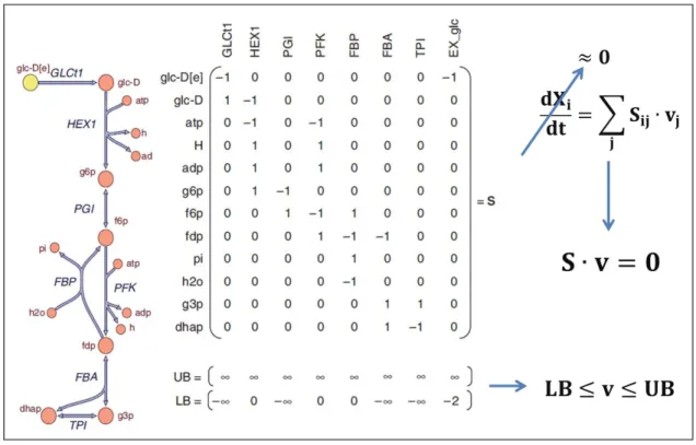
(27) 10. Table 2-1: Computational time spent for the different algorithms in the 3 different computers used, and for the 2 typical types of fermentation: anaerobic batch (AB) and aerobic fed-batch (AF).. Computers used in the study Windows 7 PC, 3.3 GHz AMD FX™ 6100 (6–core) processor Windows 7 PC, 3.1 GHz Intel® Core™ 2 Duo (2–core) processor Linux CentOS 6.4, 2.3 GHz Intel® Xeon® L5640 (6–core) processor. 2.2. dFBA solution. eSS calibration. Pre/post-regression analysis. AB. AF. AB. AF. AB. AF. 7.4 [s]. 31.0 [s]. 7.2 [h]. 13.1 [h]. 14.0 [min]. 51.3 [min]. 7.1 [s]. 28.0 [s]. 6.5 [h]. 12.4 [h]. 13.8 [min]. 49.2 [min]. 6.8 [s]. 25.1 [s]. 4.7 [h]. 13.3 [h]. 11.5 [min]. 41.1 [min]. Metabolic Block. FBA (Orth et al., 2010; Varma & Palsson, 1994) is based on mass balances. As illustrated for a small metabolic network in Figure 2-2, for n reactions and m metabolites a m × n stoichiometric matrix S can be formulated and, if we neglect the accumulation of metabolites – which is reasonable for short periods of time (Stephanopoulos et al., 1998) – a mass balance for all metabolites is: 𝐒∙𝐯=𝟎. (Equation 1). Where v is the flux distribution vector [mmol/gDWh]. Additionally, lower and upper bounds for each flux can be included, based on the reversibility of each reaction (Figure 2-2), along with an objective function to be minimized or maximized, given that the problem is highly subdetermined (i.e. there are much more reactions than metabolites). As previously mentioned, in our approach the metabolic block consists of two sequential optimizations: first, a LP problem is solved by maximizing the specific growth rate (Curran, Crook & Alper, 2012; Hjersted & Henson, 2006; Sohn et al., 2010; Varma & Palsson, 1994):.

(28) 11. 𝐌𝐚𝐱 𝛍 𝐬. 𝐭.. 𝐒∙𝐯 =𝟎. (Problem 1). 𝐋𝐁 ≤ 𝐯 ≤ 𝐔𝐁 Where μ is the specific growth rate [1/h], and LB and UB are the lower and upper bounds, respectively [mmol/gDWh]. Then, a QP problem is applied to minimize the total sum of absolute fluxes (based on the principle of enzyme efficiency maximization (Feng et al., 2012; Holzhütter, 2004; Schuetz, Zamboni, Zampieri, Heinemann & Sauer, 2012)) fixing the growth rate at a sub-optimal level: 𝐌𝐢𝐧 ∑ 𝐯𝐢𝟐 𝐢. 𝐬. 𝐭.. 𝐒∙𝐯 =𝟎. (Problem 2). 𝛍 = 𝛂 ∙ 𝛍∗ 𝐋𝐁 ≤ 𝐯 ≤ 𝐔𝐁 Where μ∗ is the value of the optimal specific growth rate obtained in Problem 1 [1/h], and α is a parameter that varies between 0 and 1 and is used for model calibration (see the Parameter Estimation section). For aerobic cultures, the value of this parameter has one value (α) during the batch stage of the cultivation and another one (αF ) during the fed-batch stage. This is because the fermentation conditions (including the growth rate and the substrate to product yields) change dramatically upon glucose starvation.. The genome-scaled metabolic model used was a version of the consensus model of S. cerevisiae, Yeast 5 (Heavner et al., 2012). We also tried Yeast 6 (Heavner et al., 2013), the most recent version of the consensus model. However, calibrations with our experimental data showed better agreement with Yeast 5 (Table A-1). All FBA problems were solved using the COBRA toolbox (Becker et al., 2007; Schellenberger et al., 2011), which uses the programming library libSBML (Bornstein, Keating, Jouraku & Hucka, 2008) and the SBML toolbox (Keating, Bornstein, Finney & Hucka, 2006). Gurobi® 5.5.

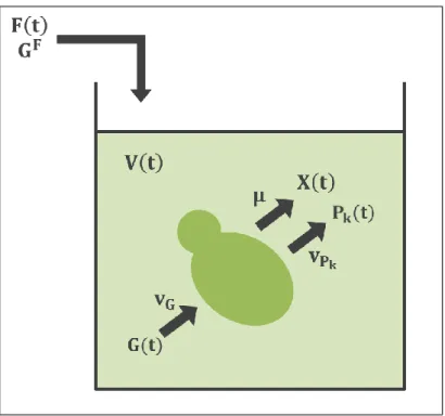
(29) 12. (Gurobi, 2013) was chosen as the optimization solver since preliminary performance tests showed it to be 4 times faster than the default solver. Finally, Gurobi Mex (Yin, 2011) was used as a Matlab-interface for calling Gurobi.. Figure 2-2: Derivation of the FBA equations using a small metabolic network. Adapted from (Becker et al., 2007). 2.3. Dynamic Block. The dynamic block consists of a set of ordinary differential equations (ODEs) that account for volume change, cell growth and metabolite consumption/production, in a batch or fed-batch culture. Figure 2-3 depicts a representation of the fermentation process, in which the state variables (volume, biomass, limiting substrate and products) change in time depending on the feed function and the cell’s specific consumptions and productions..

(30) 13. Figure 2-3: Dynamic system modeled. The vessel represents the bioreactor and the figure inside of it represents yeast. Considering accumulation, entrance, consumption and production, dynamic balances yield the following equations: 𝐝𝐕 𝐝𝐭. = 𝐅(𝐭). 𝐝(𝐕𝐗) 𝐝𝐭 𝐝(𝐕𝐆) 𝐝𝐭. = 𝛍 ∙ (𝐕𝐗). (Equation 3). = 𝐅(𝐭) ∙ 𝐆𝐅 − 𝐯𝐆 ∙ 𝐌𝐌𝐆 ∙ (𝐕𝐗). (Equation 4). 𝐝(𝐕𝐏𝐤 ) 𝐝𝐭. (Equation 2). = 𝐯𝐏𝐤 ∙ 𝐌𝐌𝐏𝐤 ∙ (𝐕𝐗). (Equation 5). Where V is volume [L], t is time [h], F(t) is the feed rate [L/h] (zero for batch cases and exponential for fed-batch cases), X is the biomass concentration [g/L], μ is the specific growth rate [1/h] (obtained from Problem 2 in the metabolic block), G(t) is the extracellular limiting substrate concentration [g/L], GF is the feed’s substrate.

(31) 14. concentration [g/L], Pk is the k-th extracellular product concentration [g/L], v is the corresponding flux exchange rate [mmol/gDWh] (obtained also from Problem 2 in the metabolic block; consumption for substrates and production for products), and MM accounts for the corresponding molecular mass [g/mmol]. All fermentations were carbon-limited, with glucose as the limiting substrate, and ethanol, glycerol, citrate and lactate as the most relevant products. Therefore, Equation 5 comprises 4 differential equations.. The integration solvers were chosen based on preliminary performance tests on all Matlab standard integrators; the best results were achieved with ode113 for batch cultures and ode15s for fed-batch ones. Relative and absolute tolerances of 1e-3 were small enough to obtain good fittings in reasonable computation times. A maximum integration step size of 0.7 h was defined, in order to avoid losing information in critical moments such as glucose starvation. Finally, all variables were forced to be nonnegative. 2.4. Kinetic Block. 2.4.1 Glucose Consumption The kinetic block includes glucose consumption rate (vG ; reaction r_1714 in Yeast 5), defined as a fixed flux (LB = UB) using a Michaelis–Menten kinetic with an additional term to account for ethanol inhibition (Hjersted et al., 2007; Sainz et al., 2003): 𝐯𝐆 =. 𝐯𝐆𝐦𝐚𝐱 𝐆 𝐊 𝐆 +𝐆. ∙. 𝟏 𝟏+. 𝐄 𝐊𝐄. (Equation 6). Where G and E are the glucose and ethanol concentration [g/L] respectively, vGmax is the maximum glucose uptake rate [mmol/gDWh], K G is the half saturation constant [g/L], and K E is the ethanol inhibition constant [g/L]..

(32) 15. 2.4.2 Oxygen Consumption In aerobic fermentations, oxygen uptake rate (vO2 ; reaction r_1992 in Yeast 5) was left unconstrained (LB = −1000 [mmol/gDWh]) during the whole fermentation, because the dissolved oxygen (DO) control guaranteed enough oxygen at any time of the fermentation (Cárcamo et al., 2013). For anaerobic experiments instead, we proceeded as suggested by (Heavner et al., 2012), constraining vO2 to zero (LB = UB = 0 [mmol/gDWh]), allowing unrestricted uptake of ergosterol (r_1757), lanosterol (r_1915), zymosterol (r_2106) and phosphatidate (r_2009), and eliminating 14demethyllanosterol and ergosta-5,7,22,24(28)-tetraen-3beta-ol from the lipid pseudoreaction (in the model this was achieved simply by blocking reaction r_2108 and unblocking reaction r_2109).. 2.4.3 Secondary Metabolite Production Secondary metabolite production was also accounted by forcing the lower bounds of the product exchange reactions to be proportional to glucose consumption. As previously mentioned, the only 4 extracellular products detected in significant amounts were ethanol, glycerol, citrate and lactate; therefore, we included 4 more parameters to calibrate the batch fermentations: 𝐋𝐁𝐢 = 𝐟𝐢 ∙ 𝐯𝐆. ;. 𝐢 = 𝟏…𝟒. (Equation 7). Here, i accounts for (1) ethanol, (2) glycerol, (3) citrate and (4) lactate. LBi is the corresponding exchange reaction lower bound (reactions r_1761, r_1808, r_1687 and r_1546 in Yeast 5, respectively), and fi is the corresponding parameter for calibration. For the aerobic cultivations, these parameters were also allowed to change their value in the fed-batch stage: 𝐋𝐁𝐢 = 𝐯𝐢. ;. 𝐢 = 𝟏…𝟒. (Equation 8).

(33) 16. Where vi are the corresponding extra parameters. This assumption allowed the aerobic simulations to take different yields in batch and fed-batch stages and, moreover, allowed product consumption during glucose-starvation culture conditions, a phenomenon that was observed in some conditions for ethanol and glycerol (see Results and Analysis).. 2.4.4 ATP Maintenance ATP maintenance (mATP ; [mmol/gDWh]) was defined as a minimum consumption flux of cytosolic ATP. Consequently, an additional exchange reaction was added to the metabolic model, which had the following lower bound: 𝐋𝐁𝐀𝐓𝐏[𝐜𝐲𝐭]𝐨𝐮𝐭 = 𝐦𝐀𝐓𝐏. (Equation 9). Here LBATP[cyt]out is the lower bound of the exchange rate of cytosolic ATP, and mATP is a calibrated parameter. mATP accounts for all cellular processes and functions not related to cell growth, i.e. it is the minimum non-growth associated maintenance (NGAM). Growth associated maintenance (GAM), on the other hand, is already included in the biomass pseudo-reaction rate (reaction r_2110 in Yeast 5) and it has a value of 59.3 [mmol/gDWh]. Although we could also include this parameter for calibration and further pre/post regression analysis, it would be strongly correlated with NGAM, and therefore one of the two should be fixed. We choose to focus on NGAM, which can be more easily calibrated considering that it does not directly impact on the biomass pseudo-reaction rate.. 2.4.5 Biomass Requirements Regarding the biomass pseudo-reaction, we considered 3 parameters for calibration that weighted each group of the major cellular requirements differently: a for aminoacids, c for carbohydrates and l for lipids: 𝐚(𝛂𝟏 𝐀 𝟏 + ⋯ + 𝛂𝟐𝟎 𝐀 𝟐𝟎 ) + 𝐜(𝛃𝟏 𝐂𝟏 + ⋯ + 𝛃𝟒 𝐂𝟒 ) + 𝐥(𝛄𝐋) → 𝐁𝐢𝐨𝐦𝐚𝐬𝐬. (Equation 10).

(34) 17. With A1 … A20 being the 20 essential aminoacids; C1 … C4 , the 4 sugars that are part of the biomass pseudo-reaction equation in Yeast 5 ((1->3)-β-D-glucan, glycogen, trehalose and mannan); L, the lipid fraction (obtained from the lipid pseudo-reaction); and α1 … α20 , β1 … β4 and γ, the corresponding stoichiometric coefficients. An important advantage of using this approach for studying sensitivity is that it does not require to evaluate the impact of each compound separately (i.e. every aminoacid, every sugar and every lipid), but instead the impact of each group is assessed. Therefore, one can easily conclude that if one of the 3 parameters does not significantly affect the model’s output, any compound requirement of the corresponding group will neither affect it.. 2.4.6 Gene Expression Finally, two additional parameters were included to account for transcriptomic (gene expression) information. 18 normalized microarray expression datasets (6 for aerobic and 12 for anaerobic cultivations) of different yeast strains were obtained from a published work (Lai, Kosorukoff, Burke & Kwast, 2006) using the query-driven search engine search tool SPELL (Serial Pattern of Expression Levels Locator) (Hibbs et al., 2007) from the Saccharomyces Genome Database (SGD) (Cherry et al., 2012), and from two works from our group (Aceituno et al., 2012; Orellana et al., 2013). All data was preprocessed, disregarding genes that were not included in Yeast 5 or that were essential for biomass growth (using single-knockout gene analysis (Edwards & Palsson, 2000; Zomorrodi, Suthers, Ranganathan & Maranas, 2012)). Overall, 127/119 genes were determined essential for supporting aerobic/anaerobic growth, respectively (Table A-2) and, therefore, were not considered in posterior analyses.. The methodology followed for turning off genes that were not significantly expressed was based on a published method (Åkesson, Förster & Nielsen, 2004). First, depending on the cultivation (aerobic or anaerobic), the corresponding dataset was chosen..

(35) 18. Afterwards, for each gene i and for each microarray j, the binary variable Yij was calculated as: 𝐘𝐢𝐣 = {. 𝟏 ; 𝟎 ;. 𝐞𝐱𝐩𝐢𝐣 ≤ 𝛍𝐣 − 𝐭 𝟏 ∙ 𝛔𝐣 𝐨𝐭𝐡𝐞𝐫𝐰𝐢𝐬𝐞. (Equation 11). Where expij is the normalized expression level of gene i in microarray j, μj is the average expression in microarray j, σj is the corresponding standard deviation, and t1 is a parameter to estimate later and represents an expression threshold. Once all variables Yij were computed, a decision was made for each gene according to the following rule: ∑𝐌 𝐣=𝟏 𝐘𝐢𝐣 ≥. 𝐌∙𝐭 𝟐 𝟏𝟎𝟎. → 𝐆𝐄𝐍𝐢 𝐨𝐟𝐟. (Equation 12). Where M is the number of microarrays in the dataset, and t 2 is another parameter representing a consistency threshold (a minimum percentage in the dataset). Therefore, the expression rule can be summed up as the following: “The i-th gene will be considered unexpressed if in at least t 2 % of the microarrays the expression is t1 standard deviations below the microarray average expression”. If this is true for any gene, then all reactions that are catalyzed by enzymes coded by the corresponding genes will be forced to carry zero flux (LB = UB = 0 [mmol/gDWh]).. Even though gene expression is usually strain-dependent, our approach rests on the premise that if in several gene expression experiments of different yeast strains a particular gene is not expressed over a certain threshold, that gene will probably be unexpressed. in. most. strains. for. that. particular. environmental. condition. (aerobic/anaerobic). Moreover, for simplicity our approach also assumes that each gene will be expressed (or unexpressed) along the whole cultivation. Once again, we overcome this issue by using several microarrays of different strains and different conditions; therefore it is likely that if a gene is not expressed under most of the conditions, it is because it is never expressed during a batch or fed-batch fermentation. It also should be mentioned that the thresholds t1 and t 2 also help to overcome the.

(36) 19. assumptions mentioned, because by calibrating them with experimental data we are obtaining realistic expression rules.. 2.5. Parameter Estimation. For model calibration, we formulated a nonlinear programming problem with the dFBA model as a constraint, and an objective function F consisting of a sum of square errors between the experimental data and the simulation output, weighted by the maximum corresponding measured variable and by the number of measurements of the respective variable: 𝐧𝐢 𝐅 = 𝐌𝐢𝐧 ∑𝐦 𝐢=𝟏 ∑𝐣=𝟏 ( 𝛉. 𝐞𝐱𝐩. 𝐗 𝐦𝐨𝐝 − 𝐗 𝐢𝐣 𝐢𝐣. 𝐞𝐱𝐩. 𝐧𝐢 ∙𝐦𝐚𝐱(𝐗 𝐢𝐣 ). 𝟐. ). (Equation 13). 𝐣. With θ representing the parameter space, m the number of measured variables, ni the number of measurements for the i-th variable, Xijmod the output of the dFBA model for exp. the variable i and the measurement j, and Xij. the experimental value.. All the parameters studied, along with their units, lower and upper bounds and initial values for the optimization are summarized in Table 2-2. The LB and UB of vGmax , K G , K E and mATP were chosen according to the literature (Hjersted et al., 2007; Varma & Palsson, 1994). The UB of fE , fGL , fC and fL were the respective model’s maximum yield from glucose. The LB of t 2 was set at 75%, thus forcing a minimum consistency in the microarray datasets (at least 75% of the datasets have to agree in order to delete a gene). The rest of the LB and UB were chosen to ensure the algorithm had enough search space. Finally, initial values for parameter estimation were chosen to attain a feasible simulation..

(37) 20. Table 2-2: Parameter estimation details. The symbols, names and units of each parameter analyzed in this study are shown. Initial values, lower and upper bounds for parameter estimation are also displayed. Symbol. Name. Units. LB. Initial Value. UB. 𝐯𝐆𝐦𝐚𝐱. Maximum Glucose Uptake Rate. mmol/gDWh. 1. 10. 50. 𝐊𝐆. Half Saturation Constant. g/L. 0.005. 0.05. 10. 𝐊𝐄. Ethanol Inhibition Constant. g/L. 0.005. 20. 50. 𝛂. Sub-Optimal Growth. -. 0.1. 0.7. 1. 𝐚. Aminoacid Requirement. -. 0.5. 1. 3. 𝐜. Carbohydrate Requirement. -. 0.5. 1. 3. 𝐥. Lipid Requirement. -. 0.5. 1. 3. 𝐦𝐀𝐓𝐏. Maintenance ATP. mmol/gDWh. 0. 1. 5. 𝐭𝟏. Expression Threshold 1. -. 0. 6. 6. 𝐭𝟐. Expression Threshold 2. %. 75. 100. 100. 𝐟𝐄. Glucose – Ethanol Minimum Yield. mmol/mmol. 0. 1.7. 2. 𝐟𝐆𝐋. Glucose – Glycerol Minimum Yield. mmol/mmol. 0. 0. 1. 𝐟𝐂. Glucose – Citric Acid Minimum Yield. mmol/mmol. 0. 0. 0.258. 𝐟𝐋. Glucose – Lactic Acid Minimum Yield. mmol/mmol. 0. 0. 1. 𝛂𝐅. Sub-Optimal Growth (fed-batch). -. 0.1. 1. 1. 𝐯𝐄. Ethanol Minimum Rate (fed-batch). mmol/gDWh. -10. 0. 10. 𝐯𝐆𝐋. Glycerol Minimum Rate (fed-batch). mmol/gDWh. -10. 0. 0. 𝐯𝐂. Citric Acid Minimum Rate (fed-batch). mmol/gDWh. 0. 0. 10. 𝐯𝐋. Lactic Acid Minimum Rate (fed-batch). mmol/gDWh. 0. 0. 10. Due to the problem complexity and the presence of multiple local minima, the parameter estimation was performed with the enhanced scatter search method eSS (Egea & BalsaCanto, 2009), which is an improved version of a previous method, SSm (Egea, Rodriguez-Fernandez, Banga & Martí, 2006). SSm (Scatter Search for MATLAB®) is a metaheuristic global optimization algorithm for nonlinear programming problems that has been successfully used in the bioprocess field (Balsa-Canto, Rodriguez-Fernandez & Banga, 2007; Sacher et al., 2011; Sriram, Rodriguez-Fernandez & Doyle, 2012), and obtains a solution expected to be close to the global optimum, using diversification and intensification methods and a reference set of high-quality solutions (Egea et al., 2006). eSS on the other hand uses control vector parameterization (CVP) and is oriented to.

(38) 21. problems with noise and discontinuities (Egea & Balsa-Canto, 2009); therefore, it is ideal for fermentations with substrate limitation and non-constant feed. Additional options should be tuned when using eSS; in our case, the best fittings (lower objective function values in less CPU time) were achieved with a maximum of 3,000 iterations and using the local optimization solver n2fb (Dennis, Gay & Walsh, 1981). With these options, optimization times between 5 and 13 [h] were achieved, depending on the cultivation characteristics and the machine that ran the code (Table 2-1)..

(39) 22. 3. MATERIALS AND METHODS 3.1. Strains and Conditions Assessed. Cultivations were carried out with 2 different strains, the industrial yeast strain S. cerevisiae N30 (Centrovet, Chile) and the wine yeast strain S. cerevisiae EC1118 (Lalvin, Switzerland). For each strain, we tested 4 different environmental conditions:. 1. Aerobic fed-batch with slow feed rate. 2. Aerobic fed-batch with fast feed rate. 3. Anaerobic batch with low glucose initial concentration (G0 ). 4. Anaerobic batch with large glucose initial concentration (G0 ). Since each experiment was done in duplicate, a total of 16 cultivations were performed (4 conditions × 2 strains × 2 duplicates). All media were glucose-limited and completely defined (Table 3-1). Conditions 1, 2 and 3 had G0 = 20 [g/L], whereas condition 4 had G0 = 80 [g/L]. The glucose feed concentration for conditions 1 and 2 was 300 [g/L]. Finally, conditions 3 and 4 were also supplied with ergosterol and Tween 80, both necessary for growth under anaerobic conditions (Diderich et al., 1999), and diluted in a small amount of ethanol..

(40) 23. Table 3-1: Composition of all defined-media employed in this study: batch and feed media for aerobic cultivations, and the 2 different anaerobic batch media used (20 [g/L] and 80 [g/L] of glucose, respectively).. Glucose. Aerobic batch medium 20 g/L. Aerobic feed medium 300 g/L. Anaerobic batch medium (large G0) 80 g/L. Anaerobic batch medium (low G0) 20 g/L. KH2PO4. 6.4 g/L. -. 6.4 g/L. 6.4 g/L. K2HPO4. 450 mg/L. -. 450 mg/L. 450 mg/L. NH4(SO4)2. 5 g/L. -. 5 g/L. 5 g/L. Mg(SO4)∙7H2O. 1 g/L. 5.4 g/L. 4 g/L. 1 g/L. Fe(SO4 )∙7H2O. 4.2 mg/L. 516 mg/L. 16.2 mg/L. 4.2 mg/L. Zn(SO4)∙7H2O. 6.3 mg/L. 24.3 mg/L. 24.3 mg/L. 6.3 mg/L. Cu(SO4)∙7H2O. 420 µg/L. 1.62 mg/L. 1.62 mg/L. 420 µg/L. CaCl2∙2H2O. 286 mg/L. 924 mg/L. 924 mg/L. 286 mg/L. NaCl. 140 mg/L. 300 mg/L. 300 mg/L. 140 mg/L. CoCl2∙6H2O. 420 µg/L. 1.62 mg/L. 1.62 mg/L. 420 µg/L. MnCl2∙4H2O. 1.18 mg/L. 4.54 mg/L. 4.54 mg/L. 1.18 mg/L. H3BO3. 1.4 mg/L. 5.4 mg/L. 5.4 mg/L. 1.4 mg/L. Na2MoO4∙2H2O. 560 µg/L. 2.16 mg/L. 2.16 mg/L. 560 µg/L. KI. 140 µg/L. 540 µg/L. 540 µg/L. 140 µg/L. EDTA. 21 mg/L. 81 mg/L. 81 mg/L. 21 mg/L. d(+)biotin. 600 µg/L. 1.61 mg/L. 1.61 mg/L. 600 µg/L. Ca d(+)panthotenate. 12 mg/L. 32.1 mg/L. 32.1 mg/L. 12 mg/L. Nicotinic acid. 12 mg/L. 32.1 mg/L. 32.1 mg/L. 12 mg/L. Myo-inositol. 300 mg/L. 803 mg/L. 803 mg/L. 300 mg/L. Thiamine Hydrochloride. 12 mg/L. 32.1 mg/L. 32.1 mg/L. 12 mg/L. Pyridoxin Hydrochloride. 12 mg/L. 32.1 mg/L. 32.1 mg/L. 12 mg/L. p-aminobenzoic acid. 2.4 mg/L. 6.42 mg/L. 6.42 mg/L. 2.4 mg/L. Ergosterol. -. -. 40 mg/L. 10 mg/L. Tween 80. -. -. 420 mg/L. 420 mg/L. 3.2. Experimental Setup. The fermenters used for all cultivations consisted of 1 L reactors equipped with a condenser, a stirrer and two Rushton turbines, operating with brushless DC motors VEXTA®, AXH Series (Oriental Motor, Japan). For monitoring and control, a.

(41) 24. SIMATIC PCS7 distributed control system (Siemens, Germany) was used. Dissolved oxygen and temperature were measured with Oxymax COS22D probes (Endress Hauser, Switzerland), pH was detected with Tophit CPS471D probes (Endress Hauser, Switzerland), and off-gas composition (CO2 and O2) was sensed with a BlueInOne Cell gas analyzer (Bluesens, Germany). 210U and 102FS/R peristaltic pumps (Watson Marlow, USA) were used for acid, base, feed and antifoam addition; and FMA–A2407 gas flowmeters and controllers (Omega, USA) for air, O2 and N2 sparged addition. Figure 3-1 displays a photograph of the bioreactor and its main components.. Each culture started from a 2 [mL] vial of the corresponding strain kept at -80°C. A preculture was grown overnight at 30°C in shake flasks with 100 [mL] of the batch medium, from which 50 [mL] for aerobic cultivations (or 60 [mL] for anaerobic cultivations) were inoculated on the 1 [L] fermenters containing 450 [mL] (or 540 [mL], respectively) of batch medium, with controlled conditions of 30°C, pH = 5.0 and whether DO ≥ 2.8 [mg/L] for aerobic cultures, or DO = 0 [mg/L] for anaerobic cultures. Aerobiosis was achieved by a triple split-range action of agitation (300 – 800 [RPM]), air flow (0.2 – 0.6 [L/min]) and pure oxygen flow (0 – 0.6 [L/min]) (Cárcamo et al., 2013), and anaerobiosis was achieved by sparging 0.3 [L/min] of pure nitrogen and agitating at 300 [RPM]. pH was controlled using phosphoric acid 20% [v/v] and ammonium hydroxide 15% [v/v] (the use of the latter also gives additional nitrogen supplementation). Temperature was controlled with a mixture of hot and cold water, using a glass jacket. Lastly, foam was controlled manually using silicone antifoam 10% [v/v]. Figure 3-2 shows the process and instrumentation diagram (P&ID) of the experimental setup..

(42) 25. 1. 4. 2 3 5. 8 6 7. Figure 3-1: Photograph of one of the bioreactors used. Both temperature/oxygen and pH probes are behind the motor and therefore not shown. (1) DC motor connected to the bioreactor agitator. (2) (Filtered) gas entrance to the bioreactor. (3) Condenser. (4) Off gas exit (to CO2 and O2 analyzer). (5) Sampler (behind the condenser). (6) Bioreactor (glass flask inside the glass jacket). (7) Water entrance to the glass jacket. (8) Water exit of the glass jacket..

(43) 26. ARC. ARC. DO. pH. FC. Nitrogen Acid control Oxygen Basic control. Mixer Air. Feed. Antifoam. TRC Sampler Condenser. AT CO2-O2. Off gas. AT DO. AT pH. AR CO2-O2. TT Cool water (10°C) Bioreactor Hot water (50°C). Figure 3-2: P&ID of the system used for all cultivations. Nomenclature used: AT → Analysis Transmitter. AR → Analysis Recorder. ARC → Analysis Recorder & Controller. TT → Temperature Transmitter. TRC → Temperature Recorder & Controller. FC → Flow Controller (Not used in anaerobic conditions). Glucose starvation was detected with a sudden decrease of the CO2 composition in the off-gas, and confirmed each time using Benedict's reagent (Benedict, 1909). For the fedbatch cases (conditions 1 and 2), the feed F(t) was designed for a predefined variable growth rate, and can be calculated from the reactor’s glucose and biomass mass balances, as detailed elsewhere (Villadsen & Patil, 2007): 𝛍. (𝐭). 𝐭. 𝐆𝐗. 𝐢. 𝐅(𝐭) = 𝐆𝐬𝐞𝐭 ∙ 𝐕𝐢 𝐗 𝐢 ∙ 𝐞𝐱𝐩 {∫𝐭 𝛍𝐬𝐞𝐭 (𝐭)𝐝𝐭} 𝐅 ∙𝐘. (Equation 14).

(44) 27. With GF the glucose feed concentration [g/L], YGX the experimental glucose-biomass yield (fixed for Equation 13 in 0.469 [gDW/g] (Møller, Sharif & Olsson, 2004)), t i the time at which the feed started for a given cultivation [h], Vi and Xi the volume [L] and biomass [g/L] values at t i , respectively, and μset (t) the variable growth rate. The latter was defined as the following: 𝛍𝐬𝐞𝐭 (𝐭) = 𝐀 + 𝐁 ∙ 𝐞−𝐂𝐭. (Equation 15). Where A and B are both 0.07 [1/h] for all aerobic cultivations, and C is 0.14 [1/h] for condition 1, and 0.07 [1/h] for condition 2. Therefore, μset (t) decays more quickly in. 0.14. 0.004. 0.13. 0.0035. 0.12. 0.003. 0.11. 0.0025. 0.1. 0.002. µ(set), C = 0.14 [1/h]. 0.09. F [L/h]. µ(set) [1/h]. condition 1, which translates into a slower feed rate (Figure 3-3).. 0.0015. µ(set), C = 0.07 [1/h] F, C = 0.14 [1/h]. 0.08. 0.001. F, C = 0.07 [1/h] 0.07. 0.0005 0. 2. 4. 6. 8. 10. t [h]. Figure 3-3: The temporal evolutions of the design growth rate (µset) and a given feed rate (F) for experimental conditions 1 (C = 0.14 [1/h]) and 2 (C = 0.07 [1/h]) are displayed, with t = 0 as the feed starting point. Condition 1 has a quicker decay in µset than condition 2, and therefore has a slower F than condition 2. For F visualization, typical experimental conditions were selected: Vi = 0.4 [L] and Xi = 4 [g/L] (for further details refer to Equation 14)..

(45) 28. 3.3. Assay Methods. Samples of ~5 [mL] were taken periodically from all cultivations. Biomass was measured in OD using a UV-160 UV-visible recording spectrophotometer (Shimadzu, Japan), and results were transformed to g/L using a calibration curve of 0.3797 [gDW/L/OD] for the N30 strain and of 0.3840 [gDW/L/OD] for the EC1118 strain (both determined with an infrared dryer-equipped balance (Precisa, Switzerland)).. A 2 [mL] aliquot of each sample was centrifuged for 5 minutes at 14,000 RPM and 4°C, using a Mikro 22R centrifuge (Hettich, Germany). All supernatants were kept at -80°C until the fermentation was over. Extracellular metabolites were afterwards measured by high-performance liquid chromatography (HPLC) in duplicate. 100 [µL] of a solution 27.5 [mM] H2SO4 and with 16.7 [g/L] of pivalic acid (used as internal standard) were added to 1 [mL] of each sample and each of the HPLC standards (with known concentrations of trehalose, glucose, fructose, glycerol, ethanol, citrate, malate, succinate, lactate and acetate). Afterwards, 20 [µL] of the resulting solutions were injected into a LaChrom L-7000 HPLC system (Hitachi, Japan), with an Aminex HPX87H anion-exchange column (Bio-Rad, USA) for organic acids, alcohols and sugars separation, working at 55°C with a 0.5 [mL/min] flow of mobile phase 2.5 [mM] H 2SO4 (the same concentration as the one in each sample after adding the internal standard solution). A LaChrom L-7450A diode array detector (Hitachi, Japan) was used at 210 [nm] for detecting organic acids, and a LaChrom L-7490 refraction index detector (Hitachi, Japan) for sugars and alcohols. Finally, each metabolite was quantified normalizing each area in the chromatogram by the corresponding internal standard area and using a calibration curve with the HPLC standards..

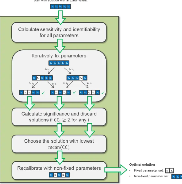
(46) 29. 3.4. Reparameterization Analysis. 3.4.1 General Methodology of Procedure As mentioned in the introduction, we used a novel methodology to obtain a set of identifiable and significant parameters in our dFBA model for each of the 16 experimental cultivations. As shown in Figure 3-4, the methodology starts by calculating sensitivity and identifiability for the estimated parameters of the calibration. Then, the parameters are iteratively fixed: At the end of each iteration, and depending on the regression diagnostics result, a parameter is eliminated (thus its value becomes fixed) for the next iteration. The following rules were considered for deciding which parameters to fix (for further details of each analysis see the Pre/Post Regression Diagnostics section):. 1. Identifiability: when 2 parameters had a Pearson correlation coefficient larger than 0.95, different combinations of the corresponding estimated values resulted in the same objective function in the parameter estimation procedure and, consequently, the decision was to fix at least one of them. 2. Sensitivity: when the relative sensitivity of a parameter was below 0.01 for all variables, the parameter was considered to have no influence in the model, and therefore was decided to be fixed.. For most of the iterations, more than one of the above problems will arise, and therefore exploratory branches for each of the corresponding parameters are necessary, which generates a growing exploratory tree. However, because the procedure could generate an excessive number of branches, model-specific policies should be defined in order to overcome this issue. Our aim here was to find an adequate set of parameters for our model with reasonable computational times. In this work, the main strategy to reduce the exploratory tree size was to count the number of problems (identifiability and sensitivity) for each parameter at each round of the procedure. If any parameter had both problems, exploratory branches were created only for the parameters with the 2.

(47) 30. problems. On the other hand, if there were only parameters with 1 of the 2 problems, we created branches for all the problematic parameters. Finally, if no parameter had any of the mentioned problems, the solution was saved for posterior analyses, and the branch no longer explored.. Figure 3-4: Methodology used in this study for obtaining dFBA models with sensitive, uncorrelated and significant parameters. As an example, a solution with 5 parameters is analyzed..

(48) 31. Once the exploratory tree concluded, the combinations that showed no identifiability or sensitivity problems were collected, and confidence coefficients (CCs) were calculated for each non-fixed parameter (Figure 3-4). The CCs had to be calculated for each of the combinations, given that their values are dependent on the combination of estimated parameters, in contrast with the sensitivity and correlation values, which remain constant regardless of the combination of estimated parameters (and therefore could be calculated only at the beginning of the procedure). If any non-fixed parameter from a solution had a CC larger than 2, it was considered that the parameter had a value not significantly different from zero, and therefore the corresponding solution was disregarded.. Finally, for each of the 16 experimental conditions, the solution with the smallest mean CC was chosen as the optimal reparameterization (Figure 3-4). This solution had a fixed parameter set (i.e. parameters eliminated by the procedure) and a non-fixed parameter set (i.e. parameters used for model calibration). To further improve the results, each of these 16 solutions were used to repeat the parameter estimation, but only with the corresponding non-fixed parameter set; the fixed parameter set had the same values than the originally estimated ones.. 3.4.2 Pre/Post Regression Diagnostics In the following, we will briefly explain the regression diagnostics used in this study, as it has been thoroughly presented elsewhere (Jaqaman & Danuser, 2006; Sacher et al., 2011). Sensitivity analysis accounts for the relative impact that each parameter has in each of the model’s state variables. In our approach, we computed the relative sensitivity (Gik ), as indicated: 𝛉. 𝐝𝐗 𝐢 (𝐭). 𝐢. 𝐝𝛉𝐤. 𝐤 𝐆𝐢𝐤 (𝐭, 𝛉𝐤 ) = 𝐗 (𝐭). (Equation 16). Where t is time, θk is the k-th parameter and Xi (t) is the i-th variable at time t. With all Gik values, for each time we formed a sensitivity matrix G(t), in which the k-th column.

(49) 32. denotes the sensitivity of the k-th parameter on the state variables. In order to obtain a single normalized score (spanning all experimental times) of each parameter over each variable, we calculated average sensitivity as detailed in (Hao, Zak, Sauter, Schwaber & Ogunnaike, 2006). Therefore, if this score is under 0.01 in each variable for a given parameter, we chose to fix the corresponding parameter.. For identifiability calculations, the MATLAB function corrcoef was used to calculate the correlation coefficients between each column of the sensitivity matrices, and stored the information in a correlation coefficients matrix (C). If any of the matrix absolute values (besides the diagonal) is over a certain threshold (in our case |Cij| ≥ 0.95), both of the associated parameters are strongly correlated, and therefore one of both should be fixed.. For significance calculations, and also using the sensitivity matrices, we first calculated the Fisher Information Matrix (FIM) (Petersen, Gernaey & Vanrolleghem, 2001): 𝐅𝐈𝐌 = ∑𝐧𝐣=𝟏 𝐆𝐣𝐓 𝐐𝐣 𝐆𝐣. (Equation 17). Here, Gj is the sensitivity matrix for measurement j, n is the number of measurements, and Qj is the inverse of the measurement error covariance matrix assuming white and uncorrelated noise, which is used as a weighting matrix. Using this matrix, the variances for each estimated parameter (σ2k ) were calculated as (Landaw & DiStefano III, 1984; Petersen et al., 2001): −𝟏 𝛔𝟐𝐤 = 𝐅𝐈𝐌𝐤𝐤. (Equation 18). With the variances we computed the confidence interval (CI) with 5% significance for the k-parameter as follows: ̂𝐤 ± 𝟏. 𝟗𝟔 𝛔𝐤 ] 𝐂𝐈𝐤 = [𝛉. (Equation 19). Where θ̂k is the estimated value of the respective parameter. Finally, coefficients of confidence (CC) were calculated as follows:.

(50) 33. 𝐂𝐂𝐤 =. ∆(𝐂𝐈𝐤 ) ̂𝐤 𝛉. (Equation 20). With ∆(CIk ), the CI’s length. With this metric, we determine that a parameter is not significantly different from zero if the CI contained the zero, therefore if the corresponding CC was larger than 2.. The duration to compute the whole aforementioned pre/post regression diagnostics lasted between 10 and 50 [min], depending on the experimental conditions and the computer employed (Table 2-1).. 3.4.3 Cross-Calibration Once the reparameterization was performed for each of the 16 cultivations, the consistency of each solution was studied by performing a cross-calibration between the cultivations. Both the fixed and non-fixed parameter sets obtained from each fermentation were used to calibrate the remaining 7 fermentations (aerobic or anaerobic), i.e. fixing the corresponding parameters with the fixed parameter set values and fitting the data with the non-fixed parameter set. Afterwards, a cross calibration coefficient (CCC) was computed as: 𝐅. 𝐂𝐂𝐂𝐢𝐣𝐤 = 𝐅𝐢𝐣𝐤 𝐣𝐣𝐤. ;. 𝐢, 𝐣 = 𝟏 … 𝟖 ; 𝐢 ≠ 𝐣 ;. 𝐤 = {𝟎, 𝟏} (Equation 21). Where Fijk is the objective function obtained with the i-th solution using the experimental data of the j-th cultivation, and k is an index for distinguishing between aerobiosis (k = 1) and anaerobiosis (k = 0). Therefore, if the CCCijk is close to 1, the ith solution used to calibrate the j-th experimental data is appropriate. On the other hand, if CCCijk is much larger than 1, a good fit was not possible and therefore the i-th solution is not useful for predicting different experimental conditions..