TÍTULO
BRAZIL
A POSSIBLE SYMBIOTIC RELATIONSHIP BETWEEN THE
EVOLUTION OF CARBON EMISSIONS, ENERGY CONSUMPTION
AND ECONOMIC GROWTH
AUTORA
Erika Reesink Cerski
Esta edición electrónica ha sido realizada en 2017
Tutores PhD. José Enrique García Ramos ; PhD. Ángel Mena Nieto Instituciones Universidad Internacional de Andalucía ; Universidad de Huelva
Curso Máster Oficial Interuniversitario en Tecnología Ambiental
ISBN 978-84-7993-765-2
Erika Reesink Cerski
De esta edición: Universidad Internacional de Andalucía
Fecha
Reconocimiento-No comercial-Sin obras derivadas
Usted es libre de:
Copiar, distribuir y comunicar públicamente la obra.
Bajo las condiciones siguientes:
Reconocimiento. Debe reconocer los créditos de la obra de la manera. especificada
por el autor o el licenciador (pero no de una manera que sugiera que tiene su apoyo o apoyan el uso que hace de su obra).
No comercial. No puede utilizar esta obra para fines comerciales.
Sin obras derivadas. No se puede alterar, transformar o generar una obra derivada
a partir de esta obra.
Al reutilizar o distribuir la obra, tiene que dejar bien claro los términos de la licencia
de esta obra.
Alguna de estas condiciones puede no aplicarse si se obtiene el permiso del titular
de los derechos de autor.
1
THE INTERNATIONAL UNIVERSITY OF ANDALUCIA
THE UNIVERSITY OF HUELVA
BRAZIL: A POSSIBLE SYMBIOTIC RELATIONSHIP BETWEEN THE
EVOLUTION OF CARBON EMISSIONS, ENERGY CONSUMPTION AND
ECONOMIC GROWTH.
MASTER THESIS PRESENTED BY
ERIKA REESINK CERSKI
IN THE POSTGRADUATE PROGRAM IN ENVIRONMENTAL TECHNOLOGY
ADVISORS
PhD. JOSÉ ENRIQUE GARCÍA RAMOS PhD. ÁNGEL MENA NIETO
“Scientific evidence for warming of the climate system is unequivocal,
there is 95 percent confidence that humans are the main cause of the
current global warming”.
- Intergovernmental Panel on Climate Change
"La evidencia científica para el calentamiento del sistema climático es
inequívoca, hay 95 por ciento de confianza que los seres humanos son la
principal causa del calentamiento global actual".
3
Acknowledgments
I would like to thank my advisors, José Enrique García Ramos and Ángel Mena Nieto, whose work showed me that concern for environmental affairs, supported by an “engagement” in literature and technology, should always consider an interaction of not only environmental, but also social, economic, political and cultural factors in order to provide alternatives for our times.
I would also like to thank Fundación Carolina for their financial support granted to Latin America students, which allowed me to have this stunning experience of taking my Master’s at both the International University of Andalucia (UNIA) and the University of Huelva (UHU).
Furthermore, I would like to thank the city of Huelva, especially La Rabida, for its warm and friendly welcome. And for giving me the opportunity to make friends and share experiences, which I will take with me for the rest of my life.
ABSTRACT
In December 2015, 195 countries adopted the first-ever legally binding global climate deal at Paris Climate Conference (COP21), known as Paris Agreement. Although, the agreement entered into force on November 4th in 2016, it sets out a global action plan to avoid risky climate change by limiting global warming less than to 2°C in the long term. In the Paris Agreement, Brazil plays a crucial role due to the fact that it has the ninth largest economy in the world, an important relationship with its neighbors in South America, a population exceeding 200 million people, and covers practically the entire Amazon Rainforest. These are some of the reasons that explain why Brazil has pledged to cut down greenhouse gases (GHG) emissions by 37 per cent by 2025, and 43 per cent by 2030, compared to 2005 levels.
The development of a country, especially Brazil, requires appropriate and realistic policies to current and changing demands. In this way, it is fundamental to achieve not only a secure but also a consistent environmental planning for the energy sector and GDP growth. Within this context, this study proposes a model of economic growth, carbon emissions and sustainable development for Brazil.
This work applies to the period 1971-2030, using the methodology proposed by Robalino-López (2014), based on a GDP formation approach, which includes the effect of renewable energies. A historical data, from 1971 to 2012, and a forecast period of 18 years have been considered for testing four different economic scenarios. Our predictions show that the scenario which corresponds to a heavy GDP increase can have the same value of CO2 emissions as a scenario in which the GDP increases
5
RESUMEN
En diciembre de 2015, 195 países adoptaron un acuerdo climático universal y jurídicamente vinculante en Paris, conocido como Acuerdo de París sobre Cambio Climático y que nació en la Conferencia del Clima de París (COP21), aunque no ha entrado en vigor hasta el 4 de noviembre de 2016. El acuerdo establece un plan de acción global para evitar el peligroso Cambio Climático, y limita el calentamiento global por debajo de 2°C. Brasil tiene un papel crucial en el Acuerdo de París, pues es la novena economía del mundo, tiene una importante relación con sus países vecinos en América del Sur, tiene una población actual de 200,4 millones de personas y cubre casi toda la Amazonía. Estas son algunas de las razones que explican por qué Brasil se ha comprometido a reducir las emisiones de gases de efecto invernadero en un 37 por ciento en 2025, y en un 43 por ciento en 2030, en comparación con los niveles de 2005. El desarrollo de un país, especialmente del Brasil, requiere políticas adecuadas y realistas a las demandas actuales y futuras. De esta manera, es fundamental tener una planificación segura y consistente, pero también ecológica para el sector energético y el crecimiento del PIB.
Dentro de este contexto, el presente estudio propone un modelo que englobe el crecimiento económico, las emisiones de carbono y el desarrollo sostenible de Brasil. Este trabajo analiza el período 1971-2030, utilizando la metodología propuesta por Robalino-López (2014), para estudiar el efecto del uso de las energías renovables sobre la formación del PIB. Un período histórico de 1971 a 2012 y una previsión de 18 años han sido considerados en la prueba de cuatro diferentes escenarios económicos y energéticos.Nuestras predicciones muestran que el escenario que corresponde a un fuerte aumento del PIB puede tener el mismo valor de emisiones de CO2 que un
List of Figures
Figure 1. Schematic plot of the relationship between the GDP per capita (pc) and the CO2 emission per capita: (1) linear growth of the emission, (2) stabilization, and (3) reduction of the
CO2 emission as the income increases ... 11
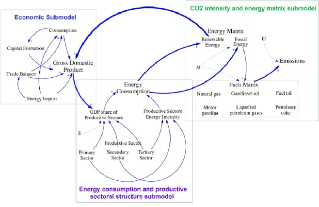
Figure 2. Causal diagram of the model. Continuous lines stand for the relationship between variables, while dashed ones correspond to control terms(S: productive sectoral structure, M: energy matrix, U: emission factors). Bold line represents a feedback mechanism.. ... 25
Figure 3. Domestic electricity supply by source ... 31
Figure 4. Domestic electricity supply by sector. ... 32
Figure 5. Domestic energy supply in 2014. ... 34
Figure 6. Evolution of the domestic energy supply structure. ... 35
Figure 7. GDP official and predicted data. ... 49
Figure 8. Fossil energy official and predicted data. ... 50
Figure 9. Renewable energy official and predicted data. ... 50
Figure 10.Total energy official and predicted data. ... 50
Figure 11.CO2 emissions official and predicted data. ... 51
Figure 12. GDP of Brazil for the period 1971-2011. ... 53
Figure 13. GDP of Brazil for the period 2010-2030. ... 53
Figure 14. Total energy consumption of Brazil for the period 1971-2011 ... 54
Figure 15. Total energy consumption of Brazil for the period 2010-2030. ... 55
Figure 16. Fossil energy consumption of Brazil for the period 1971-2030. ... 55
Figure 17. Renewable energy consumption of Brazil for the period 1971-2030. ... 56
Figure 18. Energy consumption of Brazilian primary sector for the BS and SC-2 scenarios during the period 2000-2030... 56
Figure 19. Energy consumption of Brazilian primary sector for the SC-3 and SC-4 scenarios during the period 2000-2030. ... 57
Figure 20. Energy consumption of Brazilian manufacturing sector for the BS and SC-2 scenarios during the period 2000-2030. ... 58
Figure 21. Energy consumption of Brazilian manufacturing sector for the SC-3 and SC-4 scenarios during the period 2000-2030. ... 58
Figure 22. Energy consumption of Brazilian energetic sector for the BS and SC-2 scenarios during the period 2000-2030. ... 59
Figure 23. Energy consumption of Brazilian energetic sector for the SC-3 and SC-4 scenarios during the period 2000-2030. ... 59
Figure 24. Energy consumption of Brazilian tertiary sector for the BS and SC-2 scenarios during the period 2000-2030... 60
Figure 25. Energy consumption of Brazilian tertiary sector for the SC-3 and SC-4 scenarios during the period 2000-2030. ... 61
7
Figure 27. Brazilian energy consumption of natural gas for the four scenarios for the period
2010-2030. ... 62
Figure 28. Brazilian energy consumption of liquefied petroleum gases for the four scenarios for the period 2010-2030... 63
Figure 29. Brazilian energy consumption of motor gasoline for the four scenarios for the period 2010-2030. ... 63
Figure 30. Brazilian energy consumption of gas/diesel oil for the four scenarios for the period 2010-2030. ... 64
Figure 31. Brazilian energy consumption of fuel oil for the four scenarios for the period 2010-2030. ... 64
Figure 32. Brazilian energy consumption of petroleum coke for the four scenarios for the period 2010-2030. ... 65
Figure 33. Brazilian consumption of renewable, alternative and nuclear energies for the four scenarios for the period 2010-2030. ... 66
Figure 34. CO2 emissions of Brazil for the period 1971-2011. ... 67
Figure 35. CO2 emissions of Brazil for the period 2010-2030. ... 67
List of Tables
Table 1. Summary of recent studies that analyzed the GDP growh-energy-CO2 relationship. ... 14Table 2. Default CO2 emission factors for combustion. ... 23
Table 3. Brazilian total population from 2000 to 2060. ... 29
Table 4. Domestic energy supply from 2005 to 2014 ... 34
Table 5. Brazilian general data. ... 38
Table 6. Brazilian general data. Part II... 39
Table 7. Information about Brazilian agriculture sector. ... 40
Table 8. Information about Brazilian manufacturing sector. ... 41
Table 9. Information about Brazilian energetic sector. ... 42
Table 10. Information about Brazilian tertiary sector. ... 43
Table 11. Energy by type of fuels in agriculture sector. ... 44
Table 12. Energy by type of fuels in imanufacturing sector. ... 45
Table 13. Energy by type of fuels in energetic sector. ... 46
Table 14. Energy by type of fuels in tertiary sector. ... 47
List of Acronyms
BERC Brazilian Energy Research Company (Empresa de Pesquisa Energética-EPE) BIGS Brazilian Institute of Geography and Statistics (Instituto Brasileiro de
Geografia e Estatística-IBGE)
CH4 Methane
CO2 Carbon Dioxide
CO2eq Carbon Dioxide Equivalent COP21 Paris Climate Conference
EKC Environmental Kuznets Curve
FRB Federative Republic of Brazil (República Federativa do Brasil)
GDP Gross Domestic Product
GHG Greenhouse Gas
Gt Gigatonne
GtCO2eq Gigatonne Carbon Dioxide Equivalent
GWh Gigawatt Hour
ICLFS Integrated Cropland-livestock-forestry Systems
HDI Human Development Index
iNDC Intended Nationally Determined Contribution IPCC Intergovernmental Panel on Climate Change
kWh Kilowatt Hour
ME Ministry of the Environment (Ministério do Meio Ambiente- MMA)
Mt Million Tonnes
MW Megawatt
NAEE National Agency of Electric Energy
N2O Nitrous Oxide
PPP Purchasing Power Parity
toe Tonne of Oil Equivalent
ton Tonne
TWh Terawatt Hour
UNDP United Nations Development Program UNEP United Nations Environment Programme
UNESCO United Nations Educational Scientific and Cultural Organization UNFCCC United Nations Framework Convention on Climate Change
USD United States Dollar
9
CONTENTS
1. INTRODUCTION ... 10
1.1. The goals of this research ... 13
2. LITERATURE REVIEW ... 14
3. MODEL AND METHODOLOGY ... 19
3.1 Formulation of the model ... 19
3.2 Economic submodel ... 21
3.3 Energy consumption and productive sectoral structure submodel ... 22
3.4 CO2 intensity and energy matrix submodel ... 22
3.5 Model equations and causal diagram ... 25
3.6 Model validation and verification ... 26
4. RESULTS AND DISCUSSION ... 28
4.1 Brazil in numbers ... 28
4.1.1 Overview ... 28
4.1.2. Economy ... 29
4.1.3 Energy analysis ... 30
4.1.4 Forecasts for 2030 ... 34
4.1.5. Brazil and the United Nations Framework Convention on Climate Change ... 36
1. INTRODUCTION
According to Intergovernmental Panel on Climate Change (IPCC, 2014), despite a growing number of climate change mitigation policies, annual greenhouse gas (GHG) emissions grew on average by 1.0 gigatonne carbon dioxide equivalent (GtCO2eq)
(2.2%) per year from 2000 to 2010 compared to 0.4 GtCO2eq (1.3%) per year from
1970 to 2000. The highest anthropogenic GHG emissions in human history were from 2000 to 2010, which reached 49 (±4.5) GtCO2eq/yr in 2010. Besides, CO2 emissions
from fossil fuel combustion and industrial processes contributed about 78% of the total GHG emission increase from 1970 to 2010. In addition, CO2 remained the major
anthropogenic GHG accounting for 76% of the total emissions in 2010, 16% coming from methane (CH4), 6% from nitrous oxide (N2O), and 2% from fluorinated gases.
Globally, economic and population growth are continued to be the important drivers in CO2 emissions derived from fossil fuel combustion. The contribution of
population growth between 2000 and 2010 remained similar to the previous three decades, whereas the contribution of economic growth rose sharply. Anthropogenic GHG emissions are mainly driven by population size, economic activity, lifestyle, energy use, land use patterns, technology and climate policy (IPCC, 2014).
Several international organizations have been warning about the need of stabilizing CO2 and other anthropogenic GHG emissions in order to avoid catastrophic
11
Unfortunately, the economic growth, according to the environmental Kuznets curve (EKC), in a first stage will also increase the CO2 emissions of the country. The EKC
reveals how a technically specified environmental quality measurement changes according to the income of a country (see Figure 1).
Figure 1. Schematic plot of the relationship between the GDP per capita (pc) and the CO2 emission per capita: (1) linear growth of the emission, (2) stabilization, and (3) reduction of the
CO2 emission as the income increases. Source: Robalino-López et al., 2014.
between level of economic activity and environmental pressure (defined as the level of concentration of pollution or flow of emissions, depletion of resources, etc.).
The decomposition of changes in an aggregate environmental impact and of its driving forces has become popular to unravel the relationship of society and economy with the environment. The specific application in energy consumption and CO2
emissions is known as Kaya identity (Kaya, 1990 and Kaya et al., 1993). The Kaya identity is a linking expression of factors that determine the level of human impact on environment, in the form of CO2 emissions. It states that total emission level can be
expressed as the product of four inputs: population, GDP per capita, energy use per unit of GDP, carbon emissions per unit of energy consumed. The Kaya identity plays a core role in the development of future emissions scenarios in the IPCC Special Report on Emissions Scenarios (IPCC, 2000). The scenarios set out a range of assumed conditions for future development of each of the four inputs. Population growth projections are available independently from demographic research; GDP per capita trends are available from economic statistics and econometrics; similarly for energy intensity and emission levels. The projected carbon emissions can drive carbon cycle and climate models to predict future CO2 concentration and climate change.
The identification of these kinds of sources of CO2 emissions and of their
magnitude is essential information for economic planning and decision makers. As Chien and Hu (2008) and Robalino-López et al. (2013, 2014) had shown the use of renewable energy improves the CO2 efficient emission in relation to economic growth.
13
1.1. The goals of this research
The general objective of this research is to estimate the CO2 emissions in Brazil
using and improving the Robalino-López (2014) methodology; the research also aims to understand the driving forces that guide the emission process, such as economic growth, energy use, energy structure mix, and fuel use in the productive sectors.
A multi-scenario approach is used to analyze the evolution of energy consumption and energy-related emissions and its implications in the socio-economic and environmental development of the study area.
This study could help the development and implementation of proactive policies to the challenge of sustainable development. The application of scenario analysis-modelling in the short-to-medium term is intended to develop insights into plausible future changes with green goals in the driving forces of the national policies. The specific research objectives are:
To study in details the way that changes in the energy matrix and in gross domestic product (GDP) will affect CO2 emissions in the country.
To develop a set of integrated qualitative and quantitative baseline scenarios at both macro and sectorial level to explore plausible alternative development of income, energy use and CO2 emissions in a
medium term (2030) in Brazil.
To fill the gap in the literature of studies on the relationship between emissions, energy consumption and income growth in Brazil.
2. LITERATURE REVIEW
In this day and age, sustainable development it is a very popular topic. Many countries, regardless to their economic situation, have been studying the relationship between economic growth, energy consumption and CO2 emission. In the literature it
is possible to find many researches about this subject, as shown on Table 3, which summarizes the set of references, analyzed in detail below. Notice that there are different lines of research, some study the relationship between GDP and energy consumption or GDP, energy and CO2 emissions, including the study of the causality
relationships; others study the different aspects of the EKC hypothesis; and finally, there are also researches that use scenarios to be able to conduct forecast calculations of CO2 emissions in forthcoming period.
Table 1. Summary of recent studies that analyzed the GDP growh-energy-CO2 relationship.
Author Relationship Region Methodology Period Outcomes Padilla et al. CO2-GDP Groups of
Kuntsi-Reunanen CO2-energy Selected Latin America
BRICS countries Granger causality 1990-2010
Evidences of GDP → CO2
Ibrahim et al. CO2-GDP 69 countries GMM estimators 2000-2008
Mixed evidences
15
Padilla et al. (2006) researched the inequality in C02 emissions across group of
countries and the relationship with the income inequality from 1971 to 1999. The authors concluded that for an overwhelming majority of countries, higher per capita income should be expected to be followed by higher emissions.
In 2007 Kuntsi-Reunanen studied a comparison of Latin America energy with CO2 emissions from 1970 to 2001. The author inferred that the increase in CO2
emissions could be attributed partly to economic growth and to population growth. Also, the structural shifts from a rural, predominantly agricultural economic base, to a manufacturing one resulted in increasing energy demand. As Winkler et al. (2002) affirmed the nature of the energy economy will strongly influence emissions per capita of GDP. Kutsi as well concluded that since the developing countries will continue to emphasize their manufacturing sectors, CO2 emissions can be expected to increase
unless energy efficiency is increased commensurably. While energy efficiency has slightly improved in these countries, the improvement is considerably lower than countries of the Organisation for Economic Co-operation and Development (OECD). Most developing countries should be expected to increase their emissions to meet human development needs at least in the next few decades.
Narayan and Narayan (2010) explored the carbon dioxide emissions and economic growth from 43 developing countries in the period 1980 to 2004. A new approach was employed. They propose that if the long-run elasticity is lower than the short run elasticity, then this is also equivalent to lower carbon emissions as economic growth occurs over time. With this methodology, they found that in 35% of the sample the CO2 diminished in the long run, which confirms that these countries approach the
sloping down part of the EKC.
Jaunky (2011) attempted to examine the EKC hypothesis for 36 high income countries over the period 1980–2005. The author applied the methodology proposed by Narayan and Narayan (2010) and added several panel unit root and co-integration tests. He detected unidirectional causality, running from GDP to CO2 emissions, in
short-run and long-run. In the long-run, CO2 emissions have fallen as income rises for
Robalino-López et al. (2013, 2014) presented a model approach of CO2
emissions in Ecuador up to 2020 and also analyzed whether the EKC hypotheses holds within the period 1980-2025 under four different scenarios. The main goal was studied in detail the way the changes in the energy matrix and in the GDP would affect the CO2
emissions of the country. In particular, the effect of a reduction of the share of fossil energy, as well as of an improvement in the efficiency of the fossil energy use. The results do not supported the fulfillment of the EKC, nevertheless, its showed that it is possible to control the CO2 emissions even under a scenario of continuous increase of
the GDP, if it is combined with an increase of the use of renewable energy, with an improvement of the productive sectoral structure and with the use of a more efficient fossil fuel technology.
Cowan et al., in 2014, studied the nexus of electricity consumption, economic growth and CO2 emissions in the BRICS countries from 1990 to 2010. The results
suggest that the existence and direction of Granger causality differ among the different BRICS countries. The main recommendation for these countries in general is to increase investment in electricity infrastructure. Because, this will expand electricity production capabilities in order to keep up with supply, while at the same time improving electricity efficiency. This will result in higher levels of electricity production and lower levels of CO2 emissions.
However, in terms of Brazil, Cowan et al. (2014) concluded that no evidence of causality running in any direction between electricity consumption and economic growth is found, thus supporting the neutrality hypothesis. Similarly, no causality was found to exist between electricity consumption and CO2 emissions. This result makes
sense as electricity only accounts for a marginal amount of Brazil's total GHG emissions, the majority coming from land usage. This relatively small contribution made by the electricity sector may also be a result of increasing levels of infrastructure and the use of renewable energy sources, particularly hydroelectricity in Brazil. With respect to the CO2 emissions—economic growth nexus, causality was found to run
from CO2 emissions to economic growth. This result may be due to the rapid and
17
agriculture and the resulting employment have helped to increase economic growth but at the expense of raising CO2 levels, not just in Brazil, but globally.
Ibrahim and Law (2014) examined the mitigating effect of social capital on the EKC for CO2 emissions using a panel data of 69 developed and developing countries.
Adopting generalized method of moments (GMM) estimators, they found evidence substantiating the presence of EKC. Moreover, the authors suggest that the pollution costs of economic development tend to be lower in countries with higher social capital reservoir. In addition to policy focus on investments in environmentally friendly technology and on the use of renewable energy, investments in social capital can also mitigate the pollution effects of economic progress.
Al-mulali et al. (2014) investigated the impact of electricity consumption from renewable and non-renewable sources on economic growth in 18 Latin American countries between 1980 and 2010. It was found that economic growth, renewable electricity consumption, non-renewable electricity consumption, gross fixed capital formation, total labor force and total trade were cointegrated. In addition, the results revealed that renewable electricity consumption, non-renewable electricity consumption, gross fixed capital formation, total labor force, and total trade have a long run positive effect on economic growth in the investigated countries. The most important conclusion is that electricity consumption from renewable sources is more effective in increasing the economic growth than the nonrenewable electricity consumption in the investigated countries.
Robalino-López et al., in 2015, tested the case of Venezuela for the period 1980-2025, through a methodology based on an extension of Kaya identity and on a GDP formation approach that includes the effect of renewable energies, the same that will be used in this work. Also the authors experimented the EKC hypothesis under different economic scenarios. The predictions showed that Venezuela does not fulfill the EKC hypothesis, however, the country could be on the way to achieve environmental stabilization in the medium term.
Later Robalino-López et al. (2016) analyzed the convergence process in CO2
South American countries (Argentina, Bolivia, Brazil, Chile, Colombia, Ecuador, Peru, Paraguay, Uruguay and Venezuela). They concluded that over these countries Brazil has the highest GDP in the region reaching 1968 billion USD in 2010, and that Brazilian industry is the most energy demanding sector of these countries. Furthermore, the results show that energy intensity in South America is lower (136 kgoe/000 USD in 2010) than world average energy intensity (184 kgoe/000 USD). However, the CO2
intensity (CO2 over energy) in the region has remained relatively constant (2.2 kg
CO2/kgoe) during the analyzed period and always below the world average (2.5 kg
CO2/kgoe). In addition, the use of renewable energy is very heterogeneous in the
region. Indeed, the share of renewable and alternative energy in the total energy use is (for the year 2010): 6.0% for Argentina, 2.5% for Bolivia, 14.7% for Brazil, 6.1% for Chile, 11.1% for Colombia, 5.6% for Ecuador, 9.0% for Peru, 98.7% for Paraguay, 18.4% for Uruguay and 8.8% for Venezuela. Finally, CO2 emission per capita in the region (2.3
tonnes) is much lower than the world average (4.3 tonnes). Venezuela is the country with the highest CO2 emission per capita (6.2 tonnes), followed by Argentina (3.8
tonnes), Chile (3.0 tonnes), Ecuador (1.9 tonnes), Brazil, Colombia and Uruguay (1.6 tonnes each), Peru (1.2 tonnes), Bolivia (1.1 tonnes) and Paraguay (0.6 tonnes).
Zambrano-Monserrate et al. (2016) investigated the relationship between CO2
emissions, economic growth, energy use and electricity production by hydroelectric sources in Brazil. They verified the EKC hypothesis using a time-series data for the period 1971-2011. Empirical results find out that there is a quadratic long run relationship between CO2 emissions and economic growth, confirming the existence of
19
3. MODEL AND METHODOLOGY
The methodology which was chosen to analyze the relationship between carbon emissions, energy consumption and sustainable development in Brazil was proposed by Robalino-López (2014) and will be explained in the next pages.
3.1 Formulation of the model
The authors projected a model which uses a variation of the Kaya identity, where the amount of CO2 emissions can be studied quantifying the contributions of
five different factors:
Global industrial activity;
Industry activity mix;
Sectoral energy intensity;
Sectoral energy mix;
CO2 emission factors.
The CO2 emissions can be calculated as
𝐶 = ∑ 𝐶𝑖𝑗𝑖𝑗 = 𝑄 ∑𝑖𝑗𝑄𝑖𝑄𝑄𝑖𝐸𝑖𝐸𝑖𝑗𝐸𝑖 𝐶𝑖𝑗𝐸𝑖𝑗= 𝑄 ∑ 𝑆𝑖. 𝐸𝐼𝑖. 𝑀𝑖𝑗. 𝑈𝑖𝑗𝑖𝑗 (1)
Where:
C - is the total CO2 emissions (in a given year)
Cij - is the CO2 emission arising from fuel type j in the productive sector i
Q - is the total GDP of the country
Mij - is the energy matrix (Eij/Ei) Uij - is the CO2 emission factor (Cij/Eij)
i - index runs over the considered industrial sectors j - index runs over the considered types of energy
It is also of interest to write up how to calculate the total energy in terms of the GDP,
𝐸 = ∑ 𝐸𝑖𝑗𝑖𝑗 = 𝑄 ∑ 𝑆𝑖. 𝐸𝐼𝑖. 𝑀𝑖𝑗𝑖𝑗 (2)
And the expended energy of every kind of fuel,
𝐸𝑗 = 𝑄 ∑ 𝑆𝑖. 𝐸𝐼𝑖. 𝑀𝑖𝑗𝑖 (3)
The equation 1 is an extension of the Kaya identity because Robalino-López et al. (2014) disaggregated in type of productive sector and kind of fuel used, while in the original formulation only aggregated terms are considered: C, Q, and E.
Like Robalino-López et al. (2015) suggests the subsequent data analysis and the preprocessing of the time series was performed using the Hodrick-Prescott (HP) filter (1997), which allows isolation of outliers of the time series under study. After that, it is possible to get the trend component of a time series and to perform more adequate estimations.
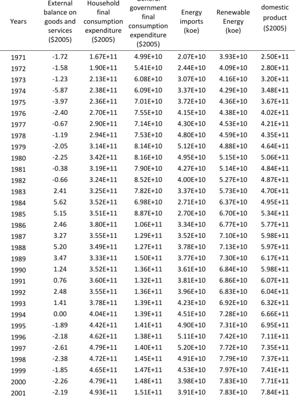
The raw data to perform the model correspond to the official available data based on Brazil, provided by the Word Bank and the Brazilian Energy Research Company.
The simulation period extends from 1971 to 2030. The period of 1971-2012 (which corresponds to 31 years) was used to fix the parameters of the model and 2013-2030 (18 years) corresponds to the forecast period, under the assumption of different scenarios concerning the evolution of the income, the evolution of the energy mix, and the efficiency of the used technology.
21
Services, residential and transportation sector. While the index j runs over seven type of fuels, which are (1) natural gas, (2) liquefied petroleum gases, (3) motor gasoline, (4) gas/diesel oil, (5) fuel oil, (6) petroleum coke and (7) renewable, alternative and nuclear energy.
3.2 Economic submodel
This methodology presents a key point the explicit inclusion of the effect of renewable energy on the GDP, allowing to establish a link between economic indicators and CO2 emissions. Also this method considers that renewable energy can
increase GDP through substitution of the energy import which has direct and indirect effects on increasing GDP and trade balance (Chien and Hu, 2008). The expenditure approach to form the GDP is
𝑄 = 𝐶𝑎 + 𝐼 + 𝐺 + 𝑇𝐵 (4)
Where:
Ca - is the final household consumption expenditure I - is the gross domestic capital formation
G - is the general government final consumption expenditure TB - is the trade balance
However, there is a particular concern which it is important to highlight, the variable G should be removed of the model estimation in order to avoid multicollinearity. The system of the theoretical GDP formation model is composed of the equation below
𝑄 = 𝑎1. 𝐼 + 𝑎2. 𝑇𝐵 + 𝑎3. 𝐶𝑎 + 𝑎4. 𝐸𝑖𝑚𝑝+ 𝑎5. 𝑅𝑁 + ∊1 (5)
Where:
𝐸𝑖𝑚𝑝 - is the energy import
∊ - are residuals
𝑎1…𝑎5 - are the coefficients
The data used to calibrate the model corresponds to the period of 1971-2012 and was extracted from the official dataset of the country. In equation 5 the GDP is positively influenced by consumption (𝑎3 = +7.882 10- 1), energy import (𝑎4= +1.728
10-2 $2005/koe) and renewable energies (𝑎5 = +6.698 10 $2005/koe), however, capital
formation (𝑎1= -5.309 10-1) and trade balance (𝑎2= -4.253 10-1) had a negatively
influenced.
3.3 Energy consumption and productive sectoral structure submodel
Energy consumption refers to the use of primary energy before transformation into any other end-use energy, which is equal to the local production of energy plus imports and stock changes, minus the exports and the amount of fuel supplied to ships and aircrafts engaged in international transport. Energy intensity is defined as the ratio of energy consumption and GDP.
3.4 CO2 intensity and energy matrix submodel
CO2 intensity of a given country corresponds to the ratio of CO2 emissions and
the total consumed energy written in terms of mass of oil equivalent.
𝐶𝑂2𝑖𝑛𝑡 =∑∑𝑖𝑗𝐶𝑖𝑗
𝑖𝑗𝐸𝑖𝑗 (6)
The value of the CO2int in a given year depend on the particular energy mix
during that year. Mij gives the energy matrix, but is more convenient to sum over the
different sectors and aggregate the fossil fuel contributions, therefore, it was defined for each type of fuel (j=1 to 7).
𝑀𝑗 = ∑𝑖𝐸𝑖𝑗
23
Hence, the share of expended fossil energy is given by 6∑i=1= Mj , while M7
is the share of used renewable energy in the country. It was assumed that M7 does not
contribute to the CO2 emissions.
The emission factors, Uij, were taken from the IPCC Guidelines for National Greenhouse Gas Inventories (2006) to estimate C02 emission of each fuel. The used
values are highlighted in gray (Table 2). According to IPCC combustion processes are optimized to derive the maximum amount of energy per unit of fuel consumed, hence delivering the maximum amount of CO2. Efficient fuel combustion ensures oxidation of
the maximum amount of carbon available in the fuel. CO2 emission factors for fuel
combustion are therefore relatively insensitive to the combustion process itself and hence are primarily dependent only on the carbon content of the fuel.
Table 2. Default CO2 emission factors for combustion.
DEFAULT CO2 EMISSION FACTORS FOR COMBUSTION 1
Fuel type English description
Effective CO2 emission factor (kg/TJ) 2
Other Petroleum Products 20.0 1 73 300 72 200 74 400
1 The lower and upper limits of the 95 percent confidence intervals, assuming lognormal distributions,
fitted to a dataset, based on national inventory reports, IEA data and available national data. A more detailed description is given in section 1.5
2 TJ = 1000GJ 3
The emission factor values for BFG includes carbon dioxide originally contained in this gas as well as that formed due to combustion of this gas.
4 The emission factor values for OSF includes carbon dioxide originally contained in this gas as well as
that formed due to combustion of this gas
5
Includes the biomass-derived CO2 emitted from the black liquor combustion unit and the
biomass-derived CO2 emitted from the kraft mill lime kiln.
25
3.5 Model equations and causal diagram
In the equation presents along this chapter it is possible to see how the model is split in two different parts: energy and productive sectoral submodels, equations (2) and (3) , and economic submodel, equation 5.
In the first case, the energy and, in particular, the amount of renewable energy, Ej=7, are calculated. In the second one, the value of GDP is calculated in terms of its
components, one of which is renewable energy. These two parts are coupled throught the renewable energy terms which generates a feedback mechanism positive in the case of Brazil.
Figure 2 presents the schematic view of the model. Where the feedback mechanism is highlighted. This way of presenting the model is extremely useful because it allows us to see the driving forces of CO2 emissions in a hierarchical way,
showing the causality relationship between the different variables. It can be observed that the CO2 emitted into the atmosphere has several connections with the variables
of the model: economic growth, productive sectoral structure, energy consumption, and energy matrix.
A more quantitative way of presenting how the different variables are extrapolated is through the difference equations that should be solved:
𝑄(𝑡) = 𝑎1𝐼(𝑡) + 𝑎2𝑇𝐵(𝑡) + 𝑎3𝐶𝑎(𝑡) + 𝑎4𝐸𝑖𝑚𝑝(𝑡) + 𝑎5𝑅𝑁(𝑡 − 1) (8)
𝐸𝑗(𝑡) = ∑ 𝑆𝑖(𝑡). 𝐸𝐼𝑖 (𝑡). 𝑀𝑖𝑗(𝑡). 𝐺𝐷𝑃(𝑡)𝑖 (9)
𝑅𝑁(𝑡) = 𝐸7(𝑡) (10)
𝑦(𝑡) = 𝑦(𝑡 − 1). (1 + 𝑟𝑦) (11)
Where Si(t), EI(t), Mij (t), I(t), TB(t), Ca (t) and Eimp(t) evolve following Eq. (11)
while the parameters ai have constant values. Note that index j runs over the type of
energy sources, while i on the industrial sectors; j=7 corresponds to renewable and alternative energy. t=o corresponds to the reference year 2012 and t is given in number of years since 2012. The value of ry is fixed through the definition of the used
scenario. In the case of the BS scenario one should use a value of ry that depends on
the time. In this case ry roughly corresponds to the yearly average increase over the
period 1971-2012.
3.6 Model validation and verification
27
𝑀𝐴𝑃𝐸(%) =𝑁1 ∑ |𝐷𝑎𝑡𝑎𝑖−𝑀𝑜𝑑𝑒𝑙 𝑖
𝐷𝑎𝑡𝑎𝑖 | 𝑁
𝑖=1 𝑥 100 (12)
Where:
N - Number of data Datai - is the real data
4. RESULTS AND DISCUSSION
4.1 Brazil in numbers
4.1.1 Overview
Brazil is the fifth largest country in the world in terms of area and population, occupying approximately half of the entire South America. Brazil extends through 8,515,692 km² divided into 99.3 % of land and 0.7% of water. The coastline stretches for 7,491 km (Brazilian Institute of Geography and Statistics-BIGS, 2016).
First country to sign the Convention on Biological Diversity, Brazil is the most biologically diverse nation in the world with six terrestrial biomes and three large marine ecosystems, and with at least 103,870 animal species and 43,020 plant species currently known in Brazil. There are two biodiversity hotspots currently acknowledged in Brazil – the Atlantic Forest and the Cerrado, and 6 biosphere reserves are globally recognized by the United Nations Educational, Scientific and Cultural Organization (UNESCO) in the country (ME, 2011). This diversity makes Brazil one of the 17 mega-diverse countries in the world (United Nations Environment Programme-UNEP, 2002).
Brazil’s Human Development Index (HDI) was 0.755 in 2014 (UN Development Program, 2015), placing it in 75th position of 188 countries and territories. Between 1980 and 2014, Brazil’s HDI soared from 0.547 to 0.755, an increase of 38.1% which represents an annual growth of 0.95%.
29
Table 3. Brazilian total population from 2000 to 2060.
Years Population Years Population Years Population
2000 173,448,346 2020 212,077,375 2040 228,153,204
2001 175,885,229 2021 213,440,458 2041 228,287,681
2002 178,276,128 2022 214,747,509 2042 228,359,924
2003 180,619,108 2023 215,998,724 2043 228,343,224
2004 182,911,487 2024 217,193,093 2044 228,264,820
2005 185,150,806 2025 218,330,014 2045 228,116,279
2006 187,335,137 2026 219,408,552 2046 227,898,165
2007 189,462,755 2027 220,428,030 2047 227,611,124
2008 191,532,439 2028 221,388185 2048 227,256,259
2009 193,543,969 2029 222,288,169 2049 226,834,687
2010 195,497,797 2030 223,126,917 2050 226,347,688
2011 197,397,018 2031 223,904,308 2051 225,796,508
2012 199,242,462 2032 224,626,629 2052 225,182,233
2013 201,032,714 2033 225,291,340 2053 224,506,312
2014 202,768,562 2034 225,896,169 2054 223,770,235
2015 204,450,649 2035 226,438,916 2055 222,975,532
2016 206,081,432 2036 226,917,266 2056 222,123,791
2017 207,660,929 2037 227,329,138 2057 221,216,414
2018 209,186,802 2038 227,673,003 2058 220,254,812
2019 210,659,013 2039 227,947,957 2059 219,240,240
2060 218,173,888
Source: BIGS, 2013.
4.1.2. Economy
According to the World Bank (2016), in 2015 Brazil was the ninth largest economy in the world, with a GDP 1,774,725 USD (2011 purchasing power parity-PPP). Moreover, the GDP per capita in 2015 was 8,538 USD (2011 PPP).
In addition, the World Bank (2016) affirms that Brazil's economic and social progress between 2003 and 2014 took 29 million people away from poverty, as well as the social inequality dropped significantly. The income level of 40% of the poorest population rose, at the average of 7.1% (in real terms) between 2003 and 2014, compared to a 4.4% income growth for the population as a whole. However, the rate of poverty and inequality reduction has been showing signs of stagnation since 2015.
2014. The GDP contracted by 3.8% in 2015. The realignment of regulated prices combined with the pass-through of exchange rate depreciation caused an inflation peak in 2015 (with 12-month accumulated inflation rate of 10.7% in December of 2015), exceeding the upper limit of the target band (6.5%).
The economic crisis - coupled with the ethical-political crisis faced by the country - has contributed to those numbers. On August 31st, with public opinions divided, the Resolution N°35 of 2016 was published in the Official Newspaper of the Union, which established the impeachment of Mrs. Dilma Vana Rousseff, who had been the democratically elected President of the Brazilian Republic (FRB,2016).
The fiscal adjustment is undermined by budget rigidities and by a difficult political environment. Less than 15% of expenditures in Brazil are expected to be discretionary. Most public spending is mandatory (mandated by the Constitution or other legislation) and increases in line with revenues, nominal GDP growth, or other pre-established rules. Additionally, a large portion of revenues for education and health care are earmarked. Attempts to pass legislation to increase revenue collection in the short term and address issues of a more structural nature - such as pensions - have so far fallen short of the government's intentions (Word Bank, 2015).
4.1.3 Energy analysis
The information summarized below was obtained from the 2015 Brazilian Energy Balance report published by the Brazilian Ministry of Mines and elaborated by the Energy Research Company (BERC, 2015).
31
the electricity network. Net imports of 33.8 TWh, added to internal generation, allowed a domestic electricity supply of 624.3 TWh and the final consumption was 531.1 TWh.
Figure 3 illustrates the structure of the domestic supply of electricity in Brazil in 2014. It can be observed that Brazil presents an electricity matrix predominantly renewable, and the domestic hydraulic generation accounts for 65.2% of the supply. Adding imports, which are also mainly from renewable sources, it can be stated that 74.6% of electricity in Brazil comes from renewable sources.
Figure 3. Domestic electricity supply by source. Source:BERC, 2015.
On the consumption side, the residential sector grew by 5.7%. The industrial sector recorded a decrease of 2.0% in electricity consumption over the previous year (2013). The other sectors - public, agriculture and livestock, commercial and transportation - when analyzed collectively showed a positive growth of 7.0% over 2013. The energy sector increased 4.8%. Figure 4 shows the domestic electricity supply by sector.
Finally, wind and solar farms were responsible for 37.6% of the remaining growth in the national grid installed capacity.
Figure 4. Domestic electricity supply by sector. Source: BERC, 2015.
Petroleum and Oil Products: The domestic production of oil in 2014 reached an average of 2.25 million barrels per day, of which 93% are offshore. In addition, the shale oil production reached 0.3 million m³. The production of oil products in domestic refineries amounted to 110.4 million toe, highlight for diesel and gasoline, which accounted for 39% and 20%, respectively, of the total.
Natural Gas: The average daily production for the year was 87.4 million m³/day and the volume of imported natural gas was an average of 52.9 million m³/day. Thus, the natural gas share in the national energy matrix reached the level of 13.5%. The thermal power generation with natural gas (including self-producer and public service power plants) increased by 17.5% reaching a level of 81.1 TWh. In 2014 the average consumption in the electricity sector reached 51.7 million m³/day. It represents an increase of 20.9% compared to 2013. The share of natural gas intended for transformation centers overcomes the sector consumption reaching 51% of the total, which 8% is intended for oil items production and 43% for electricity generation.
Steam and Metallurgical Coal: National steam coal, produced in the southern states of Brazil, is used for electric generation. The demand of steam coal for this final
33
use increased 9.4% in 2014 when compared to the previous year. In 2014, the steel industry showed a 7.5% increase in consumption of metallurgical coal due to the increase of crude steel production via reducing coke in this period (2.1%).
Wind Energy: The production of electricity from wind power reached 12,210 GWh in 2014. This represents an 85.6% increase over the previous year, when it had reached 6,578 GWh. In 2014, the installed capacity for wind generation in the country increased by 122%. According to the Power Generation Database from National Agency of Electric Energy (NAEE), the national wind farm grew 2.686 MW, reaching 4,888 MW by the end of 2014.
Biodiesel: In 2014 the amount of biodiesel produced in Brazil reached 3,419,838 m³, against 2,917,488 m³ in the previous year. Thus, there was an increase of 17.2% in available biodiesel in the national market. The percentage of biodiesel compulsorily added to mineral diesel was increased to 6% in July and 7% in November 2014. The main raw material was the soybean oil (69.2%), followed by tallow (17%).
Sugarcane, Sugar and Ethanol: According to the Ministry of Agriculture, Livestock and Food Supply, the sugar cane production in the calendar year 2014 was 631.8 million tons. This amount was 2.5% lower than in the previous calendar year, when the milling was 648.1 million tons. In 2014 the national sugar production was 35.4 million tons, 5% lower than the previous year, while the production of ethanol increased by 3.3%, yielding the amount of 28,526 m³. About 57.1% of this total refers to hydrous ethanol: 16,296 m³. In comparative terms, the production of this fuel increased by 4.4% compared to 2013. Regarding the production of anhydrous ethanol, which is blended with gasoline A to form gasoline C, there was an increase of 1.9%, totaling 12,230 m³. The Total Recoverable Sugar (ATR) in sugarcane, which is the amount of sugar available in raw material minus the losses in the manufacturing process, kept stable and recorded averages of 136.3 and 132.6 ATR/ton of cane for the 2012-2013 and 2013-2014 harvests, respectively.
Table 4. Domestic energy supply from 2005 to 2014
Sources (%) 2005 2006 2007 2008 2009 2010 2011 2012 2013 2014 Non-renewable energy 55.9 55.4 54.5 54.4 53.2 55.3 56.5 58.2 59.6 60.6
Petroleum and oil products 38.8 37.9 37.5 36.7 37.9 37.8 38.6 39.3 39.3 39.4 Natural gas 9.4 9.6 9.3 10.3 8.8 10.2 10.2 11.5 12.8 13.5 Coal and coke 6.0 5.7 5.7 5.5 4.6 5.4 5.7 5.4 5.6 5.7 Uranium 1.2 1.6 1.4 1.5 1.4 1.4 1.5 1.5 1.4 1.3 Other none-renewable 1.0 1.0 1.0 0.0 1.0 0.0 0.0 0.0 1.0 1.0
Renewable energy 44.1 44.6 45.5 45.6 46.8 44.7 43.5 41.8 40.4 39.4
Hydraulic 14.9 14.9 14.9 14.1 15.2 14.0 14.7 13.8 12.5 11.5 Firewood and charcoal 13.1 12.7 12.0 11.6 10.1 9.7 9.6 9.1 8.3 8.1 Sugar cane products 13.8 14.6 15.9 17.0 18.1 17.5 15.7 15.4 16.1 15.7 Other renewable source 2.3 2.5 2.7 2.9 3.4 3.5 3.5 3.5 3.6 4.1
Source: BERC, 2015.
Figure 5. Domestic energy supply in 2014. Source: BERC, 2015.
4.1.4 Forecasts for 2030
The Brazilian National Energy Plan 2030 (BERC, 2007) establishes different economic and energy demand scenarios considering four different GDP trajectories, the scenarios have been based on different annual GDP growth rates for the period between 2005 and 2030, as follows: Scenario A 5.1%, B1 scenario 4.1%, B2 scenario
39%
16% 14%
11% 8%
6% 4% 1% 0.6%
Petroleum and oil products Sugar cane products Natural gas Hydraulic Firewood and charchoal Coal and coke
35
3.2% and scenario C 2.2%. The plan, however, prioritizes the scenario B1 and Figure 6 shows the evolution of the domestic energy supply structure.
The evolution of the energy matrix in the period 2005-2030 shows an expansion in its diversification. Thus, within this period, it is expected a significant reduction from 13% to 5.5% in the use of wood and charcoal; an increased share of natural gas from 9.4% to 15.5%; a reduction of oil and derivatives share from 38.7% to 28%; an increase in the share of derived products from sugarcane and other renewables (ethanol, biodiesel and others) from 16.7% to 27.6%.
Figure 6. Evolution of the domestic energy supply structure Source: MME, 2007.
to GDP, this domestic energy supply would imply 5% reduction in energy intensity. The value expressed in toe/ (US$ 1,000) is 0.275 in 2005 and 0.261 in 2030.
The import of energy focuses on coal for steel, natural gas and electricity, the latter coming mainly from the Paraguayan side of Itaipu. It can be stated that, according to the same assumptions, Brazil would find a situation in this period 2005-2030, which was close to energy self-sufficiency.
4.1.5. Brazil and the United Nations Framework Convention on Climate Change
Despite the fact that Brazil was responsible for only 1.45% of global emissions in 2013 (Word Bank, 2016), in September 2015, the Brazilian Government communicated to the Secretariat of the United Nations Framework Convention on Climate Change (UNFCCC) their intended Nationally Determined Contribution (iNDC) to the new agreement under the Convention that was adopted at the 21st Conference of the Parties (COP-21) to the UNFCCC in Paris (FRB, 2015).
In this document, the Brazilian contribution intends to be committed to reduce greenhouse gas emissions by 37% below 2005 levels (reference point) by 2025. In addition, Brazil proposed, for reference purpose only, a subsequent indicative contribution, which was to reduce greenhouse gas emissions by 43% below 2005 levels by 2030. These goals cover 100% of the territory, the Brazilian economy, and include CO2, CH4, N2O, perfluorocarbons, hydrofluorocarbons and SF6 emissions.
Brazil hopes to achieve these cuts by implementing measures that are in line with a transition to a low-carbon economy, mainly:
increasing the share of sustainable biofuels in the Brazilian energy mix to approximately 18% by 2030, by expanding biofuel consumption, by increasing ethanol supply, by increasing the share of advanced biofuels (second generation), and also by increasing the share of biodiesel in the diesel mix;
37
in the Brazilian Amazonia, zero illegal deforestation by 2030 and compensating for greenhouse gas emissions from legal suppression of vegetation by 2030; and restoring and reforesting 12 million hectares of forests by 2030, for multiple purposes; finally, enhancing sustainable native forest management systems, through georeferencing and tracking systems applicable to native forest management, with a view to curbing illegal and unsustainable practices;
in the energy sector: by achieving 45% of renewables in the energy mix by 2030. Including: the expanding the use of renewable energy sources other than hydropower in the total energy mix to between 28% and 33% by 2030; the expanding the use of non-fossil fuel energy sources domestically, increasing the share of renewables (other than hydropower) in the power supply to at least 23% by 2030, by raising the share of wind, biomass and solar; and, achieving 10% efficiency gains in the electricity sector by 2030.
Furthermore, Brazil also intends to:
in the agriculture sector: strengthen the Low Carbon Emission Agriculture Program as the main strategy for sustainable agriculture development. This includes: restoring an additional 15 million hectares of degraded pasturelands by 2030 and enhancing 5 million hectares of integrated cropland-livestock-forestry systems (ICLFS) by 2030;
in the industry sector: promote new standards of clean technology and further enhance energy efficiency measures and low carbon infrastructure;
in the transportation sector: promote efficiency measures and improve infrastructure for transport and public transportation in urban areas.
4.1.6. Data
According to the previously information presented about Brazil, this subchapter shows in table format all the compiled data, which was necessary to fill up the model.
39
Table 6. Brazilian general data. Part II.
2000 187441584000 109151103000 327983814000 2001 190711767000 112423995000 337433673000 2002 195758711000 111883929000 332266870000 2003 198976524000 108723416000 321621569000 2004 210041760000 114889113000 337826042000 2005 215331854000 116822529000 347308904000 2006 222817428000 119035502000 347668270000 2007 235459748000 123994607000 363212683000 2008 248579623000 130676967000 387675240000 2009 240453393000 123396972000 367147374000 2010 265862911000 142197735000 419754156000 2011 270026935000 147344496000 439412943000 2012 281724649000 159305890000 470029000000
Table 7. Information about Brazilian agriculture sector.
Years E1 (toe)
QiS1
41
1997 7528143 29773497162 0.252847133 1998 7308493 30881986380 0.236658778 1999 7536184 32967958777 0.228591154 2000 7322063 33765662219 0.216849368 2001 7728679 35958389316 0.214933961 2002 7809259 38477327408 0.202957417 2003 8149978 40723243107 0.200130868 2004 8274035 41659945213 0.198608879 2005 8357612 38958191676 0.214527723 2006 8550542 40817363327 0.20948295 2007 9054700 42167678540 0.214730806 2008 9908631 44514949276 0.22259109 2009 9551669 42877973582 0.222764005 2010 10026747 45772592734 0.219055697 2011 9998667 48351978361 0.206789203 2012 10361298 47208027453 0.219481702
Table 8. Information about Brazilian manufacturing sector.
1994 48714651 158800000000 0.306673849 1995 49836986 169400000000 0.294229327 1996 51777402 171900000000 0.301161269 1997 54020557 176100000000 0.30675709 1998 55451871 166400000000 0.333270908 1999 57394330 160800000000 0.356888827 2000 58425520 155300000000 0.376267513 2001 58798037 153800000000 0.382307459 2002 62519161 157500000000 0.397042378 2003 65284855 158400000000 0.412273752 2004 68958858 172200000000 0.400554261 2005 70041303 158800000000 0.441056515 2006 73155403 160400000000 0.456010775 2007 77938001 171400000000 0.454696143 2008 78371741 178900000000 0.438120444 2009 73934426 167800000000 0.440511751 2010 82384369 186400000000 0.441974475 2011 85380217 194400000000 0.439118129 2012 85457509 194300000000 0.439797946
Table 9. Information about Brazilian energetic sector.
43
1991 13810942 25857000000 0.534135866 1992 13699348 26702000000 0.513051329 1993 13857328 28491000000 0.486380046 1994 14855638 28671000000 0.518133036 1995 14342093 27392000000 0.523596349 1996 15443295 25116000000 0.614881676 1997 17063396 25892000000 0.659024426 1998 16107878 26411000000 0.609899361 1999 15346391 28792000000 0.533002513 2000 15067330 44530000000 0.338366005 2001 15742729 45588000000 0.345327611 2002 16645791 46882000000 0.355057098 2003 18235151 48657000000 0.374767723 2004 18945485 51151000000 0.370386043 2005 20417013 59446000000 0.343456124 2006 21684932 62106000000 0.349157688 2007 24244030 64631000000 0.375113316 2008 27877201 66467000000 0.419416311 2009 26170480 65993000000 0.396564398 2010 27440718 71629000000 0.383096402 2011 25506337 74156000000 0.343956441 2012 26107941 74951000000 0.348335075
Table 10. Information about Brazilian tertiary sector.
1988 60098346 399700000000 0.150344842 1989 62043994 413400000000 0.150079664 1990 61448787 409700000000 0.149973753 1991 63538728 417300000000 0.152259497 1992 63933204 420200000000 0.152163931 1993 65077987 433400000000 0.1501708 1994 67884840 451100000000 0.150491418 1995 72385412 469700000000 0.154115583 1996 76821906 483900000000 0.158757251 1997 79751378 502800000000 0.158608825 1998 82736622 513400000000 0.161156963 1999 82824877 517900000000 0.159909155 2000 82103480 537400000000 0.152775902 2001 81195599 548400000000 0.148053516 2002 84303846 564900000000 0.149243988 2003 83196304 569200000000 0.146171058 2004 87952728 599000000000 0.146833539 2005 90412680 634400000000 0.14251177 2006 91197620 663600000000 0.137429742 2007 98393767 705000000000 0.13956089 2008 106391617 743400000000 0.143105335 2009 107945393 755300000000 0.142917061 2010 115681669 805900000000 0.1435425 2011 118872472 836200000000 0.14216534 2012 124143966 858700000000 0.144569048
Table 11. Energy by type of fuels in agriculture sector.
45
Table 12. Energy by type of fuels in imanufacturing sector.
1981 335.15 952.58 155.80 382.77 8979.53 3958.99 18302.49
Table 13. Energy by type of fuels in energetic sector.
47
Table 14. Energy by type of fuels in tertiary sector.
Years ktoe
49
4.2 Estimates
4.2.1 MAPE
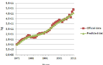
MAPE values for the main variables of the model are show in the Table 15, and Figures 7, 8, 9, 10 and 11. The main difference between official data and the predicted one due to the application of Hodrick-Prescott filter (1997).
Table 15. MAPE values for the main variables of the model.
Variable MAPE (%)
GDP 2.4%
Efossil 6.8%
RN 2.8%
Etotal 2.4%
CO2 4.4%
Figure 8. Fossil energy official and predicted data.
Figure 9. Renewable energy official and predicted data.
51
Figure 11.CO2 emissions official and predicted data.
4.2.2 Scenarios
In this research we calculate the value of CO2 emissions in the medium term. As
it was said before, CO2 emissions depend on several variables, therefore we have
defined four scenarios concerning the growth of GDP, the evolution of the energy matrix, of the productive sectoral structure, and the improvement of energy efficiency for the period 2013-2030.
1.Baseline scenario (BS): GDP, energy matrix and productive sectoral structure will evolve through the smooth trend of the period 1971-2012, extrapolated to 2013-2030 using the geometric growth rate method.
2. Doubling of the GDP (SC-2 scenario): GDP in 2030 will be more than double that of 2012. To generate this scenario a constant annual growth of the GDP formation components (I, TB, C, Eimp) of 4.1% per year between 2012 and 2030 is assumed. This
3. Doubling of the GDP and changed the energetic matrix (SC-3 scenario): The doubling of the GDP and the change of the productive sectoral structure as in the SC-2 scenario are considered, however, the consumption of renewable and nuclear fuel will increase 9% while the natural gas growth 2%. At the same time the consumption of oil and its derivatives will decrease 10% in the whole period.
4. 3. Doubling of the GDP, changed the energetic matrix and improved the
efficiency of energy use (SC-4 scenario): The doubling of the GDP, the change of the productive sectoral structure and the reordering of fuel use are the same as in the SC-3 scenario. Moreover an improvement in the efficiency of energy use is implemented with a reduction in the sectoral energy intensity of 5% in the whole period.
4.2.3 Economic estimates
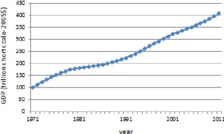
The estimate values of GDP for the pre-established scenarios are presented in Figure 12, Figure 13 and Appendix 1. The first projection refers to 2013 and for the BS scenario corresponds nearly to 1,2 trillion short scale 2005$*. For the year 2030, the BS scenario reaches 2,5 trillion short scale 2005$, which corresponds to more than double that of 2013.
53
Figure 12. GDP of Brazil for the period 1971-2011.
Figure 13. GDP of Brazil for the period 2010-2030.
4.2.4 Energy estimates
4.2.4.1 Total energy
Figure 14, Figure 15 and Appendix 2 illustrate the progress of the total energy consumption. In 2013 the projections demonstrated 277130556 toe; 279586116 toe; 279586116 toe; and 278778771 toe for BS scenario, SC-2, SC-3 and SC-4, respectively. However, for 2030, the numbers are superior, being 550593722 toe; 829104077 toe; 774498261 toe; and, 629445279 toe for the same order above.
Further, in 2030 the total energy consumption of the SC-2 corresponds to 50.6% higher than the BS scenario. Likewise, the SC-3 is 40.6% higher than BS scenario. These two last scenarios show the growth of the energy consumption due to the increase of GDP and to the changes of the productive sectoral structure. Lastly, SC-4 generates a consumption of only 14.3% higher than the BS scenario. It distinctly reveals the benefits of the reduction of energy intensity.
55
Figure 15. Total energy consumption of Brazil for the period 2010-2030.
The previsions of the consumption of fossil energy (Figure 16 and Appendix 3) in 2030 in the BS scenario is 306448946 toe, while in SC-2 is 444402429 toe (45% higher than the BS scenario), in SC-3 is 371067222 toe (21% higher than the BS scenario) and in SC-4 is 305332983 toe (0.66% lower than the BS scenario). Moreover, the estimations of the consumption of renewable energy are elucidated in Figure 17 and Appendix 4. As we can see, in 2030 the results correspond nearly to 290212188 toe, 443429030 toe, 405460499 toe and 325638742 toe in the BS, SC-2, SC-3 and SC-4 scenarios, representing increases about of 53%, 40% and 12% compared to the BS scenario, respectively.
Figure 17. Renewable energy consumption of Brazil for the period 1971-2030.
4.2.4.2 Energy by sector
The change in the behavioral pattern of energy consumption in the primary sector can be seen in Figure 18 and 19, the first makes reference to BS scenario and SC-2, while the second refers to the SC-3 and SC-4.
57
Figure 19. Energy consumption of Brazilian primary sector for the SC-3 and SC-4 scenarios during the period 2000-2030.
In the BS scenario and SC-2, for the next years the fuel oil tends to have an insignificant consumption, while gas/diesel oil will decline 10% and renewable, alternative and nuclear energy will rise 12% (Appendix 5). For the same period, in 2030, the SC-3 and SC-4 shows the same disappearance of fuel oil in the agricultural sector, but the reduction in gas/diesel oil will be 5% and the accretion in the renewable, alternative and nuclear energy will be 7% (Appendix 6).
In the manufacturing sector, the BS scenario and SC-2 result in a nearly rise from 6 to 16% of natural gas and from 58 to 63% of renewable, alternative and nuclear energy. At the same time, the liquefied petroleum gases, gas/diesel oil, fuel oil and petroleum coke practically keep the same values (Figure 20 and Appendix 7).
Figure 20. Energy consumption of Brazilian manufacturing sector for the BS and SC-2 scenarios during the period 2000-2030.
Figure 21. Energy consumption of Brazilian manufacturing sector for the SC-3 and SC-4 scenarios during the period 2000-2030.
59
21% of natural gas, up 4.5% of gas/diesel oil and up 56% of renewable, alternative and nuclear energy (Figure 23 and Appendix 10).
Figure 22. Energy consumption of Brazilian energetic sector for the BS and SC-2 scenarios during the period 2000-2030.
Finally, the tertiary sector presents a reduction on liquefied petroleum gases from 8.2 to 2.7%, and gas/diesel oil from 29.5 to 24.3%. At the same time, the increase on natural gas is only 1%, the motor gasoline growth up to 26% and the renewable, alternative and nuclear energy up to 44.7%, as it is possible to see in Figure 24 and Appendix 11.
Figure 24. Energy consumption of Brazilian tertiary sector for the BS and SC-2 scenarios during the period 2000-2030.