Review on detection/analysis ventricular late potentials

Texto completo

(1)ISBN: 959-250-061-4. Review on Detection/Analysis of Review on Detection/Analysis of Ventricular Late Ventricular Late Potentials Potentials. Autor: Alberto Taboada Crispi Autor: Alberto Taboada Crispi.

(2) © Alberto Taboada, 2003 © Editorial Feijóo, 2003. Diseño y cubierta: Roberto Suárez. Editorial Feijóo Carretera a Camajuaní Km 5 ½ Santa Clara, Villa Clara C. P.: 54830.

(3) INDEX Chapter 1. Introduction/ 3 1.1. Cardiovascular disease and sudden cardiac death/ 3 1.1.1. SCD: the treatments/ 4 1.1.2. Need of stratification techniques/ 4 1.2. Non-invasive versus invasive diagnostic techniques/ 5 1.2.1. Invasive technique: Electrophysiological Studies/ 5 1.2.2. Non-invasive techniques/ 6 1.2.3. Indexes of affectiveness/ 8 1.2.4. SCD: model and combination of techniques/ 10 1.3. Ventricular Late Potentials (VLPs)/ 10 1.3.1. Origin of VLPs/ 10 1.3.2. VLPs and cardiac care/ 13 1.3.3. Characteristics of VLPs. Why are they so difficult to detect?/ 15 Chapter 2. Current clinical and research approaches/ 20 2.1. Introduction/ 20 2.2. Instrumentation requirements/ 20 2.3. Signal enhacement techniques/ 26 2.3.1. Introduction/ 26 2.3.2. Coherent averaging/ 28 2.3.3. Optimalfiltering and weighting averaging/ 31 2.3.4. Adaptive filtering/ 32 2.3.5. High-Order Spectrum/ 34 2.3.6. Denoising with Wavelets/ 34 2.4. Detection/analysis/ 35 2.4.1. Time domain/ 35 2.4.2. Frequency domain/ 38 2.5. Summary/ 43 References/ 44.

(4) Chapter 1 - Introduction Cardiovascular disease (CVD) is the leading cause of death worldwide and sudden cardiac death (SCD) is responsible for 50%. Patients at risk for SCD have several treatments available to them. However, an accurate and non-invasive method to identify those at risk has been missing. Ventricular late potentials (VLPs) appear associated with ventricular tachycardia (VT) preceding most instances of SCD. Detection of VLPs has proved to have potential as a VT predictor, as well as a diagnostic marker for several cardiac abnormalities [33] [26] [47].. 1.1 Cardiovascular disease and sudden cardiac death CVD is a major cause of death all over the world. The incidence rates are sex- and agedependent and can change from one country to another, but they are always impressive. To mention some examples published in [95], around 1995, mortality rates for CVD in men was 232.7 deaths per 100 000 population in Japan, the lowest reported, and as high as 1 051.7 per 100 000 in the Russian Federation. In Canada, 36% of all deaths are due to CVD. Of these, nearly 56% are from ischemic heart disease (IHD). More specifically, of the deaths due to IHD, 50% can be attributed to myocardial infarction (MI) [95]. Major risk factors for CVD are well known, but no significant improvements have been reached to keep them under control. The epidemic of CVD will continue in the years to come, due to the high prevalence of smoking, physical inactivity, high blood pressure, dyslipidemias, obesity and diabetes all around the world. To make things worse, the number of persons suffering from CVD is expected to grow because of the increasing numbers of the elderly population, which is the most likely to develop cardiovascular problems. SCD is the term given to natural death from cardiac causes, with an abrupt loss of consciousness preceding the acute symptoms, in a person with or without diagnosed cardiopathy [105]. Most SCDs are thought to be initiated by VT and/or ventricular fibrillation (VF), two of the most serious types of cardiac arrhythmia [155]. These lethal arrhythmias affect the main pumping chambers of the heart, the ventricles. In VT, the ventricles beat too fast, compromising their ability to pump blood. VTs consist of 3 or more consecutive ventricular depolarisations at rates of 100 beats per minute or higher; they can be classified as non-sustained ventricular tachycardias (nsVT), when they disappear spontaneously in less than 30 seconds, or sustained ventricular tachycardias (sVT), when last longer. In VF, the ventricles contract in a disorganised fashion that results in total loss of their blood-pumping action. VF, unless interrupted by an electrical shock (defibrillation), is fatal and is the immediate cause of SCD in the majority of cases. It is important to note that VT may progress into VF.. 3.

(5) Half of the deaths due to CVD can be classified as SCD, that is, around 10% to 15% of all natural deaths. In the United States alone, SCD affects around 500 000 people each year, almost 2 cases per 1 000 inhabitants and claims the lives of about 70% of them [105] [17]. These figures, although generated from calculations and likely to be inaccurate, have gone unchanged for 20 years. 1.1.1 SCD treatments Most people who suffer SCD can be saved if they are resuscitated promptly. Different treatments have been used to handle VT and SCD, among them, antiarrhythmic drug therapy to prevent and control arrhythmias, surgical procedures (catheter ablation) to destroy arrhythmic substrate [96] and implantation of antitachycardiac devices like the implantable cardioverter-defibrillator (ICD). The latter is a device that detects when the heart goes into VT or VF and ends the arrhythmia by applying electrical shocks to the heart [172]. In recent years, treatments have been improved and many studies have tried to find the best choice [105] [172] [74] [156]. Until now, there has been controversy as to whether pharmacotherapy can work as well as the ICD [172] [156]. In 1997, a large clinical study, the Amiodarone versus Implantable Defibrillator trial (AVID) [15], had to be stopped prematurely because it showed that patients who received ICD devices had a much lower mortality than those treated with amiodarone or sotalol (another antiarrhythmic drug). For those patients who cannot receive an ICD, amiodarone is an excellent treatment option; however, based on available data, AVID and some other extensive trials like the Multi-centre Automatic Defibrillator Implantation Trial (MADIT) and the Multicentre UnSustained Tachycardia Trial (MUSTT ) [154] [108] agree that the ICD device is the most effective treatment. At present, some more detailed trials are progressing toward completion [154]. One of which, the Sudden Cardiac Death Heart Failure Trial (SCD-HeFT), is due to report in 2003 [108]. ICD therapy is expensive. Therapies in medicine are generally considered “costeffective” if they cost less than $50 000 per year life saved [136] [48]. The preliminary figures for ICD plus doctor and hospital fees associated with the implantation and subsequent monitoring of the device can be in the range of $60 000 to $70 000 [17] and around $34 000 for drug therapy. On the other hand, antiarrhythmic drug therapy can have some unexpected side effects, like congestive heart failure and an increased risk of SCD, so it should be used with caution. Hence, identification of those patients at higher risk is imperative. From a clinical point of view, the challenge is to find who is really at risk of SCD and needs a particular kind of therapy from a general population with some lower risk factor [85]. 1.1.2 Need of stratification techniques SCD can occur in young people who have no history of heart disease until their death, but most often it occurs in people who have underlying heart disease. For instance, MIs, caused by diseased blood vessels in the heart, may leave patients much more prone to SCD. Survivors of cardiac arrest have a 35% chance of dying from SCD within a period of 2 years following the event [105].. 4.

(6) Fig. 1.1. compares the incidence of SCD in a global population and in a group at higher risk on a 3-year period after a serious cardiovascular episode, that is, survivors of cardiac arrest [105]. For the general population, the slope of survivors is constant with a value around -0.2% per year. However, looking at the higher risk group, the absolute value of the slope significantly increases, mainly during the first year following the event. For this group, the risk of SCD is not linear over time, for example, about 50% of deaths within a period of 2 years after a MI happen during the first 6 months [105]. The slope of survivors, in the group at higher risk, reduces with time, tending to be closer to the one of groups at smaller risk. The use of the time as dimension to measure the risk allows a more efficient screening by reducing the population to the one at the highest risk.. 105 100. Survivors (%). 95 90. General population Group at higher risk. 85 80 75 70 65 60. 0. 0.5 1 1.5 Follow-up period (years). 2. 2.5. 3. Figure 1.1 Incidence of SCD in a global population and in a group at higher risk. Even the group of patients recovering from a MI, which is at risk for SCD, is too numerous for ICD implantation, or antiarrhythmic drug therapy, in a 100% of the cases. Only around 4 to 6% of patients have an augmented risk for VT, VF, or SCD within 2 years following MI [17]. Some risk stratification techniques have to be applied to reduce the number of candidates for treatment to a reasonable value [85].. 1.2 Non-invasive versus invasive diagnostic techniques 1.2.1 Invasive technique: Electrophysiological Studies Invasive electrophysiological studies (EPSs) have been the primary method used for investigating and treating VT for more than 20 years [220]. These studies can be used to determine the inducibility of VT and to estimate the efficacy of different antiarrhythmic. 5.

(7) drugs. Besides, EPSs can be used to guide radiofrequency ablation to destroy arrhythmic substrate, when it is present [197]. The EPS laboratory also has been used for the implantation of ICDs in recent years, even when these devices allow limited studies to be done non-invasively after being implanted. The incentive to perform an EPS previous to ICD implantation would be: • to identify VT mechanisms such as bundle branch re-entry VT, • to predict future events, after estimating how inducible the VT is and • to optimise the ICD antitachycardia pacing parameters, after characterising the VT. To perform an EPS [220], one to three multielectrode catheters are introduced into the right ventricle and, optionally, into the right atrium near to the bundle of His. The placing of these catheters, via the femoral veins, is guided by imaging techniques such as Xrays, magnetic resonance imaging, or spiral computed tomography. Programmed electrical stimulation, with a systemic variation in the pacing modes, stimulus-to-stimulus intervals and number of extra-stimulation pulses, is used in an attempt to induce a VT episode [156]. Sometimes during an EPS, electrograms are recorded directly from the heart chambers. These electrograms have a signal magnitude in the order of 100 mV and they are not affected by external interference, providing a very high signal-to-noise ratio (SNR) record. EPSs require highly trained personnel [197], who have to operate several costly instruments [133] in an aseptic operating room. The surgical incision needed for the internal endocardial catheterisation carries associated dangers and it implies certain discomfort to the patient. In addition, this test is very expensive; the cost of a single case is approximately $1 700 [17]. 1.2.2 Non-invasive techniques Non-invasive methods to determine high-risk susceptibility for SCD include ambulatory electrocardiographic monitoring (ECG Holter) to analyse ventricular ectopy [26] [85] [17] [213] and heart rate variability (HRV) [85] [17]. Some other techniques are baroreflex sensitivity testing, left ventricular ejection fraction (LVEF) measured in the echocardiogram, T-wave alternans and ventricular late potentials (VLPs) from the highresolution ECG (HRECG). All these tests are less expensive (around $300 [17]) and are less risky procedures than the EPSs, so many more patients could benefit from them. It has been suggested that around 88% of post-MI cases could be stratified with noninvasive procedures and only the remaining 12% would require EPSs [17]. Ventricular ectopy Ventricular ectopy is related to heartbeats resulting from an abnormal electrical focus in the ventricles, rather than from the natural pacemaker, the sino-atrial (SA) node. These particular beats are also called premature ventricular contractions (PVCs) and can be 6.

(8) easily distinguished from the normal beats, originating from the SA node, due to its broad QRS complex. The ambulatory ECG (Holter) allows the recording of a long segment of ECG activity, normally extending to 24 hours or longer. When performed during a lethal VT, it reveals a high density of VT episodes, often nsVT exceeding 10 beats, preceding the terminal one. PVCs can be detected in a Holter recording and are prognostic indicators of SCD. The number of PVCs higher than 10 per hour should be taken into account in the assessment [85]. PVCs and nsVT are considered trigger mechanisms initiating sVT, which evolves into VF and ends in SCD. Heart Rate Variability It has been suggested that both, the arrhythmic substrate and the trigger mechanism, can be modulated by the autonomic nervous system. The HRV (RR-interval variability) and the baroreflex sensitivity are non-invasive indexes of the autonomic nervous regulation [105]. It has been found that the HRV decreases (even to less than 20 ms) after a MI in patients prone to a SCD episode [85] [186] [153] [22]. Left Ventricular Ejection Fraction The left ventricular ejection fraction (LVEF) is the proportion of blood ejected from the left ventricle, the main pumping chamber of the heart, each time it beats. A normal healthy left ventricle ejects 55 to 70% of its contents during every heartbeat. Any condition that damages or kills heart muscle cells, such as a MI, can lower the LVEF. A way to measure the left ventricular dysfunction is to use the echocardiogram. If the LVEF calculated after a MI is less than 35%, then the chances are much higher for the occurrence of SCD [85]. T-wave alternans Much more recently, the T-wave alternans test was introduced [99]. This diagnostic tool detects very small amplitude changes (~ 1 µV), on a beat-by-beat basis within the Twave. The ECG is recorded during biking or treadmill exercising, by using special electrodes. When electrical activity in the heart fluctuates between beats, this can cause electrical wavefronts to break up and recirculate , causing VT and VF. Patients with these tiny beat-to-beat fluctuations, that is, with the T-wave alternans, are at much higher risk of sVT and SCD than those without it. Ventricular Late Potentials Ventricular Late Potentials (VLPs), as well as the T-wave alternans, are associated with the arrhythmogenic substrate. VLPs are small signals that appear in the high-resolution ECG (HRECG) at the end of the QRS complex. A patient exhibiting VLPs is more prone to suffer from sVT and SCD than a healthy individual. The standard procedure to detect VLPs [26] uses the signal-averaged ECG (SAECG) to enhance the poor SNR of the segment of interest. This is the risk stratification technique that will be assessed and. 7.

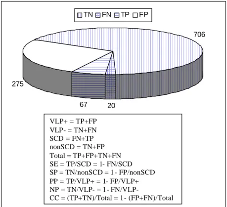
(9) improved upon in this thesis. 1.2.3 Indexes of effectiveness In preventive medicine, as in the case of risk stratification for SCD in post-MI patients, several indexes are used to measure the effectiveness of a particular test. Sensitivity (SE) is a measure of the reliability of a screening test based on the proportion of patients with a specific disease − in this particular case, the patients suffering from sVT/VF and SCD − who react positively (true positives, TPs) to the test. Higher SE implies fewer false negatives, FNs. SE contrasts with specificity (SP), which is the proportion of normals that react negatively (true negatives, TNs) to the test. Higher SP means fewer false positives, FPs. Some other useful parameters to evaluate a diagnostic test are the positive and the negative predictability (PP and NP, respectively), which are related to the group exhibiting and the group not exhibiting VLPs, respectively. To illustrate the previous parameters with numbers from actual cases, a compilation of 6 SAECG studies detailed in [85] will be used. Although not explicit in the paper, some figures and formulas can be easily deduced from the available data and they are included in The results of an individual study can change due to differences in the composition of the group (age, multiple infarctions or some other complications, LVEF, PVCs, etc.), instrumentation, criteria defining VLPs and the follow-up period [141]. SE is obviously wanted to be maximised in any preventive screening test such as VLP detection. If patients detected as VLP+ are going to be considered as at the highest risk for SCD and antiarrhythmic therapy will be implemented (implantation of an expensive ICD, or a drug therapy with possible side effects), then a very high SP must equally be achieved.. Figure 1.2 The 6 studies grouped 1 068 post-MI patients, 342 of them with VLPs (VLP+) and 726 without (VLP-). After a follow-up period (around 1 year), 67 patients from the VLP+ group (TP = 67) and 20 from the VLP- group (FN = 20) developed sVT, VF, or died suddenly. In this global example, the SE, which is the percentage of VLP+ patients from the SCD population, is 77% (67/87). The SP, which is the percentage of VLP- patients from the non-SCD population, is 72% (706/981). The PP, which is the percentage of patients who developed life-threatening episodes from the VLP+ group, is 20% (67/342) and the NP, that is the percentage of non-SCD patients from the VLP- group, is 97% (706/726). The classifications were correct (CC) in 72% (773/1068) of the cases.. 8.

(10) In a newer review of 13 SAECG analysis gathering almost 7 000 patients [17], the SE reported was 62%, SP = 78%, PP = 13% and NP = 98%. The results of an individual study can change due to differences in the composition of the group (age, multiple infarctions or some other complications, LVEF, PVCs, etc.), instrumentation, criteria defining VLPs and the follow-up period [141]. SE is obviously wanted to be maximised in any preventive screening test such as VLP detection. If patients detected as VLP+ are going to be considered as at the highest risk for SCD and antiarrhythmic therapy will be implemented (implantation of an expensive ICD, or a drug therapy with possible side effects), then a very high SP must equally be achieved.. TN. FN. TP. FP 706. 275 67. 20. VLP+ = TP+FP VLP- = TN+FN SCD = FN+TP nonSCD = TN+FP Total = TP+FP+TN+FN SE = TP/SCD = 1- FN/SCD SP = TN/nonSCD = 1- FP/nonSCD PP = TP/VLP+ = 1- FP/VLP+ NP = TN/VLP- = 1- FN/VLPCC = (TP+TN)/Total = 1- (FP+FN)/Total. Figure 1.2 Typical results of SAECG studies for risk stratification of SCD after MI. A review of published reports from 1986 to 1998 [17] reveals that all non-invasive stratification modalities, as well as the EPSs yield a low PP; none has proven useful enough by itself to predict occurrence of sVT or VF. To identify higher risk patients from the initial group under consideration, usually discrete thresholds are fixed for various parameters, for instance, QRSd > 110 ms on SAECG (see Section 2.4.1.). The PP can be increased by using tighter thresholds (e.g. QRSd > 120 ms rather than QRSd > 110 ms), but that could imply a lower SE due to increased FNs. Another solution is to repeat the test at different times during the day, based on the circadian variations of heart. 9.

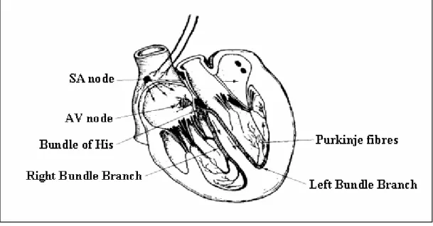
(11) conditions [109]. 1.2.4 SCD model and combination of techniques An accepted model of SCD in coronary heart disease [105] includes a substrate for reentry (provided by a small LVEF and some other factors) [152], which is not selfsufficient to start and propagate a VT, and a trigger mechanism (as PVCs and nsVT) responsible for the initiation of VT. If the substrate exists, a VT can start in the presence of a trigger and, once started, it is self-sustaining. Both the substrate and the triggers are modulated by the autonomic nervous system [186]. Based on this model, a good risk stratification strategy should integrate an assessment of the substrate, the presence of triggers and the function of the autonomic nervous system. At present, EPSs, and/or the presence of VLPs, and T-wave alternans can identify the substrate (although these tests could be independent markers). The triggers are found and quantified by ambulatory ECG monitoring. HRV and baroreflex sensitivity testing can assess the state of the autonomic nervous system. PP and SP can be improved by combining several normal tests [26] [85] [201] [165] [17] [12] [99] [213]. Regardless of the recommended combination of methods, this monographic work will be focused on the VLP detection.. 1.3 Ventricular Late Potentials (VLPs) VLPs are low-amplitude, broad-band-frequency signals, which appear in the HRECG, associated with the arrhythmogenic substrate in some cardiac diseases. Therefore, detection of VLPs can be used as a diagnostic marker. Since these very low level signals are masked by the other components of the ECG and by noise and interference, both in time and frequency domains, its detection remains a challenge. 1.3.1 Origin of VLPs When some region of myocardial (heart muscle) tissue is damaged, conduction delays and blocks can alter the normal electrical activity of the heart. A delayed impulse provokes a late depolarisation after the end of the QRS complex in the ECG signal, which appears as VLPs. ECG and conductive system The waveform resulting from the electrical activity in the conductive system of the heart (Figure 1.4) is called the electrocardiogram, ECG (Figure 1.3). The electrical activity is initiated by depolarisation of the sino -atrial (SA) node, which is the natural pacemaker firing at about 70 times/minute and then, flows through the atria’s fibres to the atrioventricular (AV) node. The horizontal segment preceding the P-wave is the baseline, which is theoretically isoelectric. The P-wave itself represents the atria depolarisation (contraction of the atria). 10.

(12) and is followed by a repolarisation action that does not generate a pronounced potential. Some authors refer that this process coincides in time with the ventricles depolarisation and it is obscured by its resultant potential, the QRS complex. The AV conduction time (PQ interval preceding the QRS complex) should allow sufficient time for complete contraction of the atria and hence the ventricles can be filled with blood before following contraction of the ventricles. AV repolarisation is followed by ventricular depolarisation (QRS complex) through the bundle of His. Finally, the repolarisation of the ventricles is associated to the T-wave.. Amplitude (µV). 1000. R. 500. VLP. P. T. 0. Q. S. -500. -1000. 0. 200. 400. 600. 800. 1000. Time (ms). Figure 1.3 ECG signal (one beat or complex P-QRS-T, healthy 20, Y-lead).. Figure 1.4 Conductive system of the heart. Myocardial infarction and tissue damage The myocardium needs its own blood supply to provide the necessary metabolism for muscular contraction. Oxygenated blood is therefore passed from the lungs to supply 11.

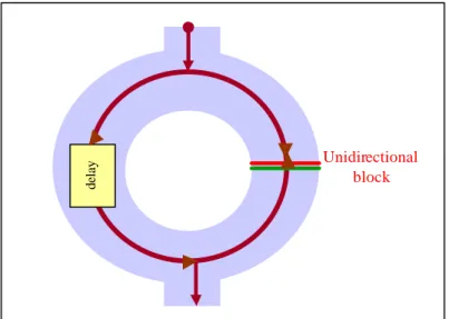
(13) the cardiac muscle via the coronary arteries. This blood then empties into the right atrium to be passed back through the lungs via the right ventricle. An interruption in this supply to a given region of the myocardium provokes an oxygen deficiency, damaging the tissue within the affected area. If an atheromatous artery (with a deposition of plaques, maybe related to a high level of cholesterol) is blocked by a thrombosis, the down-stream blood flow will be insufficient to maintain a normal cardiac metabolism. This condition is called ischemia. If the reduced blood supply is sufficiently low, then the affected tissue will die after a few hours, resulting in a MI, which is the most common cause of myocardial damage. The post-infarction myocardium forms a scar that is inactive electrically (and mechanically). The scar is surrounded by electrically abnormal myocardium, consisting of normal cells alternating with scar tissues and of chronically ischemic cells that are partially depolarised. This abnormal tissue surrounding the scar is the substrate [152] that supports the VT. Re-entrant circuit Although some other mechanisms (like automaticity and triggered activity, which have to do with abnormal impulse formation [85]) can give rise to VT, in the majority of post-MI cases, a conduction phenomenon termed re-entry is responsible. Anisotropy, which is the differences in fibre conductivity in different directions, and depolarisation dispersion are responsible for the re-entrant circuit propagation. Due to a longer pathway of excitation, or a slower conduction velocity, or both [26], a conduction delay may be originated in the damaged area. A damaged area in the myocardial tissue with conduction delays and blocks results in a non-homogeneous dispersion of the impulse between the normal and the damaged parts, which enables the re-entrant electrical circuit.. 12.

(14) delay. Unidirectional block. Figure 1.5 Re-entrant phenomenon in damaged section of myocardium. Figure 1.5 illustrates this re-entrant phenomenon. If an impulse finds two different paths, it will split and take both; if one path is unidirectionally blocked and the other one is sufficiently delayed, due to tissue damage, to allo w recovery of the zone initially blocked, then, a VT can be generated. An impulse is delayed inside the slow conduction path and then re-enters to the near tissue, producing another impulse. Due to the delayed impulse, late depolarisation after the end of the QRS can occur, and fragmented electrical signals can be detected as VLPs at the terminal portion of the high-resolution QRS complex. Abnormal intra-QRS potentials More recently, abnormal intra-QRS potentials have been suggested analogous to conve ntional VLPs, in the sense that they may be arrhythmogenic [143] [146] [24] [44] [81] [80] [79]. It is hypothesised that these potentials may reflect disruption and/or delay in ventricular conduction that is potentially arrhythmogenic. The concept of VLPs might be expanded to include abnormal potentials occurring anywhere within the period of the QRS complex in the HRECG, rather than only the last segment. 1.3.2 VLPs and cardiac care In clinical cardiology, VLPs are found in between 10% and 50% of all cardiac diseases [36] [161]. On the other hand, more than 93% of patients without VLPs are “healthy” people [26], so detection of VLPs is an important diagnostic marker. Detection of VLPs in the HRECG can be used to: • detect post-MI patients prone to sVT and SCD, • evaluate thrombolytic and coronary angioplasty therapy and anti-arrhythmic drugs after MI, • follow progress of patients after anti-tachycardiac surgery, or some other kind of 13.

(15) • •. heart surgery, judge the evolution of some cardiac conditions: cardiomyopathy [70], ischemia [41] [181] [77], myocarditis [32] [102] [178], angina pectoris [6] [205], congenital heart disease [36] [24], study patients with risk factors for cardiovascular disease: hypercholesterolemia [120], hypertension, diabetes mellitus, smoking, heavy drinking [150], and sports practising.. Some other VLP studies deal with Kawasaki disease, antidepressant therapy, sleep apnea syndromes, muscular dystrophy, chronic dialysis treatment, and HIV [21]. Vulnerability to VT and SCD Most of VLP studies reported are concerned with risk stratification for sVT and SCD in post-MI patients [134] [161] [34] [96] [205] [211] [152] [99] [45] [163] [213]. Results summarised elsewhere [26] [85] [17], show that between 12 and 29% of post-MI patients with VLPs conventionally detected, develop sVT or die suddenly, contrasting with only between 0.8 to 4% of those whose HRECG is normal. The SE of this marker varies from 60 to 91%, and SP, from 57 to 79%, in different studies, although high values of SE and SP at the same time are difficult to achieve, limiting the traditional VLP detection applications. Effects of reperfusion and anti-arrhythmic therapies Most cases of MI occur when atherosclerotic plaque in a coronary vessel breaks away from the wall and attracts platelets. The consequent thrombus compromises blood flow. Tissue necrosis begins within 20 minutes of the occlusion. Immediate treatment with an antithrombolytic drug (like streptokinase) or percutaneous transluminal coronary angioplasty (PTCA) is needed to restore blood flow and maintain myocardial function. Effective reperfusion therapy (mechanic or thrombolytic induced [110]) prevents the development of an arrhythmogenic substrate after MI. Numerous papers dealing with the predictive value of VLPs to evaluate the success of thrombolysis or PTCA after MI have been published [41] [103] [110] [114] [125] [144] [181] [77]. In this sense, VLPs are a better predictive marker than the traditional rate of ectopic activity. The absence of VLPs indicates an enhanced ventricular electric activity; successful thrombolytic therapy seems to reduce VLP incidence. If an anti-arrhythmic therapy is followed after a MI, the evolution of the HRECG can help to evaluate, indirectly, its effectiveness. Studies involving drugs as mexiletine, disopyramide, chinidine, propafenone, sotalol, amiodarone and flecainide have been conducted with VLP analysis. Post-operative patients VLP analysis has been used successfully as a post surgical follow-up technique for patients with congenital heart disease. These studies include patients with right 14.

(16) ventriculotomy, operation of Rastelli, and operation of Kawashima, extra-cardiac conducts insertion, tetralogy of Fallot, transposition of the great arteries, aortic stenosis, coarctaction of the aorta and ventricular septum defect [24]. The VLPs have also been used in cases of revascularization and coronary artery bypass grafting. More frequently, VLPs have been used as a follow-up methodology for patients after anti-tachycardiac procedures. Those with VLPs previous to the operation in whom HRECG returned to normal, are more unlikely to develop VT (only less than 10% of them will suffer from VT) [26] [24] [65]. Finally, analysis of VLPs from HRECG may help in the detection of acute rejection after a cardiac transplant [26]. Other studies Patients with risk factors for cardiovascular diseases as hypertension, diabetes mellitus and smoking can be evaluated by HRECG analysis. VLPs are frequently found to be associated with high blood pressure patients. Some studies suggest that diabetes mellitus patients have intra-ventricular conduction disturbances due to diabetes microangiopathy, which can be detected using VLP tests. People who smoke present a high risk for SCD, but no significant differences in VLP incidence have been found to be associated with habitual smokers compared to those who do not smoke. VLPs are not uncommon in sports players and appear related to the left ventricular hypertrophy. 1.3.3 Characteristics of VLPs. Why are they so difficult to detect? The amplitude and frequency characteristics of VLPs, its small duration, and the position they occupy in the HRECG signal, make its detection very difficult. This, coupled with the fact that these signals are very often corrupted by noise and interference, makes VLP monitoring a very challenging problem. Amplitude characteristics VLPs are very low-amplitude signals. These signals appear in the order of 1 to 20µV in the HRECG while using surface electrodes; that is, they are much smaller than the other components of the HRECG (Figure 1.3). For instance, the QRS complex, which “precedes” them, has typical amplitude of 1 mV. Not only the other components of the ECG can mask the VLPs. The noise and interference corrupting the ECG signal can have amplitudes much higher than the VLPs, causing the SNR in the segment of interest (end of QRS complex) to be less than unity. Noise and interference affecting VLPs Noise and interference (Figure 1.6) affect the ECG signal in general, and more severely the VLPs. These disturbances can be associated with the patient, the electrodes, the cables, and the electronic instrumentation system.. 15.

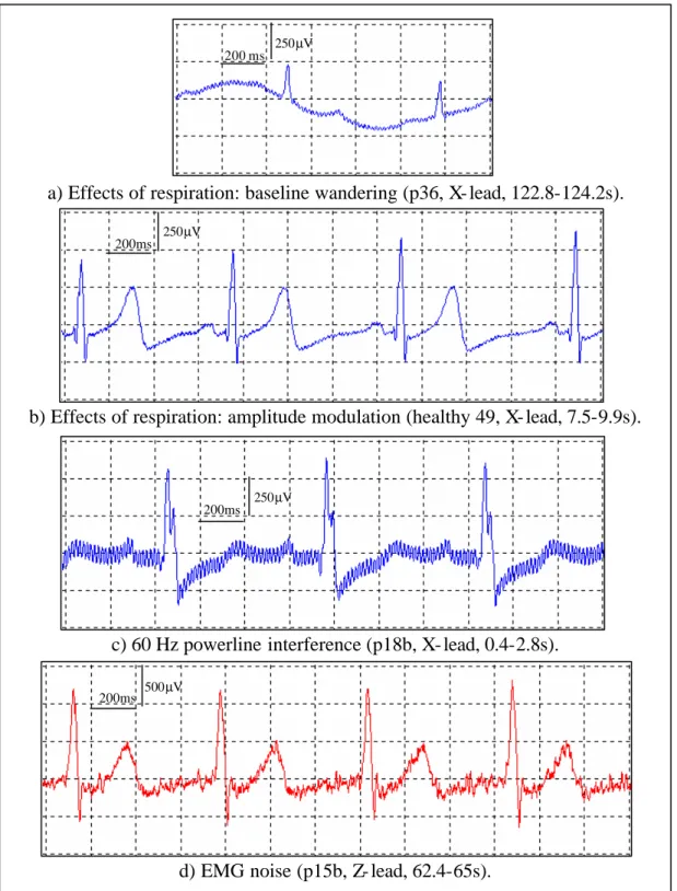
(17) The voluntary or involuntary movement of the patient (due to respiration, coughing, shaking, etc.) provokes changes in the electrode/electrolyte interface, and therefore, generates movement artefacts. The effects of the respiration can be manifested as a baseline wandering (Figure 1.6 a) and /or as an amplitude modulation (Figure 1.6 b). Through the cables, undesirable signals can be electrostatically coupled or electromagnetically induced. An example of the undesirable signals is the 60/50Hz powerline interference (Figure 1.6 c). The most appropriate room for VLPs studies would be a Faraday cage, which provides electrostatic screening. Screening from magnetic influences is more difficult. As a practical solution, the magnetic induction can be minimised by keeping the patient cables close each other (pick up area small) and locating the room as far away as possible from electromagnetic interference sources (e.g. motors, diathermy equipment, etc.). All the electronic components used in the instrumentation for VLPs detection, especially in the first stages of the instrumentation amplifier, should be very low noise. Using these kinds of expensive low noise components, the noise associated to the instrumentation can be drastically reduced but not totally removed. The presence of the instrumentation noise in the ECG signal has the same appearance as the EMG noise. The compound noise corrupting the ECG can be seen as a broadband frequency signal, overlapping with the frequency components of VLPs. Besides, its amplitude normally far exceeds that for the VLPs, leading to a very poor SNR.. 16.

(18) 250µV 200 ms. a) Effects of respiration: baseline wandering (p36, X- lead, 122.8-124.2s). 250µV 200ms. b) Effects of respiration: amplitude modulation (healthy 49, X- lead, 7.5-9.9s).. 250µV 200ms. c) 60 Hz powerline interference (p18b, X- lead, 0.4-2.8s). 200ms. 500µV. d) EMG noise (p15b, Z- lead, 62.4-65s).. Figure 1.6 Noise and interference corrupting the ECG.. 17.

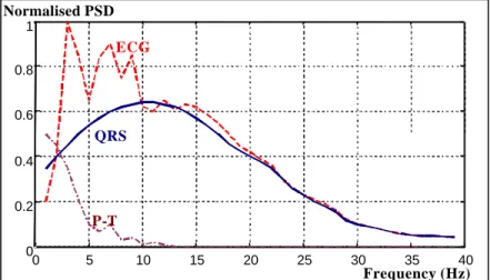
(19) Position of the VLPs in the HRECG Conventional studies of VLPs assume that they are restricted to the last segment of the QRS complex, and initial part of the ST segment, as it was shown in Figure 1.3. More recent theories consider VLPs as a subset of the abnormal intra-QRS signals (notches and slurs) [146] [24] [44] [81] [80] [79]. These theories consider that the areas involved in the VT circuit are mostly activated during the QRS complex and not only in the early ST segment. Therefore, it is necessary to examine a larger portion of the QRS complex to be able to distinguish more precisely arrhythmogenic areas of the myocardium, with the hope that predictability of these tests will improve. Unfortunately, the QRS complex masks considerably these intra-QRS waveforms. Frequency characteristics Traditionally, VLPs have been considered as high frequency signals. Actually, VLPs include components at much higher frequencies than the rest of the waveforms in the conventional ECG. The ECG elements are usually restricted from 0.05 to 100Hz [57], and the most significant spectral components are confined at a smaller range, as it is shown in Figure 1.7. On the other hand, VLPs can carry information even at frequencies of 250 Hz to 300Hz [26]. This suggests the idea that VLPs could be “isolated” from the host ECG by using a high pass filter [182]. Unfortunately, some of the VLP frequency components (around 25 to 40Hz [26], or lower) overlap with those of the conventional ECG. Consequently, using a high pass filter to isolate VLPs from the rest of the ECG is just a compromise Normalised PSD 1. ECG 0.8 0.6. QRS 0.4 0.2. P-T 0 0. 5. 10. 15. 20. 25. 30. 35. 40. Frequency (Hz). Figure 1.7 Power spectral density of the ECG, QRS complex and P and T waves. Difficulties to isolate VLPs Along with the negative SNR in the segment of interest, and frequency overlapping of VLPs with the other components of the ECG, noise and interference, there are some other practical limitations to the isolation of VLPs. The fast transition at the end of the QRS complex preceding the low-amplitude VLP region, is a problem for any filtering 18.

(20) technique because some degree of ringing can appear in the VLP region. In such cases, this ringing can be interpreted as the presence of VLPs, even when they are not present in the original signal (increasing FPs), or they can mask VLPs when present (increasing FNs). In addition, the HRECG is highly non-stationary, affecting the performance of adaptive filtering and other conventional filtering techniques. Current techniques for detection of VLPs, in general, pose the following limitations: • Averaging of a significant number of beats is required. • Inability to operate properly with non-stationary data. • Inability to obtain specific beat-to-beat variability information. • Analysis constrained to the end of the QRS complex. • Poor SE and SP in VLP detection (Section 1.2.3).. 19.

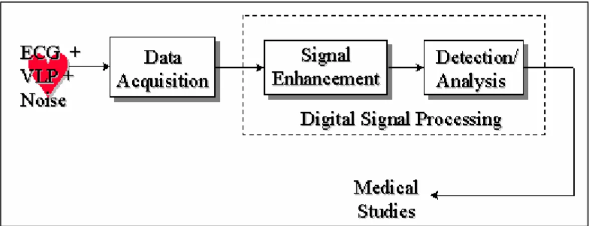
(21) Chapter 2 - Current clinical and research approaches 2.1 Introduction Low-level signals, directly recorded from ischemic regions of a canine model of MI, were described for the first time in 1973 [25]. This was followed in 1978 with the first recording of VLPs, again in a canine MI model, using surface electrodes [46]. In the same year, studies on VLPs recorded from the human endocardium were published [104]. In 1981, Simson introduced the basis for non-invasive studies of VLPs in man in the time domain [182], which was adopted as a standard ten years later [26]. During the 1980’s, VLP studies in the frequency domain were essayed [49]. More recently, VLP studies in the time-frequency plane were proposed [121].. Figure 2.1 System for detection and analysis of VLPs. The detection and analysis of the VLPs require special instrumentation or HRECG acquisition systems, and digital signal processing techniques for the enhancement and analysis of the signal of interest (Figure 2.1). Once the ECG signal is acquired, by using high-resolution equipment, a noise diminishing strategy has to be applied in order to obtain the relevant information associated to the presence (or absence) of the VLPs.. 2.2 Instrumentation requirements The first stage in any ECG acquisition is the electrode-lead system. This is followed by analog conditioning circuitry that includes differential amplification, common mode rejection and filtering. Analog-to-digital conversion is then performed to provide a signal that is suitable for sophisticated signal processing and computer analysis. Electrodes Electrodes are transducers that convert the ionic currents in the biological system to electronic currents compatible with the electronic instrumentation. The electrograms recorded during invasive EPSs need special internal electrodes that are placed by. 20.

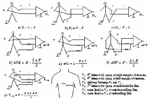
(22) means of catheters [220] [118] [133] [90] [197]. Some other “non-invasive” VLP studies have successfully used multipolar intra-esophageal electrodes. However, most VLP recording systems use surface electrodes placed on the skin. The surface electrodes of choice for VLP studies are silver/silver chloride (Ag/AgCl) [26], which are non-polarizable, low-noise, very stable, and provide a low half-cell potential. Good skin preparation, including cleansing and abrasion, is needed before placing the electrodes. In addition, the use of an electrolytic paste will help to reduce the contact impedance. Published standards [26] state that “ideally, electrode impedance should be measured and be less than 1000 Ω.” However, it is not clear if they refer to the contact impedance or to the overall electrode/skin impedance. In addition, the frequency at which impedance should be measured is not mentioned. Lead systems Amplitude, polarity, and even duration of the ECG components depend on the position of the electrodes on the body. Therefore, these characteristics depend on the lead system used. The most common ECG leads are reviewed in Figure 2.2. This standard 12-lead system includes three basic bipolar leads (D1, D2, and D3), three unipolar augmented leads (aVR, aVL, and aVF), and six pre-cordials or chest leads (V1 to V6). This system has been used for VLP detection [115] but not very often.. Figure 2.2 12-lead system commonly used in clinical ECG.. 21.

(23) When a tri-dimensional representation of the ECG is required, as in the case of VLP studies, an orthogonal system is normally preferred. The standardised lead system for VLP studies [26] is the orthogonal bipolar XYZ system [182] shown in Figure 2.3.. Figure 2.3 XYZ orthogonal lead system recommended for VLP studies. The electrodes for the X-lead are placed at the fourth intercostal space in both midaxilary lines (the left electrode is connected to the non-inverting input of the amplifier). The Y-lead takes the potential between the left iliac crest (non-inverting electrode) and the intersection of the first intercostal space with the left midclavicular line. The Z-lead is measured between the chest and the back, placing the non-inverting electrode at the fourth intercostal space at left margin of sternum, and the inverting one, on the reflection of the non-inverting on the back. In most of the VLP studies, the filtered leads are combined to form a cardiac vector magnitude [26], V =. X 2 +Y 2 + Z 2 ,. Eq. 2.1. as a sub-optimal method of data reduction [33]. In order to obtain computational simplicity, the sum of the absolute values has been used in some studies [33] [98],. S= X +Y + Z .. Eq. 2.2. The frequency content in ECG signals depends on the lead used. Established criteria using a lead system cannot be applied to others. However, quasi-equivalent systems have been found. For example, modified orthogonal systems, precordial leads V4, V6 and V2, and individual orthogonal leads (X, Y and Z) [33] [193] may improve the sensitivity to detect ventricular arrhythmia due to better SNR compared to the vector magnitude V. To evaluate spatial localisation of VLPs and noise, systems using multiple 22.

(24) unipolar thoracic leads, have been developed [33] [64]. Amplification The first stage in the ECG amplifier should be a differential one with a high gain (Ad) and a high common-mode rejection ratio (CMRR) [142]. In a conventional electrocardiograph, the gain is typically 1 000, but it may be even higher in a HRECG system. To obtain a high value of Ad, several amplifier stages are needed. The first stage should have a gain (A1) as high as possible (without saturation), and it should be very low noise (N1→0) in order to minimise the total level of the instrumentation noise referred to the input (Ns ). The total noise Ns can be expressed as a function of the gains Ai and the individual noise Ni of every i-th stage [54]. In the case of 3 stages,. N 1 A1 A2 A3 + N 2 A2 A3 + N3 A3 . Eq. 2.3 A1 A2 A3 Ns can be measured by shorting the inputs of the first stage and should be <1µV rms [33]. Ns =. The total root-mean-square (rms) input noise of an amplifier involves the thermal noise due to the real part of the source impedance (electrode impedance plus contact resistance) and the inherent amplifier noise, which is frequency-dependent. This inherent amplifier noise includes the effect of the equivalent input noise voltage source (~ 10nV Hz ) and the equivalent input noise current generator (~ 1 pA Hz ) [142]. In most cases, the equivalent electrode input noise current is the primary component due to relatively high value of the source impedance. In conventional ECG, the CMRR is typically 100dB, that is, a ratio of 1:100 000 [57]. However, in the detection of VLPs, CMRR should be at least 120dB (1:1 000 000) [33] to provide adequate powerline frequency attenuation. This level of CMRR requires an exceptional amplifier design, employing such techniques as power supply bootstrapping and guarding. To complete the recommendations for the analog front-end, the linearity range for the input signals should be not lower than ±2.5mV. In addition, the calibrating voltage should have a precision of ±2% [26]. Frequency response The minimum bandwidth (B w = fh – fl ) of the systems used to detect VLPs, should be between 0.5 and 250Hz, contrasting with the B w between 0.05 and 100Hz used in conventional ECG. In VLP frequency-domain studies, B w should be even wider (0.05~300Hz) [57] [26]. A high-pass filter (HPF) eliminates DC (direct current) offset voltage of the electrodes and the amplifiers, and attenuates the baseline wandering and other low frequency component noise. An analog low-pass filter (LPF) reduces the high frequency components of the noise affecting the ECG and acts as an antialiasing filter prior to sampling [145]. Active Bessel filters are the filters of choice because of their 23.

(25) smooth transfer function [142] and good transient response. In VLP studies, the use of notch filters to remove powerline frequency interference is not recommended [26]. This is due to the poor phase response close to the null that can severely distort the VLPs due to the close proximity of the large QRS complex. However, some other techniques to reduce 60Hz interference from HRECG records have been evaluated [98]. Analog-to-digital conversion To allow for digital signal processing, necessary to resolve the VLPs, the ECG signal must be digitised. Associated with analog-to-digital (A/D) conversion, the phenomenon of aliasing must be avoided [145] [130]. This aliasing is a frequency ambiguity in the sampled signal that makes accurate reconstruction impossible. To prevent aliasing, the sampling frequency (fs ) should be, greater than, twice the highest frequency component in the original analog signal. The minimum sampling frequency fs recommended for VLP studies is 1kHz. Using this minimum demands that the analog signal frequency components higher than 500Hz (fs /2) should be sufficiently attenuated before entering the A/D converter. If fs is increased (for example, to 2kHz), then the specifications of the analog filtering can be reduced, that is, the transition band can be wider, but memory and computation power requirements will be more demanding. Normally, an analog low-pass filter with a cutoff frequency around 250 to 300Hz is used before the A/D converter. However, no mention of the order of the filter is given in the literature. In the conventional quantitative ECG, the quantisation interval or step size Vlsb , that is, the difference between 2 quantisation levels in the A/D conversion, should be not bigger than 5µV [57]. However, in the HRECG used to detect low-level VLPs, this resolution should be increased to at least 2.5µV [26], although some research has claimed good results using a resolution of only 10µV [193]. To achieve the recommended resolution, the A/D converter should quantise to 12 bits or better (b ≥ 12) [26]. The associated quantisation error [145] [193] [130] can be assumed to be an additive white noise source with a uniform distribution and standard deviation given by σ q = Vlsb. 12 .. Eq. 2.4. The maximum analog input of the A/D converter (Vmax ) is dependent on the resolution (number of bits, b) and the gain (Ad) of the system. The following equations can be useful in the design process:. AdV p ≤ Vmax AdVlsb ≥ Vmax 2 b. .. Eq. 2.5. In Eq. 2.5, Ad is the gain of the electrocardiograph (~ 1 000), Vp is the peak voltage (~ 2-. 24.

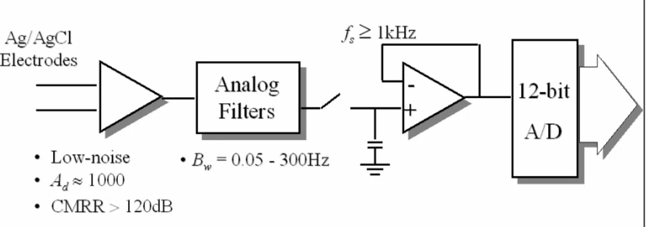
(26) 4mV) of the ECG signal (QRS complex), Vmax is the maximum input voltage of the A/D converter (normally ±5V), Vlsb is the quantisation level (Vlsb ≤ 2.5µV), and b is the number of bits of the A/D converter (b ≥ 12). The A/D conversion time is not a critical parameter. It depends on fs , and on the flexibility of the system. For instance, using an orthogonal lead system, samples from X, Y and Z channels should be concurrently taken. Depending on the sampling process, and the characteristics of the A/D converter (b and conversion time), sample and hold circuits (S/H) may be necessary. For example, in the case of the orthogonal lead system, 3 S/H with a common control input should be used to avoid any time skew between channels. Safety As in any other biomedical equipment that is connected to a subject, safety is of paramount concern. Consequently, the usual requirements regarding leakage current and patient risk current apply. In Canada, these requirements are defined by the Canadian Standards Association (CAN/CSA-C22.2 No. 601 for Medical Electrical Equipment). It is interesting to note that in the case of equipment used in VLP studies, no special protection against defibrillation discharges is required [26]. Summary Fig. 2.4. reviews the requirements for the instrumentation used in VLP studies. Only one channel is shown, but normally the system for VLP detection needs more. For example, to use the XYZ orthogonal lead system, 3 channels are needed; a fourth channel acquiring the common mode signal may be used to implement an adaptive canceller (Section 2.3.4). In these multichannel systems, the interchannel cross-talk separation should be higher than the dynamic range allowed by the A/D converter, which (in dB) is approximately 6 times the number of bits b. For instance, if a 16-bit A/D converter is used, the recommended interchannel cross-talk separation is 100dB [33].. 25.

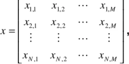
(27) Figure 2.4 Instrumentation requirements for VLP acquisition (one channel). In summary, instrumentation for VLP systems requires a differential gain in the order of 1 000, a CMRR higher than 120dB [33], and a minimum bandwidth between 0.5 and 250Hz, although in frequency-domain studies must be between 0.05 and 300Hz [26]. Data must be sampled at least 1 000 times per second, and the A/D converter must have at least 12 bits to achieve a resolution better than 2.5µV [26].. 2.3 Signal enhancement techniques 2.3.1 Introduction The signal (x) acquired using the HRECG, can be modelled as a desired signal (s), which includes the ECG signal and the VLPs if present, and an additive 1 noise (n), representing all the different sources of noise and interference affecting the ECG. To enable the reliable detection of the low-level VLPs, digital signal processing techniques must be applied to enhance the SNR (Figure 2.5). The output (y) of such enhancement block is an estimation ( ŝ ) of the desired signal, which can be seen as a combination of the signal s and some remaining noise θ. If the enhancement block is a linear time invariant system [145] characterised by an impulse response h[k], then the output y[k] can be expressed by the convolution of the input x[k] with h[k], y[ k ] = x[ k ] ∗ h[ k ] =. ∞. ∑. m = −∞. h[ m ] ⋅ x[ k − m ] =. ∞. ∑ x[m] ⋅ h[k − m] .. Eq. 2.6. m = −∞. If X(f), Y(f) and the frequency response H(f) are the Fourier transforms [145] of x[k], y[k] and h[k] respectively, then Eq. 2.6 can be written in the frequency domain as. 1. The assumption that all noise is additive can be fairly accepted, although there may be some multiplicative noise like the amplitude modulation shown in Figure 1.6 b.. 26.

(28) Y( f ) = X ( f )⋅ H ( f ) .. x = s+ n. s +. Enhancement Strategy. Eq. 2.7. y = sˆ = s + θ. n. Figure 2.5 Signal-to-noise ratio enhancement. Most enhancement strategies used with ECG signals assume “quasi periodicity”, that is, that the PQRST complex of one heartbeat is almost the same as the other [14] [53]. Therefore, some segments of interest can be isolated from every heartbeat by using a temporal reference (fiducial mark) like the QRS complex. A QRS detector [73] [106] [71] is the cornerstone of these algorithms; it is crucial for the coherent averaging technique [168] [130] [33] and for the segmentation of the ECG signal.. Figure 2.6 Isolation of segments of interest from the ECG sequence.. Figure 2.6 shows an example of how the segments of interest (dashed boxes) around the fiducial marks (vertical lines) can be isolated from the whole ECG sequence by using a QRS detector. If M is the number of samples to be isolated and N is the number of heartbeats included in the analysis, the new signal x can be written in a matrix format as.  x1,1 x 2 ,1 x=  M   x N ,1. x1, 2 x 2, 2 M x N ,2. L x1, M  L x 2, M  , L M   L x N,M . Eq. 2.8. 27.

(29) where every row represents a different heartbeat and every column represents a different sample. The quality of a particular segment of the HRECG signal can be expressed in terms of several parameters. Some of the most important parameters to qualify a sequence y are the variance of noise σθ2, which represents the noise power [122] and is calculated by using Eq. 2.9, and the bias bθ calculated by Eq. 2.10 [123] [160]. Here, the bias is defined slightly unconventional (including modulus sign) to consider the HRECG as a signal with a definite time structure [123]. Another important parameter is the SNR, which can be estimated by Eq. 2.11.. σθ = 2. 1 M. ∑ (θ[ j ] − θ) M. 2. Eq. 2.9. j =1. bθ =. 1 M. M. ∑ θ[ j ]. Eq. 2.10. j =1 M. ∑s [j] 2. SNRy =. j =1. Eq. 2.11. M. ∑ θ [ j] 2. j =1. In Eqs. 2.9-2.11, M represents the total number of samples of the segment to be evaluated, θ is the underlying noise in the signal y, and θ is the mean value of θ. The subscript j identifies the j-th sample of the affected parameter and s is the ideally pure signal, which is unfortunately unknown. It is very difficult to obtain a very low variance and a very low bias at the same time in the VLP region after applying a particular enhancement technique in a practical situation (with a reduced number of beats N). Nevertheless, several approaches have been followed with various degrees of success. The techniques implemented for noise reduction in VLP studies include coherent averaging, optimal filtering, adaptive filtering and more recently, denoising with Wavelets. 2.3.2 Coherent averaging In commercial HRECG systems for clinical use, the noise reduction strategy of choice is coherent averaging. To implement this technique, N heartbeats (normally 50 < N < 300 [26]) are aligned by using temporal references (fiducial marks) and then averaged. This process can be described by y j = xj =. 1 N 1 N 1 x i, j = ∑ s i, j + ∑ N i=1 N i=1 N. N. ∑n. i, j. ,. Eq. 2.12. i =1. 28.

(30) where N is the total number of heartbeats (isolated segments), yj is the j-th sample of the output, and xi,j represents the j-th sample of the i-th isolated segment [33]. The complete output sequence is equivalent to averaging each column of Eq. 2.8. Assuming that the noise n is additive, uncorrelated with the signal s and stationary, and the signals of interest (VLPs) do not change from beat to beat and they are accurately synchronized with the fiducial marks, the resulting signal y has a variance and a voltage SNR given by [54] [33], σ = x , N 2. σy. 2. SNRy = SNRx N .. Eq. 2.13 Eq. 2.14. This noise reduction due to averaging is illustrated in the right side of Figure 2.7. The variance of the output signal y decreases proportionally to the number of averaged normal heartbeats N (PVCs have to be eliminated before averaging). Therefore, the voltage SNR improves by a factor of N . Unfortunately, in a practical situation, none of the conditions assumed above are absolutely fulfilled. QRS. s1. VLP. s2 M. +. n1. +. n2 M. τN. t iN. t Nf. +. ⇓. ⇓. s. nN. rounding. +. n. Figure 2.7 Coherent averaging for VLP enhancement showing the trigger jitter effect.. 29.

(31) Figure 2.7 (left side) also illustrates the effect of variability of the distance τ from the initial sample or trigger of the analysis window (see Figure 2.6) to the position of the VLPs, represented here by a step function. variability is known as trigger jitter [169] and is due to the variability of ti and tf .. This. The distance ti between the initial point (trigger) and the theoretical fiducial mark, represented by the peak of the triangular waveform, can vary because of alignment imperfections in a noisy environment [73] [106] [203], and because of the decimation in time of the system with a fixed sampling rate [192]. To minimise this effect, highresolution QRS detectors have been developed [171]. Nevertheless, the distance tf from the fiducial mark to VLPs can vary considerably (~ ms) from beat to beat [51] [192] [112] [113] [94] [40] [152] [180] [196] [42]. Assuming that ti and tf are random variables, normally distributed with zero mean and non-correlated [54], τ, which represents the total misalignment, will be normally distributed with zero mean and variance στ2 equal to the sum of the individual variances of ti and tf. As a consequence, the misalignment in the signal averaging process yields a further low-pass filtering effect depicted as rounded edges of s in Figure 2.7. This low-pass filtering effect [169] [54] [171] [130] is characterised by the frequency response of the trigger jitter H tj ( f ) ,. (. H tj ( f ) = exp − 2 π2 σ τ f 2. 2. ).. Eq. 2.15. cutoff frequency. (Hz). 500 450 400 350 300 250 200 150 100 50. 0. 1 0.5 1.5 standard deviation of the alignment error (ms). 2. 2.5. Figure 2.8 Cutoff frequency of the trigger jitter equivalent filter.. 30.

(32) It can be found, from Eq. 2.16, that the cutoff frequency of the trigger jitter equivalent filter, shown in Figure 2.8 , is fh =. ln 2 . 2 πστ. Eq. 2.16. 2.3.3 Optimal filtering and weighting averaging To minimise the mean square error (MSE), that in this case is the mean square of the output noise θ in Figure 2.5, Wiener filter theory can be applied. Minimising the expectation of θ2 with respect to h[k] yields the optimal filter (in the sense of minimum square error). In the frequency domain, this can be expressed as. H opt =. Φ ss ( f ) , Φ ss ( f ) + Φ nn ( f ). Eq. 2.17. where Φ ss and Φ nn represent the power spectral densities (PSDs) of the signal s and the noise n, respectively [87]. To design the optimal filtering, these PSDs have to be estimated from the available signal x. Filters based on Wiener’s theory assume that signal and noise are not correlated and they can be described using statistics [188] [122]. In addition, the optimal filter Hopt(f) considers the data to be quasi-stationary. When the signal (or noise) is non-stationary, an extended time-varying form of an A Posteriori Wiener Filter (APWF) can be useful. To estimate the signal and noise PSDs from the ensemble, the power spectrum of the ensemble must be used along with the averaged power spectra of each record. From these parameters the optimal filter response can be obtained. However, Hopt(f) introduces a bias in sˆ( t ) that is unacceptable at low SNR. In the power spectrum of the ensemble, the averaged power spectra of each record are smoothed to reduce their variances; this attenuates the bias, but fidelity in signal estimate may be compromised [122]. Recently Lander and Berbari [122] [123] approached the VLP enhancement problem by means of an APWF in the time-frequency (t-f) plane [93]. The major problem of this technique is the adaptation of the t-f structure of the filter to that of low-level VLPs. However, they used a t- f signal representation based on a smoothed version of shorttime Fourier Transform (STFT) and obtained an acceptable SNR by using only 64 heartbeats. Similar results were obtained by Rakotomamonjy et al. [160] by using an optimal wavelet-domain filter [111]. In both works mentioned above, [123] and [160], the filter is optimal in the mean square sense. This means that errors in the high-amplitude QRS complex and in the lowamplitude VLP segment are treated equally [160]. While this approach will produce an optimum result in terms of the overall ECG, the enhancement may be biased by the. 31.

(33) large amplitude QRS segment at the expense of the VLPs. In addition, the additive noise is assumed to be perfectly white, which is not the case in a clinical situation. Another method for improving the SNR of an averaged ECG can be based on a simple statistical model that considers VLPs as Gaussian processes with standard deviation α. The optimal one-weight (ρ) filter can be estimated from the beat ensemble using the maximum likelihood estimator of the ensemble correlation [9] [10]: ρ=. α2 α 2 + σn. 2. .. Eq. 2.18. The noisiest intervals of the signal have weights ρ close to 0 and the intervals where VLPs occur have weights ρ close to 1 (weighted averaging). In certain situations the 2 noise is non-stationary so an estimate of the noise variance σ n for each beat is required [11]. This increases the computational complexity considerably. 2.3.4 Adaptive filtering In VLP studies, generally the signal is non-stationary with unknown PSD. Consequently, an adaptive filter, which can continuously adjust itself to perform optimally under the changing circumstances, may be a good solution [127] [87] [130]. Indeed, different adaptive filter implementations such as noise cancellers have been reported for VLP enhancement [51] [195] [199] [40] [137] [202]. These use an additional channel to provide signal enhancement. The basic adaptive filtering structure used as a noise canceller is shown in Figure 2.9. Here, x represents the primary input, while r represents the additional reference input. n and nr represent additive noise, added to signals s and sr respectively. Signal and noise are uncorrelated in x and r. y2 is the output of the inverse filter, whose M coefficients W are adapted by minimising the error ε, following some correction criterion. Several algorithms or correction criteria for the optimisation have been developed [87], but the most dominant ones are the least mean squares (LMS) algorithm, and the recursive least squares (RLS) algorithm. Both have been used for VLP enhancement.. 32.

(34) x = s+ n. y1 = ε. + -. r = s r + nr. y2. W (Z ) Correction criterion. Figure 2.9 Adaptive filter enhancing set-up. The LMS algorithm is a simple iterative technique to minimise the MSE between x and r. This algorithm can be described by Wk +1 = Wk + 2ε k Ak µ , where Wk = [W1 [k ]. Eq. 2.19. W 2 [ k ]L WM [ k ]] is a set of filter weights at sample k, T. Ak = [ A1 [k ] A2 [ k ] L AM [ k ]] = [rk rk −1 L rk − M ] is the input at sample k, εk is the error at sample k, and µ (step-size parameter) is a scalar that controls the stability and convergence of the algorithm. T. T. For larger µ, the convergence is faster. However, to ensure stability, µ should be lower than 1/γ, where γ is the largest eigenvalue of the autocorrelation matrix of r. The time constant for convergence is 1/ (4 γ µ) [87]. Normally, the rate of convergence of the RLS algorithm is faster than the LMS algorithm, but its complexity is increased. Here, Pk −1 Ak Gk = λ + Ak T Pk −1 Ak P − Gk Ak T Pk − 1 , Pk = k − 1 λ. Eq. 2.20. ε k = xk − Ak T W k − 1 Wk = Wk −1 + ε k Gk where G is the gain vector, ε is the true estimation error, P is the error correlation matrix (initially P0 = I/C, where C is a small positive value and I is the Identity matrix M×M) and λ (forgetting factor) is a positive scalar (λ ≤ 1, close to 1) to ensure that data in the distant past is forgotten in order to afford the possibility of working properly in 33.

(35) a non-stationary environment. For λ < 1, the past data are attenuated exponentially, with the result that the present data have a larger influence on the updating computation than the past data. From Figure 2.9, two different cases can be analysed [206]: 1. nr is correlated in certain way with n, but sr is null or it is not correlated with s. 2. sr is correlated in certain way with s, but nr is not correlated with n. In the first case, the enhanced signal appears as y = y1 = ε, and in the second case, y = y2. An example of case 1 is the powerline interference cancellation from an ECG signal, provided a reference that resembles that interference [206]. Using custom-designed electrodes, which provide separate electrode contacts [51] [40], the second case can be implemented. A particular implementation of the second case can be achieved by using a delayed version (1-sample or 1-heartbeat [202]) of the primary input x, as a reference. This specific set-up is known as adaptive line enhancing (ALE) [87] and it was recently declared unsuitable for VLP enhancement [137], at least in the simplest way it was implemented. Conventional adaptive filtering faces serious limitations to remove wide band noise from the ECG because of the adverse dynamic range of this kind of signal, that includes highamplitude segments such as QRS complex (~mV) followed by very low-amplitude segments such as the VLPs (~µV). Two different ways to deal with this problem are the hybrid t-f adaptive filtering and the time-sequenced adaptive filtering (TSAF) [51] [195]. In hybrid t-f adaptive filtering [199], the signal is divided in several frequency bands and each band is adaptively filtered before recombining to produce a final output. The TSAF is an implementation that may enhance signals that occur on an event basis, like the ECG signal, and it has been used for VLP enhancement [51] [195] [1] [214]. In the segment of interest, each sample point has an associated adaptive weight vector. This weight vector is updated only when the corresponding sample is current at the subsequent regeneration. The TSAF acts as a signal enhancer that converges to a rapidly time-varying solution. 2.3.5 High-Order Spectrum High-Order Spectrum techniques, particularly second order or bispectrum, have also been suggested by Speirs [194] for VLP studies. This technique may improve the SNR based on the zero higher order spectra (of order greater than 2) of Gaussian noise, which is the most predominant in the ECG signal. Spaargaren and English [173] [176] have recently introduced some refinements for practical use in VLP enhancement. 2.3.6 Denoising with Wavelets In the last 5 years, wavelet transform denoising techniques have been applied to obtain 34.

(36) reasonably good results for analysis of VLPs. A group of the University of Patras, Greece, has published a series of papers [43] [149] [152] showing the potential advantages of this technique compared to the more traditional ones. Some other authors have successfully used this procedure [111] [7] [160], which will be addressed in considerable detail in Chapter 3. In the implementation of this technique for VLP enhancement, some practical limitations appear. It has been reported that the denoising errors tend to concentrate within the QRS complex [200], which is precisely the segment of interest in VLP enhancement. In addition, the variance (noise power) in the “isoelectric” segment of the ECG can be drastically reduced, but at the same time, the VLP components may be considerably attenuated [160]. While applying wavelet shrinkage, like in more conventional types of filtering, certain ripple appears in the discontinuities of the signal, which is the case of the segment of interest. This is due to the lack of translation invariance of the wavelet transform but it can be solved by applying a second generation of wavelet denoising.. 2.4 Detection/analysis After signal enhancement, a method to obtain relevant information on VLPs must be applied. Traditionally, the most common approach is time-domain analysis, although some research deals with the frequency domain and more recently, with t-f representations. 2.4.1 Time domain In 1991, a Task Force Committee between the European Society of Cardiology, the American Heart Association and the American College of Cardiology established standards for data acquisition (Section 2.2) and analysis of VLPs [26]. Most details in these guidelines are given for the time-domain analysis. The Task Force Committee recognised the filtered QRS complex as one standard [26]. This filtered QRS complex is the vector magnitude V of Eq. 2.1, where X, Y and Z, are the coherent averaged orthogonal leads of Figure 2.3 after being high-pass filtered to attenuate the low frequency components of the ECG. Simson [182] proposed a bi-directional four-pole Butterworth high-pass recursive digital filter (cutoff frequency of 25 or 40 Hz) to avoid ringing and to ensure that the onset and offset of the filtered QRS coincide with those in the original signal. Figure 2.10 shows the performance of a conventional unidirectional filter and the one proposed by Simson [182] and accepted as standard [26]. Unfortunately, the non-linear phase response of the high-pass Butterworth recursive digital filter is a source of signal. 35.

(37) distortion. This weakness gave rise to some studies [82] [20] to find a linear phase equiva lent filter. The noise in the isoelectric segment of the filtered QRS complex has to be reduced to less than 0.7 µV rms if the cutoff of the high-pass bidirectional filter is 40Hz, or to less than 1µV rms if the cutoff is reduced to 25Hz [26]. This noise is measured over an interval longer than 40ms in the ST or TP segment [26]. For some other types of filters or cutoff frequencies, there are no established guidelines. 500. 500. Test signal. Test signal. 0. 0. Filter direc. Filter direc. -500. -500 -50. 0. 50. 100. 150. 200. 80. -50 80. 60. 60. 40. 40. 20. 20. 0 -50. 0. 50. 100. 150. a) Conventional filter.. 200. 0 -50. 0. 50. 100. 150. 200. 0. 50. 100. 150. 200. b) Bi-directional filter.. Figure 2.10 Performance of conventional and bi-directional high-pass filtering [182]. The reduction of noise in the isoelectric segment is crucial for a successful determination of the onset (initial point) and offset (final point) of the filtered QRS complex. Standards [26] propose the automatic estimation of the initial and final points of the filtered QRS complex and its visual verification along with a manual adjustment feature. Onset (offset) is estimated as the midpoint of a 5ms moving window, advancing from left to right (from right to left), in which the mean voltage surpasses the mean plus 3 times the standard deviation of the noise in the isoelectric segment [182].. 36.

(38) Figure 2.11 Features in VLP time-domain analysis (p38). From the filtered QRS vector magnitude, after estimating the onset and offset, three parameters or features can be measured to determine the presence of VLPs (. Figure 2.11):. • • • • • •. Duration of the filtered QRS (QRSd), measured from the onset to the offset. Low-amplitude signal duration (LASd), measured from the offset backward to the point where the signal reaches 40µV. Root mean square voltage (RMS40), which is the rms voltage from the offset to 40ms into the QRS (shadowed in. Figure 2.11).. Every laboratory should establish its own normal parameters to define the presence or absence of VLPs. An example cited in the standards [26] fixes the criteria to define a VLP positive test as: QRSd > 114ms, LASd > 38ms, and RMS40 < 20µV. Balance between sensitivity SE and specificity SP (Section 1.2.3) can be controlled by selecting one, two or three of above three criteria at the same time [216].. 37.

(39) shows an example of a patient with the three time-domain criteria reached, although QRSd and LASd are very close to the thresholds mentioned above. Figure 2.11. From the LASd and RMS40 parameters, some morphology information can be extracted indirectly, but signal morphology around the terminal part of QRS includes a significantly larger amount of information. To extract more information, artificial neural networks (ANN) have been used in recent works [92] [112] [216] [167] [89] [117] [214], achieving better SE and SP in time-domain VLP analysis. To detect and analyse VLPs, fractal dimension analysis has also been used. In these studies, Escalona and collaborators [72] [132] have used the fractal dimension of the VLP attractor (3-D VLP geometric curve) to quantify the degree of complexity of VLPs in the time domain. Time-domain analysis can isolate the VLPs in the ECG signal. It provides less false positives (FPs) than other methods, it has the best reproducibility [31] [209] and its basic guidelines are standardised [26]. Nevertheless, the noise level and the number of averaged beats affect time-domain analysis definition and high-pass filters can introduce artificial signals, which affect the final results. Furthermore, this approach cannot be implemented on patients with bundle branch block. These limitations warrant the development of other approaches. 2.4.2 Frequency domain Parallel to the time-domain, frequency-domain techniques for VLP analysis have been established. Most studies in the frequency domain are based on Fourier transformation and the periodogram, although some researchers have used the Fast Harley Transform [32], maximum entropy spectrum estimation [179] [210], time variant auto-regressive spectral analysis [39], spectral turbulence analysis [134] [84] [209] and acceleration spectrum analysis [208] [209]. In the frequency domain, stationary signals can be described by means of the amplitude (|X(f)|) and phase (θ(f)) of the sine waves in which they can be decomposed. To obtain the equivalent frequency domain representation X(f) of a signal, given its description in the time domain x(t), the Fourier transform (F{⋅}) is used (Eq. 2.22). Inversely, the inverse Fourier transform (F-1{⋅}) transforms a signal from the frequency domain into the time domain (Eq. 2.23). X ( f ) = F {x(t )} =. ∞. ∫ x(t )e. − j 2 πft. dt = X ( f )e jθ( f ). Eq. 2.21. −∞. x (t ) = F. −1. ∞. {X ( f )} = ∫ X ( f )e j 2 πft df. Eq. 2.22. −∞. A useful tool for VLP spectral analysis is the power spectral density (PSD).. This. 38.

(40) parameter gives the density of power on the frequency axis. The PSD of the signal x (Φ xx ) is defined as the Fourier transform of the autocorrelation function (φ xx ). ∞. Φ xx ( f ) = F{φ xx } =. ∫ φ (k )e. − j 2 πft. xx. dt. Eq. 2.23. −∞. φ xx (m) = E [x(i − m)x (i )]. Eq. 2.24. For sampled signals x[m] (with sampling frequency fs and M samples), the representation in the frequency domain X[k] can be obtained by using the discrete Fourier transform (DFT), efficiently calculated by means of the Fast Fourier Transform (FFT) algorithm in most implementations [145]. It should be noticed that the spectrum of the sampled signal is the spectrum of the original signal repeated at every multiple of the sample frequency fs . The inverse operator, IDFT, transforms the sequence X[k] back into the time domain x[m]. M −1. X [k ] = DFT {x[m ]} =. ∑ x[m]e. − jkm. Eq. 2.25. m= 0. x[m ] = IDFT {X [k ]} =. 1 M. M −1. ∑ X [k ]e. jkm. Eq. 2.26. k=0. The autocorrelation can be estimated by 1 φˆ xx [m ] = M. M −i −1. ∑ x[m + i]x[i] .. Eq. 2.27. n= 0. The frequency resolution ?f that can be provided by the DFT of an M-sample signal, sampled at a frequency fs is given by,. ∆f =. fs . M. Eq. 2.28. The number of samples M of the signal x mostly depends on the segment of interest. The starting point and the length of the window also constitute polemic issues in the literature [23]. The analysis period has been extended towards the T wave, covering the ST segment to improve the frequency resolution of the FFT. The starting point of the interval to be investigated can be determined by using a single threshold in the timedomain signal (e.g. 40µV) or the derivative of it (e.g. 5mV/s) [23] [189].. 39.