TítuloExperimental study and random forest prediction model of microbiome cell surface hydrophobicity

Texto completo

(1)Expert Systems with Applications. 2017; 72: 306-16. Experimental study and random forest prediction model of microbiome cell surface hydrophobicity Yong Liua,b, Shaoxun Tanga, Carlos Fernandez-Lozanob, Cristian R. Munteanub, Alejandro Pazosb, c, Yi-zun Yud, Zhiliang Tana, Humberto González-Díaze,f a. Key Laboratory for Agro-Ecological Processes in Subtropical Region and Hunan Co-Innovation Center of Animal Production Safety, CICAPS, Institute of Subtropical Agriculture, The Chinese Academy of Sciences, Changsha, Hunan 410125, PR China b Computer Science Faculty, University of A Coruna, Campus de Elviña s/n, A Coruña, 15071, A Coruña, Spain c Instituto de Investigación Biomédica de A Coruña (INIBIC), Complexo Hospitalario Universitario de A Coruña (CHUAC), A Coruña, 15006, Spain d Institute of Biological Resources, Jiangxi Academy of Sciences, Jiangxi Nanchang 330096, China e Department of Organic Chemistry II, University of the Basque Country UPV/EHU, 48940, Leioa, Spain f IKERBASQUE, Basque Foundation for Science, 48011, Bilbao, Spain. Abstract The cell surface hydrophobicity (CSH) is an assessable physicochemical property used to evaluate the microbial adhesion to the surface of biomaterials, which is an essential step in the microbial biofilm formation and pathogenesis. For the present in vitro fermentation experiment, the CSH of ruminal mixed microbes was considered, along with other data records of pH, ammonia-nitrogen concentration, and neutral detergent fibre digestibility, conditions of surface tension and specific surface area in two different time scales. A dataset of 170,707 perturbations of input variables, grouped into two blocks of data, was constructed. Next, Expected Measurement Moving Average – Machine Learning (EMMA-ML) models were developed in order to predict CSH after perturbations of all input variables. EMMA-ML is a Perturbation Theory method that combines the ideas of Expected Measurement, Box-Jenkins Operators/Moving Average, and Time Series Analysis. Seven regression methods have been tested: Multiple Linear regression, Generalized Linear Model with Stepwise Feature Selection, Partial Least Squares regression, Lasso regression, Elastic Net regression, Neural Networks regression, and Random Forests (RF). The best regression performance has been obtained with RF (EMMA-RF model) with an R-squared of 0.992. The model analysis has shown that CSH values were highly dependent on the in vitro fermentation parameters of detergent fibre digestibility, ammonia – nitrogen concentration, and the expected values of cell surface hydrophobicity in the first time scale. Keywords Machine learning; Expected values; Moving averages; Cell properties; Perturbation theory; Time series analysis.

(2) 1. Introduction Microbial adhesion to the surface of substrates is a key factor and an essential step in the metabolism dynamics of microbes (Yoda et al., 2014) and pathogenesis of bacteria (Christensen et al., 1985 and Shida et al., 2013). Cell surface hydrophobicity (CSH) has been recognised as an assessable physicochemical property to evaluate the microbial adhesion to the surface of biomaterials (Zita & Hermansson, 1997). For instance, Ukuku et al. have found a linear correlation between bacterial CSH and the strength of bacterial attachment to biomaterial surfaces (Ukuku & Fett, 2002). In addition, the high CSH in microbes is usually accompanied by high adherence ability and microbial metabolism ability (Drumm, Neumann, Policova, & Sherman, 1989). Rosenberg el al. has developed a simple method for measuring the CSH values based on the ability of microbial adherence to hydrocarbons (MATH) (Rosenberg, Gutnick, & Rosenberg, 1980). Moreover, Gallardo-Moreno et al. have also reported the CSH measurement of Candida parapsilosis by comparing MATH with macroscopic techniques of contact angles using atomic force microscopy ( Gallardo-Moreno et al., 2002). The physicochemical properties of environments and biomaterials related to microbes also play vital roles in the microbial adhesion to biomaterials. Surface tension (ST) of the suspending liquid has proven to influence the adherence of piliated organisms to hydrophobic or hydrophilic materials Drumm et al., 1989). Brown and Jaffe have reported that CSH of Sphingomonas sp changes with the concentrations of nonionic surfactants (which can change ST to a great extent) ( Brown & Jaffé, 2006). The hydrophilic pore structures in lipid layers are changed with the ST levels (Leontiadou, Mark, & Marrink, 2004). On the other hand, the specific surface area (SSA) of solid phase is also vital during microbial adhesion to biomaterials (Liu, Ran, Tan, Tang, & Wang, 2013). However, there are few studies concerning the influence of ST and SSA on the CSH of ruminal microbiomes. In previous works, the effects of ST and SSA on pH, ammonia nitrogen (NH3-N) and digestibility of neutral detergent fibre (NDF) in vitro ( Liu et al., 2013) have been reported. It has been shown for the first time that CSH experimental values are changeable with the interaction of ST and SSA during the in vitro fermentation processes. In the current work, all the data obtained from this experiment and previous works have been used to develop a general predictive model for CSH under the same experimental conditions (c j), within two different time scales (tk and tk2), integrating the physicochemical properties with experimental variables. Both Autoregressive Integrated Moving Average (ARIMA) and Machine Learning (ML) are used to predict time series data in environmental science. Wang et al. have highlighted the importance of accurate and reliable forecasting for the sustainable management of ecosystems (Liu et al., 2013). They have studied fourteen variables relating to hydrologic, ecological and meteorological time series. Furthermore, Turias et al. have modelled the time series of air pollutant levels in different towns using carbon monoxide, sulphur dioxide and suspended particulate matter as input variables (Turias, González, Martin, & Galindo, 2008). ML techniques with data from libraries can make predictions of perovskite catalyst design (Oskoui et al., 2013) and enantiomeric excess resulted from the molecular structures (Aires-de-Sousa & Gasteiger, 2005). In all these cases, ML models are meanwhile compared with ARIMA models. Furthermore, ARIMA and ML algorithms can be combined to build hybrid ARIMA–ML models for the prediction of time series data. According to Babu and Reddy (2014), many hybrid ARIMA-ML models can apply an ARIMA model to a given time series data, considering the errors between the original and the ARIMA-predicted data as a nonlinear component, and modelling it using an ML in different ways. Moving Average (MA) component of ARIMA models developed by Box and Jenkins (1968) is a useful operator to pre-process data for ML analysis. Babu and Reddy (2014) have used MA filters based on the ARIMA-ML model in their study to forecast time series data. In another work, Barba, Rodríguez, and Montt (2014) smoothing strategies combined with ARIMA and ML models have been to improve the forecasting of time series..

(3) In addition, Perturbation Theory (PT) can use a mathematical method to look for an approximate solution for an existing problem, by setting an exact solution of a related but simpler problem (ref. or initial stage). It means that the PT method can be constructed on an exact given/known solution of a problem by adding corrections. The output is a function f(εi) of more than one property (εi) for a given set of conditions (cj) (Gonzalez-Diaz et al., 2013). In our previous works, the use of MA has been proposed to measure the deviations of input variables (iVp) in PT models based on molecular biosystems (Kleandrova et al., 2014), including fatty acid distribution and methane production in the rumen microbiome (Liu et al., 2015; Liu et al., 2016) and binary micelle nanoparticles (Messina, Besada-Porto, González-Díaz, & Ruso, 2015). In addition, the perturbation ideas have been widely used in other fields, like nanochemistry (Su & Yan, 2010), and controlling protein release using biomaterial libraries (Li, Petersen, Broderick, Narasimhan, & Rajan, 2011). In the current work, a new experimental study of CSH values for the ruminal microbiome is presented. The CSH assay is carried out at different points in time during the in vitro fermentation processes. Different experimental factors are taken into account: SSA, ST, pH, digestibility (D) of NDF, ammonia-nitrogen fibre digestibility (c_NH3N), etc. A new PT method is also proposed for Time Series Analysis of CSH. This new model is called EMMA-ML: Expected-Measure Moving Average – Machine Learning. The method uses two types of variables as input: the first type is the expected measure (EM) of CSH for different conditions of SSA × ST; the second type refers to MA operators of different experimental factors. It is a PT method because it starts with the EM of CSH under a given set of conditions (value of reference) and there are added “small” corrections in the form of MA. Consequently, MA operators are used herein to account for deviations (perturbations) on different experimental factors. The best EMMA-ML time series model predicts CSH using 170,707 perturbations in experimental conditions in a time span of 0–72 h.. 2. Materials and methods 2.1. Experimental design This experiment consisted of the time estimation of the CSH values of ruminal mixed microbes under different levels of ST and SSA of the in vitro fermentation. In this study, the ruminal mixed microbes were chosen as the sophisticated integrated ecosystems playing a vital role in the digestion and metabolism of nutrients for ruminants. A factorial design with 12 different combinations of ST and SSA (4 levels of ST × 3 levels of SSA) was carried out. In addition, 6 point-in-time (tk) × 3 runs (replicates) of each combination were conducted in an individual sealed bottle under the same fermentation conditions. The time series (tk) included 6, 12, 24, 36, 48 and 72 h of fermentation. Finally, 216 individual ruminal fermented microbial samples were collected after fermentation for the determination of CSH (consisting of 4 ST × 3 SSA × 6 points in time × 3 runs = 216 samples). As described in our previous work (Liu et al., 2016), the fermentation of the neutral detergent fibre (NDF, 500 ± 50 mg) was carried out with inoculum (50 mL ruminal liquid mixed with buffer in a ratio of 1:2 (v/v)) under different combinations of ST and SSA at 39 °C in an individual incubator. Each inoculum sample was collected after fermentation from the corresponding incubator. In short, the supernatant (10 mL) of each bottle was centrifuged at 500 rpm at 4 °C for 10 min to remove the NDF residue particles. The supernatant was collected as microbial samples to determine the microbial hydrophobicity, and other conventional fermentation parameters (Liu et al., 2013), such as concentration of ammonia nitrogen (c_NH3N), pH, and digestibility of NDF, etc..

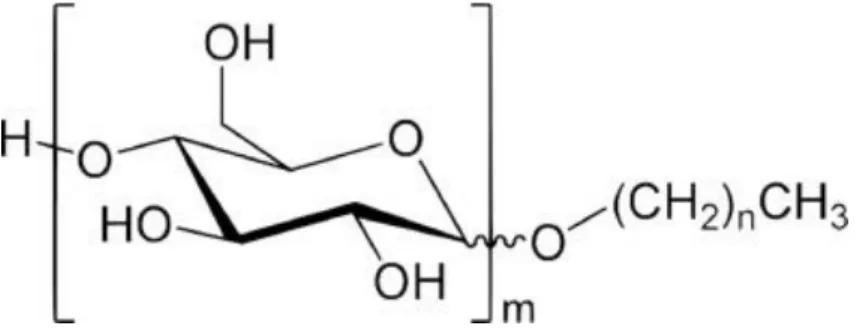
(4) 2.1.1. Experimental factors In the current study, the ST of the in vitro fermentation liquid and SSA of the substrate were considered as experimental factors. The ST of fermentation liquid was accomplished by providing the exogenous non-ionic surfactant, alkyl polyglucoside (APG general chemical structure presented in Fig. 1). APG is a strong surfactant with a ST of 28.7 dynes/cm, whereas the ST of water is 71.97 dynes/cm at 25 °C. Meanwhile, the ST of rumen buffer solution was 53.96 dynes/cm. Thus, the various gradients of ST were obtained by adding different dosages of APG. ST was changed with the concentration of APG in a format of minus exponent, and the addition of 0.12% APG (v/v) reached the lowest ST value. Therefore, by adding 0, 0.02, 0.05 and 0.12% APG, four gradients of ST values were obtained: 53.95, 46.09, 42.78, and 36.07 dynes/cm, and presented as ST1, ST2, ST3 and ST4, respectively.. Fig. 1. The general chemical structure of alkyl polyglucoside (APG).. Neutral detergent fibre (NDF) extracted from rice straw was used as a fermentation substrate material. SSA of NDF was the second experimental factor. NDF with three different particle sizes was obtained using a grinder with three screen sizes (0.15, 0.25 and 0.84 mm). These particle sizes were used to represent the known digested particle distribution in the rumen of goat (Li and Jiang, 2001 and Zhen and Ma, 1998). The SSA of the particles was determined by a Surface Area Analyzer (Quadrasorb-SI, Quantachrome Inc. Florida, CA, USA). Finally, NDF was obtained with different SSA values of 3.37, 3.73, and 4.44 cm2/g, represented as SSA1, SSA2, and SSA3, respectively.. 2.1.2. Cell surface hydrophobicity assay In the present work, the number of cell suspension for each fermentation bottle was varied from 1.0 × 109 to 2.6 × 1010 per mL, depending on the fermentation time. This is in agreement with the aim of the current study about the changes in the hydrophobicity of all microbes at different fermentation time points. The CSH of rumen mixed microbes was assessed as described in two previous works (Li and McLandsborough, 1999 and Sweet, MacFarlane and Samaranayake, 1987), using the microbial adhesion to hydrocarbon assay (MATH) (Rosenberg, Gutnick and Rosenberg, 1980 and Yang et al., 2010). Briefly, 2 mL of fermenting liquid from each bottle (216 samples = 4 ST × 3 SSA × 6 point-in-time × 3 replicates) were centrifuged (10,000 × g, 4 °C for 10 min) to obtain pellets from rumen mixed microbes. Then, the microbial pellets were washed twice and resuspended in 6 mL of 0.1 M KNO3 phosphate-buffered saline solution (pH 6.6). A high salt buffer solution was used to minimise the electrostatic effects for the determination of CSH. The resuspended solution containing the microbial pellet was homogenised by vortex oscillation for 2 min, and 2 mL of suspension was used for the optical density (OD400) measurement using an ultraviolet spectrophotometer (recorded as A 0). Next, 2 mL of hexadecane were added to new tubes containing 2 mL of suspension, followed by 2 min of homogenisation and, finally, they were equilibrated at room temperature for 10 min. After the mixture was.

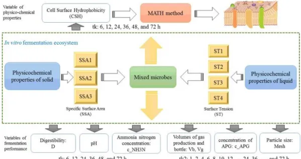
(5) completely separated into two phases, 2 mL of the lower aqueous phase were carefully collected and measured for the OD400 (recorded as A1). The hydrophobicity was calculated as follows: CSH(%) = 100 ×. A 0 − A1 A0. (1). CSH is defined as the difference between the percentage of cells retained by the hydrocarbon and aqueous layers. A0 represents the absorbance of the OD value at 400 nm before the addition of hexadecane, and A1 represents the absorbance of the OD value at 400 nm after the addition of hexadecane. 2.2. Experimental data The current CSH experimental values obtained for the first time and the data obtained in one of our previous works (Liu et al., 2013) were used as an integrated dataset to develop a predictive model. Common fermentation variables, such as pH, digestibility (D) of NDF, concentration of ammonia nitrogen (c_NH3N) and gas production (Vg) under the same experimental conditions (the combinations of 4 ST × 3 SSA) were collected from two time scale series (tk and tk2). For the CSH, D, pH, and c_NH3N variables, the time series (CSH sampling) were tk = 6, 12, 24, 36, 48, and 72 h of fermentation. For the variables of Vg, volume of bottle used for gas production (Vb), particle size (Mesh) and the concentration of APG (c_APG), the time series (Vg sampling) was tk2 = 0, 1, 2, 3, 4, 6, 8, 10, 12, 16, 24, 30, 32, 34, 36, 38, 40, 48, 54, 58, 62, and 72 h of fermentation. The data resource flowchart of the experimental section is shown in Fig. 2. Thus, the initial dataset features are SSA, ST, tk/tk2, D, c_NH3N, pH, Mesh, c_APG, Vb, and Vg.. Fig. 2. Flowchart of the experimental section used to construct the dataset..

(6) 2.3. Modelling dataset The experiment considered 12 initial levels (4 ST × 3 SSA) of environmental conditions for all experimental variables. The time series were composed by different point-in-time and time scales, such as tk: 6–72 h and tk2: 0–72 h of fermentation. In order to study non-linear effects of perturbations over CSH, the input dataset was assembled in such a way to form a combination of different variables measured in two different time series. A dataset with two blocks depending on two time series (tk and tk2) was constructed in a set of random cases (170,707 cases, without duplicate). This dataset included almost all perturbation cases of 171,072 = 216 n1 × 792 n2 (n1 = the experimental cases in the time series tk; n2 = those in the time series tk2). 2.4. EMMA-ML models In the present work, a predictive model was developed for the CSH values of ruminal microbiome as a function of perturbations of input experimental variables such as pH, c_NH3N, Vg and D. In the next step, some input terms were incorporated to measure deviations of data from the expected values (data dispersion). Thus, some variables such as V q(tk) and V'q(tk2) were defined, where the subscript q or ‘q indicated the different types of input variables, tk or tk2 (the input variables in the corresponding time scales). Furthermore, 〈CSH〉 and dVq(tk) were introduced. 〈CSH〉 represents the expected (average) values of CSH, formed by the expected measurement (EM) components used to account for the total expected value. dV q(tk) represents the Box-Jenkins Operators / perturbations (see Eq. (2)), the components used to account for the variable dispersion. Similarly, 〈Vq(tk)〉 represents the moving average of the variable “q” according to the experimental conditions (Gonzalez-Diaz et al., 2013). For each variable, such as pH, c_NH3N, Vg or D, its average value was calculated according to the different experimental conditions (conditions of ST × SSA). For instance, the moving average of 〈pH〉 included the average values under the conditions of ST1 × SSA1, ST1 × SSA2 … ST4 × SSA3. For other input variables, the moving average was also calculated according to the different conditions. dVq (tk) = Vq (tk) − 〈Vq (tk)〉. (2). These terms were added as corrections to the EM of cell surface hydrophobicity, 〈CSH〉. For Eq. (3) and the model dataset, the notation of eCSH was employed for 〈CSH〉 (expected measurement). The coefficient a1 refers to the weighted value of the expected measurement 〈 CSH〉. Therefore, the new model combined Perturbation Theory, Box-Jenkins Operators, and Time Series Analysis (Fisher, 1936). The general formula of the model proposed is presented below: CSHpred = a 0 + a1 · 𝑒CSH. (3). q=qmax ′ q=. + ∑ bq · dVq (tk) +. ′q. max. ∑. b. ′q. · dV. ′q. (tk2). ′ q=1. q=1. CSHpred represents the predicted values of CSH using the model. The subscript “q” represents the variables in the time series of tk: D, pH, and c_NH3N. The subscript “'q” represents the variables in the time series of tk2: Vb, Vg, Mesh, and c_APG. Therefore, the coefficients “bq” and “b'q” in Eq. (3) represent the weighted values of the corresponding input variables. Thus, 170,707 cases and 12 features (pool) defined the final dataset: eCSH, dSSA, dST, dtk, dD, dc_NH3N, dpH, dtk2, dMesh, dc_APG, dVb, and dVg..

(7) Seven state-of-the-art regression methods were tested: Multiple Linear regression (LM), Generalized Linear Model with Stepwise Feature Selection (GLM) (Hocking , 1976), Partial Least Squares Regression (PLS) (Wold, Ruhe, Wold, & Dunn, 1984), Lasso regression (Lasso) (R., 1994), Elastic Net regression (ENET) (H. & T., 2005), Neural Networks regression (NN) (Bishop, 1995), and Random Forest (RF) (Breiman, 2001). The simplest method is LM. The variable selection could improve the regression models and, therefore, GLM selects variables by minimizing Akaike information criterion (AIC) score (Akaike, 1974). Lasso and ENET select features via an embedded minimisation process. PLS is a coefficient optimisation algorithm directed to high variance and high correlation paths. The next methods are Machine Learning algorithms: NN and RF. NN represents a network of connected artificial neurons (simple processing units similar to the real neurons) which is able to generate precise regressions/classifications even if data are complex or incomplete. RF is a decision tree-based bagging method using a random subspace method. We run our experiments in R (Team, 2016) and we enhanced the models using the Caret Package (Kuhn et al., 2016) in order to find the best parameters automatically by repeating 10 times a 10-fold experiment for each freedom degree using a grid approach. The workflow of theoretical section for the development of EMMA-ML models could be summarised in Fig. 3: (1) Collection of the experimental data (initial dataset): tk/tk2, c_NH3N, D, pH, Mesh, c_APG, Vb, Vg; (2) Application of PT, MA, Time series to obtain the dataset, with the output variable as observed CSH and 12 input features: eCSH, dtk, dc_NH3N, dD, dpH, dtk2, dMesh, dc_APG, dVb, and dVg; (3) Manual dataset split into training (75%) and test (25%) sets: https://dx.doi.org/10.6084/m9.figshare.3189352.v1. (4) Calculation of all possible regression models: LM, GLM, PLS, Lasso, ENET, NN and RF; (5) Selection of the best EMMA-ML regression model using R-squared and Root-Mean-Square Error values to predict CSH as a general function: CSHpred = f(eCSH, dSSA, dSA, dtk, dc_NH3N, dD, dpH, dtk2, dMesh, dc_APG, dVb, dVg);. Fig. 3. Flow chart of experimental and theoretical sections of the EMMA-ML model for CSH..

(8) The best regression model can be used to predict the CSH values using new in vitro fermentation conditions. The dataset was divided into two subsets: 75% of the cases as training set and 25% of the cases as test set. The training set is used to obtain the model without the participation of the test set, which is employed to validate the power of the prediction model. Thus, our models were trained using a dataset with 128,031 perturbations and 42,676 perturbations unknown for the models were maintained in order to perform a final validation/test of the models. We performed our experiments with a 10-fold cross-validation approach in order to train our models with the training data and ensure that our findings will generalize with our independent test set and to avoid problems such as overfitting. The original dataset was separated in a 75–25 proportion for the training-test process and an internal 10-fold cross-validation process was performed with the aforementioned 75% of the data (Simon, Subramanian, Li, & Menezes, 2011). Our experiments were designed with an external set of unknown perturbations in order to detect and avoid a possible selection bias (Ambroise & McLachlan, 2002) by using our Machine Learning algorithms with the remaining 25%. We have a mixture of continuous and categorical features in our dataset, so we used a number of pre-processing steps in order to scale and transform the data: taking the logarithm of the count data (or categorical) and subtracting the mean and dividing by the standard deviation (standardization) in order to scale the data and thus, all the ML methods can deal with the dataset. No highly significant differences were found in the performance results across several experiments, therefore it was decided to present the results of one run. The efficiency of the regression models was tested using R-squared (R2) and root-mean-square error (RMSE) of training and test/validation tests. R2 measures how close the data are to the fitter regression line, and RMSE accumulates the differences between the predicted and observed values of the output variable (CSH). The models used all 12 features, without any previous feature selection or data filter. We run all the experiments in our HPC cluster called BioCAI. A cluster version of the RRegrs package (Tsiliki et al., 2015a, b) was created as an open GitHub repository entitled batchRRegrs (https://github.com/cafernandezlo/batchRRegrs/).. 3. Results and discussion 3.1. Experimental cell surface hydrophobicity The average experimental values of CSH for each condition in the first time scale (tk) are presented in Table 1. The values of CSH changed with ST of the fermentation medium and SSA of the substrate materials. Generally, all conditions (ST, SSA and time) were important for the CSH experimental values. For instance, the CSH values were significantly increased (P < 0.01) with the enhancement of SSA. They were also individually influenced by the ST of the fermentation medium (P < 0.05), and the SSA × time interaction (P < 0.05). The CSH values of the rumen microbiome were decreased with fermentation time for SSA of 3.37 and 3.73 m2/g, while it increased at 24 h for SSA of 4.44 m2/g..

(9) Table 1. The experimental measurements of cell membrane hydrophobicity (CSH). Experimental condition SSA (m2/g). 3.37. 3.73. 4.44. ST (dynes/cm). CSH (%) in the time series (tk) 6h. 12 h. 24 h. 36 h. 48 h. 72 h. 53.95. 28.6. 12.3. 13.3. 32.1. 4.1. 14.7. 46.09. 30.3. 20.5. 14.1. 39.5. 4.3. 13.1. 42.78. 32.9. 19.5. 14.6. 32.2. 8.6. 16.5. 36.07. 29.1. 14.6. 10.5. 30.7. 4.5. 17.8. 53.95. 25.9. 20.5. 13.0. 27.8. 13.2. 16.6. 46.09. 31.0. 14.1. 15.8. 18.3. 12.6. 22.0. 42.78. 31.7. 19.8. 14.1. 13.2. 4.3. 15.3. 36.07. 28.7. 20.1. 19.8. 28.5. 9.3. 20.0. 53.95. 33.0. 12.3. 17.2. 32.2. 4.9. 22.5. 46.09. 33.8. 22.1. 17.3. 35.8. 4.9. 24.0. 42.78. 34.5. 18.5. 23.5. 32.9. 7.4. 26.0. 36.07. 29.4. 24.2. 30.5. 35.9. 7.9. 33.2. The cell adhesion of rumen bacteria to a substrate is the prerequisite for microbial colonisation and proliferation. The CSH of microbes is considered an important factor during the adhesion of microorganisms to material surfaces (Ascencio, Johansson and Wadström, 1995, Balazs et al., 2003, Katsikogianni and Missirlis, 2004 and Marshall and Cruickshank, 1973), and the strains with higher hydrophobicity have stronger adhesive capability (Moser and Schröder, 1997, Nguyen, Turner and Dykes, 2011 and Pan, Li and Liu, 2006). Our results showed that the CSH of microbes was enhanced with the increase of SSA, and it was higher in the initial fermentation stage than in the later stage. This suggested that the higher substrate values of SSA could positively enhance the microbial CSH, and further increase the adhesion of bacteria to forage. It also implied that the adherence of bacteria to substrate could be changed with the fermentation time. As the previous research studies have proven, the surface hydrophobicity property of bacteria depends on the material composition and cell physiological components, such as the cell surface protein (Parker & Munn, 1984), polysaccharides (Devasia, 1993), phospholipids (Rosenberg, 1991), capsule and slime layer (Hogt, 1983). Baselga et al. (1992) observed that the hydrophobicity of ruminant mastitis Staphylococcus aureus can be increased during the logarithmic growth phase, and freshly isolated strains are more hydrophobic than old strains. Zhang et al. (2010) also reported that the surface hydrophobicity of a Serratia spp. strain decreased with time after the logarithmic phase during fermentative growth. 3.2. EMMA-ML models This work proposed a general predictive model for CSH based on the data of the current study under the conditions of ST and SSA and data reported in our previous work (Liu et al., 2013). The scientists are always looking for connections between different experimental systems and theoretical studies in order to replace the traditional partial researches with the macroscopic view of the integral ecosystems, obtaining new rules and knowledge. However, combining diverse experimental conditions into an integral ecosystem is an issue that every scientist has to overcome. Table 2 summarises the definition of all the applied features of cell surface hydrophobicity..

(10) Table 2. Dataset features for the prediction models of cell surface hydrophobicity (CSH). Feature notation. Feature description. Feature notation. Feature description. eCSH. Expected cell surface hydrophobicity as the dpH average of experimental CSH by the experimental conditions. Moving average of pH. dSSA. Moving average of specific surface area. dtk2. Moving average of the second time scale. dST. Moving average of suspending liquid surface tension. dMesh. Moving average of particle size. dtk. Moving average of the first time scale. dc_APG. Moving average of the concentration of alkyl polyglucoside (exogenous non-ionic surfactant). dD. Moving average of neutral detergent fibre digestibility. dVb. Moving average of the volume of bottle used for gas production. dc_NH3N. Moving average of ammonia – nitrogen concentration. dVg. Moving average of gas production. Thus, the use of PT, MA, and ML was proposed in order to develop theoretical models to reduce the deviations or variations of different conditions on the experimental values of input parameters in the situation of dual-time scales. Our attempt was to develop for the first time a unified EMMAML model that was able to merge all these properties, such as CSH and parameters/variables of fermentation performance. The EMMA-ML model developed herein was able to directly predict the output properties of CSH after perturbations under the experimental conditions. The results for seven ML regression methods are presented in Table 3: LM, GLM, PLS, LASSO, ENET, NN, and RF. The values of R2 and RMSE for test/validation set were used to choose the best CSH prediction model. The parameters and function name for each method are presented in Table 4. All the regression methods used the same default settings, such as 10-fold cross-validation, 10 repeats and RMSE metrics. The full code sources and example inputs and outputs can be downloaded from the open GitHub repository entitled batchRRegrs (https://github.com/cafernandezlo/batchRRegrs/)..

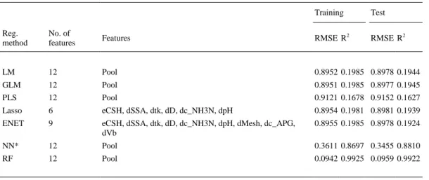
(11) Table 3. EMMA-ML models. Training. Test RMSE R2. Reg. method. No. of features. Features. RMSE R2. LM. 12. Pool. 0.8952 0.1985 0.8978 0.1944. GLM. 12. Pool. 0.8951 0.1985 0.8977 0.1945. PLS. 12. Pool. 0.9121 0.1678 0.9152 0.1627. Lasso. 6. eCSH, dSSA, dtk, dD, dc_NH3N, dpH. 0.8954 0.1981 0.8981 0.1939. ENET. 9. eCSH, dSSA, dtk, dD, dc_NH3N, dpH, dMesh, dc_APG, dVb. 0.8955 0.1985 0.8978 0.1924. NN*. 12. Pool. 0.3611 0.8697 0.3455 0.8810. RF. 12. Pool. 0.0942 0.9925 0.0959 0.9922. Note: R2 = R-squared, RMSE = Root-mean-square error, LM = Multiple linear regression, GLM = Generalized linear model with stepwise feature selection, PLS = Partial least squares regression, LASSO = Lasso regression, ENET = Elastic net regression, NN = Neural network, RF = Random Forest; Pool = eCSH, dSSA, dST, dtk, dD, dc_NH3N, dpH, dtk2, dMesh, dc_APG, dVb, dVg.

(12) Table 4. Parameters for the regression function in batchRRegrs. Regression Method. Regression function in batchRRegrs. Parameters. LM. LMreg. Tuning parameters:. GLM. GLMreg. Using package MASS with no tuning parameters. PLS. PLSreg. Using package pls with tuning parameters:. Intercept (intercept, logical). Number of components (ncomp, numeric) Code: floor.param<-floor((dim(my.data.train)[2]-1)/5) if(floor.param<1){floor.param <- 1} tuneGrid = expand.grid(.ncomp = c(1:floor.param))) Lasso. LASSOreg. Using package elasticnet with tuning parameters: Fraction of full solution (fraction, numeric) Code: tuneGrid = expand.grid(.fraction = seq(0.1,1,by= 0.1)). ENET. ENETreg. Using package glmnet with tuning parameters: Mixing percentage (alpha, numeric) Regularization parameter (lambda, numeric) Code: tuneGrid = expand.grid(.alpha = seq(0.1,1,length = 10), .lambda = 99). NN. NNreg. MaxNWts = 20,000 Using package nnet with tuning parameters: Number of hidden units (size, numeric) Weight decay (decay, numeric) Code: tuneGrid = expand.grid(.size = c(200,300,400),.decay = c(0,0.01,0.2,0.1))). RF. RFreg. ntree = 50 Using package randomForest with tuning parameters: Number of randomly selected predictors (mtry, numeric) Code:tuneParam = data.frame(.mtry = c(2:12)).

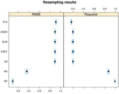
(13) The difference in quantitative terms using RMSE and R2 during the cross-validation process for all the regression methods is shown in Fig. 4. The plot demonstrates that all the methods are stable.. Fig. 4. Boxplot showing the stability of the regression methods during the 10fold cross-validation process.. In addition, the results showed that the simple methods LM, GM, PLS, Lasso and ENET provided poor models with R2 < 0.20 for both training and test series. For NN, the addition of artificial neurons in the hidden layer was explored (with different values for the weight decay of the neural net) in order to improve the results (see Fig. 5). We found that increasing the number of elements in the hidden layer over 200 just increase the error rate. Thus, this parameter is the performance limit for this method. Finally, the R2 of 0.88 was obtained with the test dataset.. Fig. 5. (a) RMSE and (b) R-squared (R2) performance of NN according to the number of artificial neurons in the hidden layer..

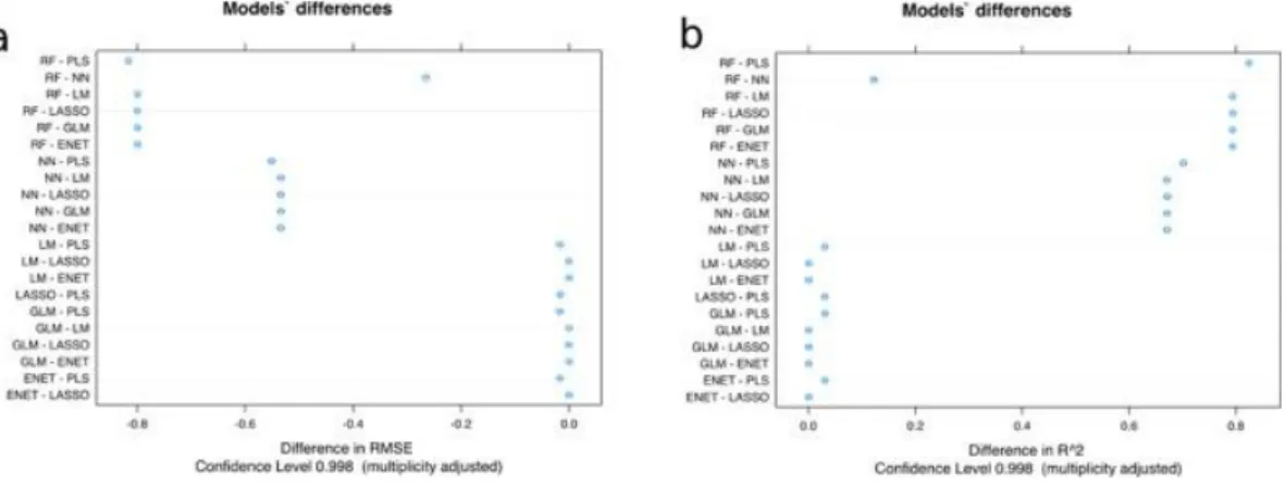
(14) Only Lasso and ENET were able to reduce the number of features to 6 and, respectively, 9, with similar performance as LM and GLM using 12 features. PLS obtained the worst performance, with R2 of 0.16. The differences between the models are presented in Fig. 6.. Fig. 6. Differences of the models obtained using the RMSE and R 2 of all pairwise model comparisons: average performance value (dot) with two-sided confidence limits computed by Student t-test with Bonferroni multiplicity correction.. The RF model is based on the original implementation of the Random Forest algorithm by Breiman (2001), widely used in ML. This method generates multiple bootstrapped versions of the data and fits a decision tree for each data subset. In the end, the RF uses each decision tree in order to give the final solution to the problem. This particular ML model is known to perform very well with high-dimensional datasets, avoiding overfitting due to its particular characteristic, allowing an averaging effect across all the single models (Chen & Ishwaran, 2012). A number of trees were built based on bootstrapped samples (for training), where a random sample of predictors (features) is chosen as the candidates from the full set of features p of the dataset. Each time, a fresh set of features was taken into account, thus the algorithm is not allowed to consider most of the available features, only a square root of the total number of predictors in classification and p/3 in regression. As shown in Fig. 7(a), the fitted versus observed plot of the best model (in red) was very close to the expected regressed diagonal line (in blue). Fig. 7(b) shows that the best number of trees for the RF, in order to avoid overfitting was 50 trees with 6 randomly selected parameters according to the R2 results as it reached the plateau. During the 10-fold cross validation process, the results shown in Fig. 7(c) were obtained. Furthermore, Fig 7(d) shows that three of the features are more important for the model: dtk, dD and dc_NH3N. This was calculated using IncNodePurity, a measure of the decrease of the impurity in the nodes from different bootstrapped splits, averaged over all trees. Therefore, it can be observed that the variation of the first time scale dtk is very important for the model. The neutral detergent fibre digestibility (dD) influences the cell surface properties, and the ammonia-nitrogen concentration (dc_NH3N) is also important for the CSH, which has similarly been proven in previous works ( Liu et al., 2013)..

(15) Fig. 7. (a) The fitted versus observed plot, (b) the R-squared results according to the number of trees, (c) the results during the 10-fold cross-validation process, and finally, (d) the importance of each feature for the best model EMMA-RF. (For interpretation of the references to colour in this figure legend, the reader is referred to the web version of this article.). Several experimental runs were performed to find the best combination of number of trees and randomly selected parameters in order to avoid overfitting. It was found that 50 trees was the optimum amount (Biau, 2012 ; Mayumi Oshiro, Santoro Perez and Augusto Baranauskas, 2012) with 6 randomly selected parameters. In general, the more trees one used, the better the results. However, in the case of our dataset, the regression improvement decreased as the number of trees increased. Thus, at a certain point, the benefit in prediction performance from learning more trees was lower than the cost in computation time for learning these additional trees. In addition, a trend of overfitting in the model was also observed, although it seemed that most of the times was not significant (Breiman, 2001). The code in R of the RF regression function is described below:.

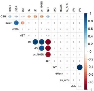
(16) RFreg < function(my.datf.train,my.datf.test, sCV,iSplit=1,fDet=F,outFile="") { #=============================== # Basic RandomForest #=============================== # make available the names of variables from training dataset net.c = my.datf.train[,1] RegrMethod <- "rf" # type of regression # Define the CV conditions ctrl<- trainControl(method=sCV,number=10, repeats=10,summaryFunction=defaultSummary) tuneParam = data.frame(.mtry=c(2:12)) # Train the model using only training set rf.fit<- train(net.c∼.,data=my.datf.train, method=′rf′,trControl=ctrl, metric=′RMSE′,ntree=50,tuneGrid=tuneParam) … } The full code sources and example inputs and outputs can be downloaded from the open Github repository entitled batchRRegrs (the cluster version of RRegrs (Tsiliki et al., 2015b), https://github.com/cafernandezlo/batchRRegrs/).. An additional study of the positive and negative correlation between all the features/output variables for the current dataset (training and test) is presented in Fig. 8. It should be pointed out that the ruminal in vitro gas production (dVg) is not strongly related to the expected CSH values of ruminal mixed microbes. The positive correlation between dtk and dD, dc_NH3N is a natural consequence of the fermentation process. In addition, the positive correlation between digestibility (dD) and dc_NH3N should also be emphasised, along with the negative correlation between dpH and dD, dC_NH3N. The positive correlation between dVg and dtk2 is explained by the fact that in time the gas production increases. The plot shows that there are no significant correlations between the observed CSH values and the features of the model, demonstrating the lack of a linear prediction model for this dataset..

(17) Fig. 8. Correlations between dataset features/CSH observed values (CSH) obtained with corrplot package from R.. Breiman stated that RF did not overfit, so it could be said that one can use as many trees as they want, taking into consideration only the size of the dataset and the computational costs of the experiments. However, Segal (2004) found that RF overfitted for some noisy datasets, especially in regression. The best EMMA-ML model was obtained using the most complex method, RF (EMMA-RF). The model is based on all 12 features and it is characterised by R2 and RMSE values of 0.99 and 0.09, respectively, for test set (on a dataset > 170 000 perturbation cases). The optimised model for the CSH prediction is able to predict the effects of perturbations under the experimental conditions or variables Vq(tk) over CSH of ruminal microbes. It showed that both time series (tk and tk2) contributed to the prediction of CSH with the RF model.. 4. Conclusions The current work presented for the first time an EMMA-ML model to forecast the CSH values, a Perturbation Theory model that used the Expected Measure (EM) of CSH as input variables combined with the theory of Box-Jenkins Operators and Time Series Analysis. Perturbations were used in all input variables (SSA, ST, pH, c_NH3N, D, Vb, and Vg) in dual-time series with various scales. The best CSH prediction model used the RF method (EMMA-RF) and it was based on 12 input variables, with the test R2 of 0.992. On the one hand we found that simple models such as LM, GLM, PLS, Lasso and ENET are unable to deal with a huge dataset like the one proposed in this paper. On the other hand, we found that complex, state-of-the-art NN and RF, a well-known powerful nonparametric statistical method, considers this dataset enough informative to learn the inherent complexity of the data in terms of number of cases..

(18) The objective of the current work was to develop a model able to rationalise and predict the effect of all the input variables, such as SSA, ST, pH, fibre digestibility, etc. over the cell surface hydrophobicity of the microbiome by using samples of mix microbiome (bacteria and protozoa together). A future direction of our research could be the differentiation of the effect on different types of cells, such as positive gut bacteria, pathogen bacteria, pathogen protozoa, etc. under different feeding treatments. This could open new ways of improving feeding quality for animals. The model demonstrated the increased importance of the in vitro fermentation parameters such as CSH expected value (eCSH), digestibility (dD) and ammonia – nitrogen concentration (dc_NH3N) for the prediction of the cell surface hydrophobicity.. Acknowledgments The authors would like to thank for the grants from the National Natural Science Foundation of China (Grant No. 31172234, and No. 31260556), the Planned Science and Technology Project of Hunan Province (2015NK3041), ``Strategic Priority Research Program - Climate Change: Carbon Budget and Relevant Issues'' of the Chinese Academy of Science (Grant No. XDA05020700) and Hunan Provincial Creation Development Project (Grant No. 2013TF3006). The authors gratefully acknowledge the support from the Key Laboratory of Subtropical Agro-ecological Engineering, Institute of Subtropical Agriculture, and the Chinese Academy of Sciences (CAS) for providing all the experimental materials and apparatus. The authors would also like to thank Tao Ran for the assistance in reviewing the manuscript. This project was also supported by the General Directorate of Culture, Education and University Management of Xunta de Galicia (Ref. GRC2014/049), Spain and finally by the Spanish Ministry of Economy and Competitiveness for its support with the funding of the unique installation BIOCAI (UNLC08-1E-002, UNLC13-13-3503) and the European Regional Development Funds (FEDER) by the European Union and the “Juan de la Cierva” fellowship program supported by the Spanish Ministry of Economy and Competitiveness (Carlos Fernandez-Lozano, Ref. FJCI-2015-26071). The authors declare that there are no conflicts of interest.. References Aires-de-Sousa and Gasteiger, 2005. J. Aires-de-Sousa, J. Gasteiger. Prediction of enantiomeric excess in a combinatorial library of catalytic enantioselective reactions. Journal of Combinatorial Chemistry, 7 (2005), pp. 298–301. Akaike, 1974. H. Akaike. A new look at the statistical model identification. IEEE Transactions on Automatic Control, 19 (1974), pp. 716–723. Ambroise and McLachlan, 2002. C. Ambroise, G.J. McLachlan. Selection bias in gene extraction on the basis of microarray gene-expression data. Proceedings of the National Academy of Sciences of the United States of America, 99 (2002), pp. 6562–6566. Ascencio, Johansson and Wadström, 1995. F. Ascencio, G. Johansson, T. Wadström. Cell-surface charge and cell-surface hydrophobicity of collagen-binding aeromonas and vibrio strains. Archives of Microbiology, 164 (1995), pp. 223–230. Babu and Reddy, 2014. C.N. Babu, B.E. Reddy. A moving-average filter based hybrid ARIMA–ANN model for forecasting time series data. Applied Soft Computing, 23 (2014), pp. 27–38. Balazs et al., 2003. D.J. Balazs, K. Triandafillu, Y. Chevolot, B.O. Aronsson, H. Harms, P. Descouts, et al. Surface modification of PVC endotracheal tubes by oxygen glow discharge to reduce bacterial adhesion. Surface and Interface Analysis, 35 (2003), pp. 301–309. Barba, Rodríguez and Montt, 2014. L. Barba, N. Rodríguez, C. Montt. Smoothing strategies combined with ARIMA and neural networks to improve the forecasting of traffic accidents. The Scientific World Journal (2014), p. 12 2014. Baselga et al., 1992. R. Baselga, I. Albizu, J.R. Penadés, B. Aguilar, M. Iturralde, B. Amorena. Hydrophobicity of ruminant mastitis Staphylococcus aureus in relation to bacterial aging and slime production. Current Microbiology, 25 (1992), pp. 173–179. Biau, 2012. G. Biau. Analysis of a random forests model. Journal of Machine Learning Research, 13 (2012), pp. 1063–1095..

(19) Bishop, 1995. C.M. Bishop. Neural networks for pattern recognition. Oxford University Press (1995). Box and Jenkins, 1968. G.E.P. Box, G.M. Jenkins. Some recent advances in forecasting and control. Journal of the Royal Statistical Society. Series C (Applied Statistics), 17 (1968), pp. 91–109. Breiman, 2001. L. Breiman. Random Forests. Machine Learning, 45 (2001), pp. 5–32. Brown and Jaffé, 2006. D.G. Brown, P.R. Jaffé. Effects of nonionic surfactants on the cell surface hydrophobicity and apparent hamaker constant of a sphingomonas sp. Environmental Science & Technology, 40 (2006), pp. 195–201. Chen and Ishwaran, 2012. X. Chen, H. Ishwaran. Random Forest for genomic data analisis. Genomics, 99 (2012), pp. 323–329. Christensen et al., 1985. G.D. Christensen, W.A. Simpson, J.J. Younger, L.M. Baddour, F.F. Barrett, D.M. Melton, et al. Adherence of coagulase-negative staphylococci to plastic tissue culture plates: A quantitative model for the adherence of staphylococci to medical devices. Journal of Clinical Microbiology, 22 (1985), pp. 996–1006. Devasia, 1993. P. Devasia. Surface chemistry of Thiobacillus ferrooxidans relevant to adhesion on mineral surfaces. Applied and Environmental Microbiology, 59 (1993), pp. 4051–4055. Drumm, Neumann, Policova and Sherman, 1989. B. Drumm, A.W. Neumann, Z. Policova, P.M. Sherman. Bacterial cell surface hydrophobicity properties in the mediation of in vitro adhesion by the rabbit enteric pathogen Escherichia coli strain RDEC-1. Journal of Clinical Investigation, 84 (1989), pp. 1588–1594. Fisher, 1936. R.A. Fisher. The use of multiple measurements in taxonomic problems. Annals of Eugenics, 7 (1936), pp. 179–188. Gallardo-Moreno et al., 2002. A.M. Gallardo-Moreno, A. Méndez-Vilas, M.L. González-Martín, M.J. Nuevo, J.M. Bruque, E. Garduño, et al. Comparative study of the hydrophobicity of Candida parapsilosis 294 through macroscopic and microscopic analysis. Langmuir, 18 (2002), pp. 3639–3644. Gonzalez-Diaz et al., 2013. H. Gonzalez-Diaz, S. Arrasate, A. Gomez-SanJuan, N. Sotomayor, E. Lete, L. Besada-Porto, et al. General theory for multiple input-output perturbations in complex molecular systems. 1. Linear QSPR electronegativity models in physical, organic, and medicinal chemistry. Current Topics in Medicinal Chemistry, 13 (2013), pp. 1713–1741. H. and T., 2005. Z. H., H. T.. Regularization and variable selection via the elastic net. Journal of the Royal Statistical Society Series B Statistical Methodology, 67 (2005), pp. 301–320. Hocking, 1976. R.R. Hocking. The analysis and selection of variables in linear regression. Biometrics, 32 (1976), pp. 1–49. Hogt, 1983. A.H. Hogt. Adhesion of coagulase-negative staphylococci to biomaterials. FEMS Microbiology Letters, 18 (1983), pp. 211–215. Katsikogianni and Missirlis, 2004. M. Katsikogianni, Y.F. Missirlis. Concise review of mechanisms of bacterial adhesion to biomaterials and of techniques used in estimating bacteria-material interactions. European Cells and Materials, 8 (2004), pp. 37–57. Kleandrova et al., 2014. V.V. Kleandrova, F. Luan, H. Gonzalez-Diaz, J.M. Ruso, A. Melo, A. SpeckPlanche, et al. Computational ecotoxicology: Simultaneous prediction of ecotoxic effects of nanoparticles under different experimental conditions. Environment International, 73 (2014), pp. 288–294. Kuhn et al., 2016. M. Kuhn, Contributions from Jed Wing, S. Weston, A. Williams, C. Keefer, A. Engelhardt, et al. caret: classification and regression Training. R package version 6.0-68. (2016). https://CRAN.Rproject.org/package=caret.. Leontiadou, Mark and Marrink, 2004. H. Leontiadou, A.E. Mark, S.J. Marrink. Molecular dynamics simulations of hydrophilic pores in lipid bilayers. Biophysical Journal, 86 (2004), pp. 2156–2164. Li and Jiang, 2001. J.S. Li, Z.W. Jiang. Distribution of food particles with different size in the digestive tract in Mongolian gazelle. Acta Zoologica Sinica, 47 (2001), pp. 488–494. Li and McLandsborough, 1999. J. Li, L.A. McLandsborough. The effects of the surface charge and hydrophobicity of Escherichia coli on its adhesion to beef muscle. International Journal of Food Microbiology, 53 (1999), pp. 185–193. Li et al., 2011. X. Li, L. Petersen, S. Broderick, B. Narasimhan, K. Rajan. Identifying factors controlling protein release from combinatorial biomaterial libraries via hybrid data mining methods. ACS Combinatorial Science, 13 (2011), pp. 50–58. Liu et al., 2015. Y. Liu, G. Buendia-Rodriguez, C.G. Penuelas-Rivas, Z. Tan, M. Rivas-Guevara, E. TenorioBorroto, et al. Experimental and computational studies of fatty acid distribution networks. Molecular BioSystems, 11 (2015), pp. 2964–2977. Liu et al., 2016. Y. Liu, C.G. Peñuelas-Rivas, E. Tenorio-Borroto, M. Rivas-Guevara, G. Buendía-Rodríguez, Z. Tan, et al. Chemometric approach to fatty acid metabolism-distribution networks and methane production in ruminal microbiome. Chemometrics and Intelligent Laboratory Systems, 151 (2016), pp. 1– 8. Liu et al., 2013. Y. Liu, T. Ran, Z-l. Tan, S-x. Tang, P-p. Wang. Effects of surface tension and specific surface areas on in vitro fermentation of fiber. Acta Veterinaria et Zootechnica Sinica, 44 (2013), pp. 901–910 (in Chinese)..

(20) Liu et al., 2016. Y. Liu, T. Ran, E. Tenorio-Borroto, S. Tang, A. Pazo, Z. Tan, et al. Experimental and chemometric studies of cell membrane permeability. Chemometrics and Intelligent Laboratory Systems, 154 (2016), pp. 1–6. Marshall and Cruickshank, 1973. K.C. Marshall, R.H. Cruickshank. Cell surface hydrophobicity and the orientation of certain bacteria at interfaces. Archives of Microbiology, 91 (1973), pp. 29–40. Mayumi Oshiro, Santoro Perez and Augusto Baranauskas, 2012. T. Mayumi Oshiro, P. Santoro Perez, J. Augusto Baranauskas. How many trees in a random forest?. P. Perner (Ed.), 8th international conference on machine learning and data mining in pattern recognition (MLDM'12), Springer-Verlag, Berlin, Heidelberg (2012), pp. 154–168. Messina, Besada-Porto, González-Díaz and Ruso, 2015. P.V. Messina, J.M. Besada-Porto, H. González-Díaz, J.M. Ruso. Self-assembled binary nanoscale systems: multioutput model with LFER-covariance perturbation theory and an experimental–computational study of NaGDC-DDAB Micelles. Langmuir (2015). Moser and Schröder, 1997. I. Moser, W. Schröder. Hydrophobic characterization of thermophilic Campylobacter species and adhesion to INT 407 cell and fibronectin. Microbial Pathogenesis, 22 (1997), pp. 155–164. Nguyen, Turner and Dykes, 2011. V.T. Nguyen, M.S. Turner, G.A. Dykes. Influence of cell surface hydrophobicity on attachment of Campylobacter to abiotic surfaces. Food Microbiology, 28 (2011), pp. 942–950. Oskoui et al., 2013. S.A. Oskoui, A. Niaei, H.-H. Tseng, D. Salari, B. Izadkhah, S.A. Hosseini. Modeling preparation condition and composition–activity relationship of perovskite-type LaxSr1–xFeyCo1–yO3 nano catalyst. ACS Combinatorial Science, 15 (2013), pp. 609–621. Pan, Li and Liu, 2006. W.H. Pan, P.L. Li, Z.Y. Liu. The correlation between surface hydrophobicity and adherencevof Bifidobacterium strains from centenarians' faeces. Anaerobe, 12 (2006), pp. 148–152. Parker and Munn, 1984. N.D. Parker, C.B. Munn. Increased cell surface hydrophobicity associated with possession of an additional surface protein by Aeromonas salmonicida. FEMS Microbiology Letters, 21 (1984), pp. 233–237. Rosenberg, 1991. M. Rosenberg. Basic and applied aspects of microbial adhesion at the hydrocarbon: Water interface. Critical Reviews in Microbiology, 18 (1991), p. 159. Rosenberg, Gutnick and Rosenberg, 1980. M. Rosenberg, D. Gutnick, E. Rosenberg. Adherence of bacteria to hydrocarbons: A simple method for measuring cell-surface hydrophobicity. FEMS Microbiology Letters, 9 (1980), pp. 29–33. Segal, 2004. M.R. Segal. Machine learning benchmarks and random forest regression. Center for bioinformatics & molecular biostatistics, Center for Bioinformatics and Molecular Biostatistics, UC San Francisco (2004). Shida et al., 2013. T. Shida, H. Koseki, I. Yoda, H. Horiuchi, H. Sakoda, M. Osaki. Adherence ability of Staphylococcus epidermidis on prosthetic biomaterials: An in vitro study. International Journal of Nanomedicine, 8 (2013), pp. 3955–3961. Simon, Subramanian, Li and Menezes, 2011. R.M. Simon, J. Subramanian, M.C. Li, S. Menezes. Using cross-validation to evaluate predictive accuracy of survival risk classifiers based on high-dimensional data. Briefings in Bioinformatics, 12 (2011), pp. 203–214. Su and Yan, 2010. G. Su, B. Yan. Nano-combinatorial chemistry strategy for nanotechnology research. Journal of Combinatorial Chemistry, 12 (2010), pp. 215–221. Sweet, MacFarlane and Samaranayake, 1987. S.P. Sweet, T.W. MacFarlane, L.P. Samaranayake. Determination of the cell surface hydrophobicity of oral bacteria using a modified hydrocarbon adherence method. FEMS Microbiology Letters, 48 (1987), pp. 159–163. Team, 2016. R.D.C. Team. R: A language and environment for statistical computing. R Foundation for Statistical Computing, Vienna, Austria (2016). Tibshirani, 1994. R. Tibshirani. Regression selection and shrinkage via the lasso. Journal of the Royal Statatistical Society: Series B Statistical Methodoogyl, 58 (1994), pp. 267–288. Tsiliki et al., 2015b. G. Tsiliki, C.R. Munteanu, J.A. Seoane, C. Fernandez-Lozano, H. Sarimveis, E.L. Willighagen. RRegrs: An R package for computer-aided model selection with multiple regression models. Journal of Cheminformatics, 7 (2015), p. 46. Tsiliki et al., 2015a. G. Tsiliki, C.R. Munteanu, J. Seoane, C. Fernandez-Lozano, H. Sarimveis, E. Willighagen. Using the RRegrs R package for automating predictive modelling. MOL2NET - sciforum electronic conference seriesVol. 1 (2015), p. F009. Turias, González, Martin and Galindo, 2008. I. Turias, F. González, M.L. Martin, P. Galindo. Prediction models of CO, SPM and SO2 concentrations in the Campo de Gibraltar Region, Spain: A multiple comparison strategy. Environmental Monitoring and Assessment, 143 (2008), pp. 131–146. Ukuku and Fett, 2002. D.O. Ukuku, W.F. Fett. Relationship of cell surface charge and hydrophobicity to strength of attachment of bacteria to cantaloupe rind. Journal of Food Protection, 65 (2002), pp. 1093– 1099..

(21) Wold, Ruhe, Wold and Dunn, 1984. S. Wold, A. Ruhe, H. Wold, W.J. Dunn III. The collinearity problem in linear regression. The partial least squares (PLS) approach to generalized inverses. SIAM Journal on Scientific and Statistical Computing, 5 (1984), pp. 735–743. Yang et al., 2010. Y.-F. Yang, Y. Li, Q.-L. Li, L.-S. Wan, Z.-K. Xu. Surface hydrophilization of microporous polypropylene membrane by grafting zwitterionic polymer for anti-biofouling. Journal of Membrane Science, 362 (2010). Yoda et al., 2014. I. Yoda, H. Koseki, M. Tomita, T. Shida, H. Horiuchi, H. Sakoda, et al. Effect of surface roughness of biomaterials on Staphylococcus epidermidis adhesion. BMC Microbiology, 14 (2014), p. 234. Zhang et al., 2010. C. Zhang, L. Jia, S.H. Wang, J. Qu, K. Li, L.L. Xu, et al. Biodegradation of betacypermethrin by two Serratia spp. with different cell surface hydrophobicity. Bioresource Technology, 101 (2010), pp. 3423–3429. Zhen and Ma, 1998. Y.G. Zhen, L. Ma. Comparative study on fibre digestion and rumen digestion dynamics in small ruminants fed various low-quality roughage. Journal of Jilin Agricultural University, 20 (1998), pp. 66–72. Zita and Hermansson, 1997. A. Zita, M. Hermansson. Determination of bacterial cell surface hydrophobicity of single cells in cultures and in wastewater in situ. FEMS Microbiology Letters, 152 (1997), pp. 299– 306. ..

(22)