DMR API: Improving cluster productivity by turning applications into malleable

Texto completo

(1)DMR API: Improving Cluster Productivity by Turning Applications into MalleableI Sergio Isertea,∗, Rafael Mayoa , Enrique S. Quintana-Ortı́a , Vicenç Beltranb , Antonio J. Peñab a. Universitat Jaume I (UJI), Castelló de la Plana, Spain b Barcelona Supercomputing Center (BSC). Abstract Adaptive workloads can change on–the–fly the configuration of their jobs, in terms of number of processes. To carry out these job reconfigurations, we have designed a methodology which enables a job to communicate with the resource manager and, through the runtime, to change its number of MPI ranks. The collaboration between both the workload manager—aware of the queue of jobs and the resources allocation—and the parallel runtime—able to transparently handle the processes and the program data—is crucial for our throughput-aware malleability methodology. Hence, when a job triggers a reconfiguration, the resource manager will check the cluster status and return the appropriate action: i) expand, if there are spare resources; ii) shrink, if queued jobs can be initiated; or iii) none, if no change can improve the global productivity. In this paper, we describe the internals of our framework and demonstrate how it reduces the global workload completion time along with providing a more efficient usage of the underlying resources. For this purpose, we present a thorough study of the adaptive workloads processing by showing the detailed behavior of our framework in representative experiments. Keywords: MPI Malleability, Job Reconfiguration, Dynamic Reallocation, Smart Resource Utilization, Adaptive workload I. This is an extended version of a previous work presented in the ICPP’17 workshop P2S2 [1]. ∗ Corresponding author Email addresses: siserte@uji.es (Sergio Iserte), mayo@uji.es (Rafael Mayo), quintana@uji.es (Enrique S. Quintana-Ortı́), vbeltran@bsc.es (Vicenç Beltran), antonio.pena@bsc.es (Antonio J. Peña). Preprint submitted to Parallel Computing. July 13, 2018.

(2) 1. Introduction In production HPC facilities, applications run on shared computers where hundreds or thousands of other applications are competing for the same resources. In this scenario, applications are submitted to the system with the shape of parallel jobs that conform the current workload of a system. Adapting the workload to the infrastructure can render considerable improvements in resource utilization and productivity. A potential approach to obtain the desired adaptivity consists in applying dynamic job reconfiguration, which devises resource usage to be potentially changed at execution time. Adapting the workload to the target infrastructure brings benefits to both system administrators and end users. While administrators would like to see the throughput rate increased and a smarter resource utilization by the applications, end-users are the direct beneficiaries of the dynamic reconfiguration, since it removes strict resource requirements at submission time. Although this may prevent the application from being executed in the shortest time, users generally experience a faster completion time (waiting plus execution time). In order to adapt a workload dynamically to the infrastructure, we need two main tools: (1) a resource manager system (RMS) capable of reallocating the resources assigned to a job; and (2) a parallel runtime to rescale an application. In our solution, we have connected these components by developing a communication layer between the RMS and the runtime. In this work we enhance the Slurm Workload Manager [2] to achieve fair dynamic resource assignment while maximizing the cluster throughput. We select Slurm1 because it is open-source, portable, and highly scalable. Moreover, it is one of the most widely-adopted RMSs in the Top500 List.2 To exploit a collection of distributed resources, the vast majority of the scientific applications that run on high performance clusters use the Message Passing Interface (MPI), either directly or on top of programming models or libraries leveraging MPI underneath. Reconfiguration is possible in MPI applications via the MPI spawning functionality. 1 2. http://slurm.schedmd.com http://www.top500.org. 2.

(3) The direct use of MPI to handle migrations, however, requires considerable effort from skilled software developers to manage the whole set of data transfers among processes in different communicators. For this purpose, we benefit from the recently-incorporated offload semantics of the OmpSs programming model [3] to ease the malleability and data redistribution process. In addition, we adapt the Nanos++ OmpSs runtime to interact with Slurm. We improve the Nanos++ runtime to reconfigure MPI jobs and establish a direct communication with the RMS. For that, applications will expose “reconfiguring points” where, signaled by the RMS, the runtime will assist to resize a job on–the–fly. We emphasize that, although we benefit from the OmpSs infrastructure and semantics for job reconfiguration, our proposal may well be leveraged as a specific-purpose library, and applications using this solution are free to exploit on-node parallelism using other programming models such as OpenMP. In summary, the main contribution of this paper is a mechanism to accomplish MPI malleability, based on existing components (MPI, OmpSs, and Slurm), which enhances resource usage to produce higher global throughput in terms of executed jobs per unit of time. Our solution, the dynamic management of resources (DMR) API, targets MPI applications and is implemented leveraging the OmpSs programming model. OmpSs provides an OpenMP-like syntax which does not interfere with other OpenMP directives or functions that may be used in the code. To that extent, we propose (1) an extension of the OmpSs offload mechanism to deal with dynamic reconfiguration; (2) a reconfiguration policy for the RMS to decide whether a job must be expanded or shrunk; and (3) a communication protocol for the runtime to interact with the RMS, based on application-level Application Programming Interface (API) calls. Last, (4) we also provide an extensive evaluation of the framework that demonstrates the benefits of our workload-aware approach. This article extends our previous work in [1] by providing an extensive overhead study of the scheduling and resize times for reconfiguring jobs. Furthermore, we have improved the workload execution analysis with a job– to–job comparison when these have been launched fixed and malleable. We focus our attention on how each job behaves when studying its individual waiting, executing and completing times. The rest of this paper is structured as follows: Section 2 discusses related work. Section 3 presents an overview of the proposed methodology. Sections 4 and 5 present the extensions developed in the Slurm RMS and the Nanos++ runtime that support our programming model proposal discussed 3.

(4) in Section 6. Section 7 evaluates and analyzes malleability in a production environment. Finally, Section 8 outlines the conclusions. 2. Related Work In general, a job (application) may be classified in one of the following types: rigid, moldable, malleable and evolving [4]. These classes depend on the number of concurrent processes during the execution of a job, so that we collapse them into two categories: • Fixed: The number of parallel processes remains constant during the execution (rigid and moldable applications). • Malleable: The number of processes can be reconfigured on–the–fly, allowing distinct numbers of parallel processes in different parts of the execution (malleable and evolving applications) or job malleability. This action is known as dynamic reconfiguration. The first steps toward malleability targeted shared-memory systems exploiting the malleability of applications. In [5] the authors leveraged moldability together with preemptive policies, such as equipartitioning (assignation of the same amount of resources to all the running jobs) and folding (the job with more resources releases half of them in favor of a pending job or the job with the fewest resources assigned). These policies can interrupt active jobs to redistribute processors among the pending jobs. Checkpointing mechanisms have been used in the past to save the application state and resume its execution with a different number of processes, or simply to migrate the execution to other processes. The work in [6] explores how malleability can be used in checkpoint-restart (C/R) applications. There, a checkpoint–and–reconfigure mechanism is leveraged to restart applications with a different number of processes from data stored in checkpoint files. Storing and loading checkpoint files, however, poses a non-negligible overhead versus runtime data redistribution. In [7], the authors address malleability using two different approaches: firstly, they use a traditional C/R mechanism, leveraging the library Scalable C/R for MPI (SCR) [8], to relaunch a job with a new number of processes after saving the state. The second approach is based on the User Level Failure Migration (ULFM) MPI standard proposal for fault-tolerance [9]. For this purpose, the authors cause abortions in the processes to use the 4.

(5) shrink-recovery mechanism implemented in the library, and then, resume the execution in a new number of processes. A resizing mechanism based on Charm++ is presented in [10]. The authors of that work demonstrate the benefits of resizing a job in terms of both performance and throughput, but they do not address the data redistribution problem during the resizing. The authors of [11] rely on an MPI implementation called EasyGrid AMS to adjust automatically the size of a job. Another similar approach is found in [12], where a performance-aware framework based on the Flex-MPI library [13] is presented. That work leverages job reconfiguration in order to expand/shrink a job targeting execution performance. For that purpose, the framework monitors execution, predicts future performance, and balances the load. In the literature we can also find several works that combine malleability with resource management. ReSHAPE [14] integrates job reconfiguration techniques with job scheduling in a framework that also considers the current performance of the execution. Complementary research using this framework analyzes its impact on individual performance and throughput in small workloads [15, 16]. That solution, however, requires all applications in the cluster to be specifically-developed to be malleable under the ReSHAPE framework. In a more recent work, they present a more in-depth study discussing the ReSHAPE behavior with a workload of 120 jobs [17]. An additional important contribution is [18], where a batch system with adaptive scheduling is presented. The authors in this paper enable the communication between the RMS Torque/Maui and Charm++ as a parallel runtime. Charm++ applications are presented as automatically malleable thanks to C/R. Compared with previous work, we present a holistic throughput-oriented reconfiguration mechanism based on existing software components that is compatible with unmodified non-malleable applications. Furthermore, in contrast with previous studies, we configure our workloads not only leveraging synthetic applications. 3. Overview of the Methodology Slurm exposes an API that may be used by external software agents. We employ this API from the Nanos++ OmpSs runtime to design the job resize. 5.

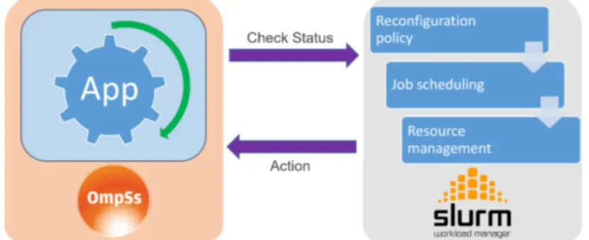
(6) mechanism. Thus, Slurm’s API allows us to resize a job following the next steps: • Job A has to be expanded 1. Submit a new job B with a dependency on the initial job A. Job B requests the number of nodes NB to be added to job A. 2. Update job B, setting its number of nodes to 0. This produces a set of NB allocated nodes which are not attached to any job. 3. Cancel job B. 4. Update job A and set its number of nodes to NA+NB. • Job A has to be shrunk 1. Update job A, setting the new number of nodes to the final size (NA is updated). After these steps, Slurm’s environment variables for job A are updated. These commands have no effect on the status of the running job, and the user still remains responsible for any malleability process and data redistribution.. Figure 1: Scheme of the interaction between the RMS and the runtime.. The framework we leverage consists of two main components: the RMS and the programming model runtime (see Figure 1). The RMS is aware of resource utilization and the queue of pending jobs. When an application is in execution, it periodically contacts the RMS, through the runtime, communicating its rescaling willingness (to expand or shrink the current number of allocated nodes). The RMS inspects the global status of the system to decide whether to initiate any rescaling action, and communicates this decision to the runtime. If the framework determines that a rescale action is beneficial 6.

(7) and possible, the RMS, runtime and application will collaborate to continue the execution of the application scaled to a different number of nodes (MPI processes). 4. Slurm Reconfiguration Policy We designed and developed a resource selection plug-in responsible for the reconfiguration decisions. This plug-in realizes a node selection policy featuring three modes that accommodate three degrees of scheduling freedom. 4.1. Request an Action Applications are allowed to “strongly suggest” a specific action. For instance, to expand the job, the user could set the “minimum” number of requested nodes to a value that is greater than the number of allocated nodes. However, Slurm will ultimately be responsible for granting the operation according to the overall system status. 4.2. Preferred Number of Nodes One of the parameters that applications can convey to the RMS is their preferred number of nodes to execute a specific computational stage. If the desired size corresponds to the current size, the RMS will return “no action”. If a “preference” is requested, and there is no outstanding job in the queue, the expansion can be granted up to a specified “maximum”. Otherwise, if the desired value is different from the current allocation, the RMS will try to expand or shrink the job to the preferred number of nodes. 4.3. Wide Optimization The cases not covered by the preceding methods are handled as follows: • A job is expanded if there are sufficient available resources to fulfill the new requirement of nodes and either (1) there is no job pending for execution in the queue, or (2) no pending job can be executed due to insufficient available resources. By expanding the job, we can expect it to finish its execution earlier and release the associated resources. • A job is shrunk if there is any queued job that could be executed by taking this action. More jobs in execution should increase the global throughput. Moreover, if the job is going to be shrunk, the queued job that has triggered the shrinking event will be assigned the maximum priority to foster its execution. 7.

(8) 5. Framework Design We implemented the necessary logic in Nanos++ to reconfigure jobs in tight cooperation with the RMS. In this section we discuss the extended API and the resizing mechanisms. 5.1. The Dynamic Management of Resources (DMR) API We designed the DMR API with two main functions: dmr check status and its asynchronous version dmr icheck status. These routines instruct the runtime (Nanos++) to communicate with the RMS (Slurm) in order to determine the resizing action to perform: “expand”, “shrink” or “no action”. The asynchronous counterpart schedules the next action for the following execution step, at the same time that the current step is executed. Hence, by skipping the action scheduling stage, the communication overhead in that step is avoided. In case an action is to be performed, these functions spawn a new set of processes and return an opaque handler. This API is exposed by the runtime and it is intended to be used by applications. Both functions need information about the scalability of the job, which has to provide the following input arguments: • Min: Minimum number of processes to be resized to. • Max : Maximum number of processes. This sets the maximum number of processes that the job can be scaled to. Minimum and maximum values define the limits of malleability. • Factor : Resizing factor (e.g., a factor of 2 will expand/shrink the number of processes to a value multiple/divisor of 2). • Pref : Preferred number of processes. The output arguments return the new number of nodes and a handler to be used in subsequent operations. An additional mechanism implemented to attain a fair balance between performance and throughput is the “scheduling inhibitor”. This introduces a timeout during which the calls to the DMR API are ignored. This knob is intended to be leveraged in iterative applications with short iteration intervals. The inhibition period can be tuned by means of an environment variable.. 8.

(9) 5.2. Automatic Job Reconfiguration The runtime will perform the following actions which leverage the Slurm resizing mechanisms (see Section 4) by means of its external API. 5.2.1. Expand A new resizer job (RJ) is first submitted requesting the difference between the current and total amount of desired nodes. This enables the original nodes to be reused. There is a dependency relation between the RJ and the original job (OJ). In order to facilitate complying with the RMS decisions, RJ is set to the maximum priority, facilitating its execution. The runtime waits until RJ moves from the “pending” to the “running” status. If the waiting time reaches a threshold, RJ is canceled and the action is aborted. This situation may occur if the RMS assigns the available resources to a different job during the scheduling action. This is more likely to occur in the asynchronous mode because an action can then experience some delay during which the status of the queue may change. Once OJ is reallocated, the updated list of nodes is gathered and used in a call to MPI Comm spawn to create a new set of processes. 5.2.2. Shrink The shrinking mechanism is slightly more complex than its expansion counterpart because Slurm kills all processes running in the released nodes. To prevent premature process termination, we need a synchronized workflow to guide job shrinking. Hence, the RMS sets a management node in charge of receiving an acknowledgment (ACK)from all other processes. These ACKs will signal that those processes completed their tasks and the node is ready to be released. After a scheduling is complete, the DMR call returns the expand–shrink action to be performed and the resulting number of nodes. The application is responsible for performing the appropriate actions using our programming model as described in Section 6. The spawning and termination of processes is managed by Nanos++ through the #pragma directive, which hides and triggers all the internal mechanisms for resource reallocation, process resize, data redistribution and resume of the execution.. 9.

(10) 1 2 3 4 5 6 7 8 9 10 11 12 13 14 15 16 17 18 19 20 21 22 23 24 25 26. v o i d main ( i n t argc , c h a r ∗∗ argv ) { ... int t = 0; M P I _ C o m m _ g e t _ p a r e n t (& parentComm ) ; i f ( parentComm == MPI_COMM_NULL ) { init ( data ) ; } else { MPI_Recv ( parentComm , data , myRank ) ; MPI_Recv ( parentComm , &t , myRank ) ; } compute ( data , t ) ; ... } v o i d compute ( data , t0 ) { f o r ( t=t0 ; t<timesteps ; t++) { nodeList = g e t _ n e w _ n o d e l i s t _ s o m e h o w ( ) ; i f ( nodelist != NULL ) { MPI_ Comm_spa wn ( myapp . bin , nodeList , &newComm ) ; MPI_Send ( newComm , data , myRank ) ; MPI_Send ( newComm , t , myRank ) ; exit ( 0 ) ; } compute_iter ( data , t ) ; } }. Listing 1: Pseudo-code of how a generic malleable application may look like using bare MPI.. 6. Programming Model In this section we review our programming model approach to address dynamic reconfiguration coordinated by the RMS. The programmability of our solution benefits from the OmpSs offload semantics, which presents an OpenMP-like syntax. 6.1. Benefits of the OmpSs Offload Semantics To showcase the benefits of the OmpSs offload semantics, we review the specific simple case of migration. This analysis allows us to focus on the fundamental differences between programming models because it does not involve data redistribution among a different number of nodes (which is of similar complexity in both models). MPI Migration. Listing 1 contains an excerpt of pseudo-code directly using MPI calls. In this case, we assume that some mechanism is available to determine the set of resources in line 17. 10.

(11) 1 2 3 4 5 6 7 8 9 10 11 12 13 14 15 16 17 18. v o i d main ( v o i d ) { ... int t = 0; init ( data ) ; compute ( data , t ) ; ... } v o i d compute ( data , t0 ) { f o r ( t=t0 ; t<timesteps ; t++) { action = d m r _ c h e c k _ s t a t us ( . . . , &newNnodes , &handler ) ; i f ( action ) { #pragma omp task inout ( data ) onto ( handler , myRank ) compute ( data , t ) } else compute_iter ( data ) ; } }. Listing 2: Pseudo-code of a generic malleable application using OmpSs and the DMR API.. OmpSs-based Migration. The same functionality is attained in Listing 2 by leveraging our proposal on top of the OmpSs offload semantics. This includes a call to our extended API in line 11. At a glance, our proposal exposes higher-level semantics, increasing code expressiveness and programming productivity. In addition, communication with the RMS is implicitly established in the call to the runtime in line 11, which pursues an increase in overall system resource utilization. Data transfers are managed by the runtime with the directive in line 13. Moreover, at this point, the initial processes terminates, letting the execution of “compute()” in line 14 continue in the processes of the new communicator identified by “handler”. 6.2. A Complete Example The excerpt of code in Listing 3 is derived from that showcased in Section 6.1 to discuss malleability. In this case the application must drive the task redistribution according to the resizing action. The mapping factor indicates the number of processes in the current set that are mapped to the processes in the new configuration (see Figure 2). This example implements homogeneous distributions, where we always resize to a multiple or a divisor of the current number of processes. Our model, however, supports arbitrary distributions. For the “expand” action (line 8), the original processes must partition the dataset. For instance, in Figure 2a, the processes split the dataset into 11.

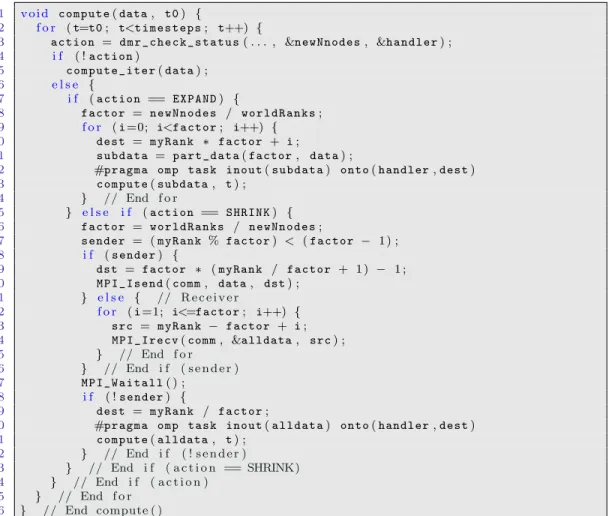
(12) 1 2 3 4 5 6 7 8 9 10 11 12 13 14 15 16 17 18 19 20 21 22 23 24 25 26 27 28 29 30 31 32 33 34 35 36. v o i d compute ( data , t0 ) { f o r ( t=t0 ; t<timesteps ; t++) { action = d m r _ c h e c k _ s t a t us ( . . . , &newNnodes , &handler ) ; i f ( ! action ) compute_iter ( data ) ; else { i f ( action == EXPAND ) { factor = newNnodes / worldRanks ; f o r ( i =0; i<factor ; i++) { dest = myRank ∗ factor + i ; subdata = part_data ( factor , data ) ; #pragma omp task inout ( subdata ) onto ( handler , dest ) compute ( subdata , t ) ; } // End f o r } e l s e i f ( action == SHRINK ) { factor = worldRanks / newNnodes ; sender = ( myRank % factor ) < ( factor − 1 ) ; i f ( sender ) { dst = factor ∗ ( myRank / factor + 1 ) − 1 ; MPI_Isend ( comm , data , dst ) ; } e l s e { // R e c e i v e r f o r ( i =1; i<=factor ; i++) { src = myRank − factor + i ; MPI_Irecv ( comm , &alldata , src ) ; } // End f o r } // End i f ( s e n d e r ) MPI_Waitall ( ) ; i f ( ! sender ) { dest = myRank / factor ; #pragma omp task inout ( alldata ) onto ( handler , dest ) compute ( alldata , t ) ; } // End i f ( ! s e n d e r ) } // End i f ( a c t i o n == SHRINK) } // End i f ( a c t i o n ) } // End f o r } // End compute ( ). Listing 3: Code example of how malleability is implemented in the computation function of a generic application using OmpSs and the DMR API.. #0 #1 Comm 1 #0 #1 Comm 2 (a) Expand from 2 to 4 processes.. (b) Shrink from 4 to 2 processes.. Figure 2: Example of the communication pattern among processes and communicators in the event of a reconfiguration.. 12.

(13) two subsets, mapping each half to a process in the new communicator. The data transfers are performed by the runtime according to the information included in the task offloading directive (line 12). The “shrink” action, on the other hand, involves preliminary explicit data movement. The processes in the original set are grouped into “senders” and “receivers”. This initial data movement within the initial communicator (Comm 1 ) is illustrated in the example in Figure 2b and is reflected in lines 17-27. Once the data is correctly placed in Comm 1, processes with the gathered data (“receivers”) utilize the #pragma directive to determine the inter-communicator communication pattern and the data dependencies to perform the data transfers (line 30). 7. Experimental Results In this section we evaluate the implementation of the malleability framework based on the DMR API via a set of workloads, fixed and malleable. 7.1. Workload Configuration The workloads were generated using the statistical model proposed by Feitelson [4], which characterizes rigid jobs based on observations from logs consisting of actual cluster workloads. For our purposes, we leverage the model customizing the following 2 parameters: • Jobs: Total number of jobs in the workload. • Arrival: Inter-arrival times of jobs modeled by a Poisson distribution of factor 10, which will prevent from receiving bursts of jobs while preserving a realistic job arrival pattern. 7.2. Platform Our evaluation was performed on the Marenostrum III supercomputer at Barcelona Supercomputing Center. Each compute node in this facility is equipped with two 8-core Intel Xeon E5-2670 processors running at 2.6 GHz and 128 GB of RAM. The nodes are connected via an InfiniBand Mellanox FDR10 network. For the software stack we used MPICH 3.2, OmpSs 15.06, and Slurm 15.08. Slurm was configured with the backfill job scheduling policy. Furthermore, we also enabled job priorities with the policy multifactor. Both were configured with default values. 13.

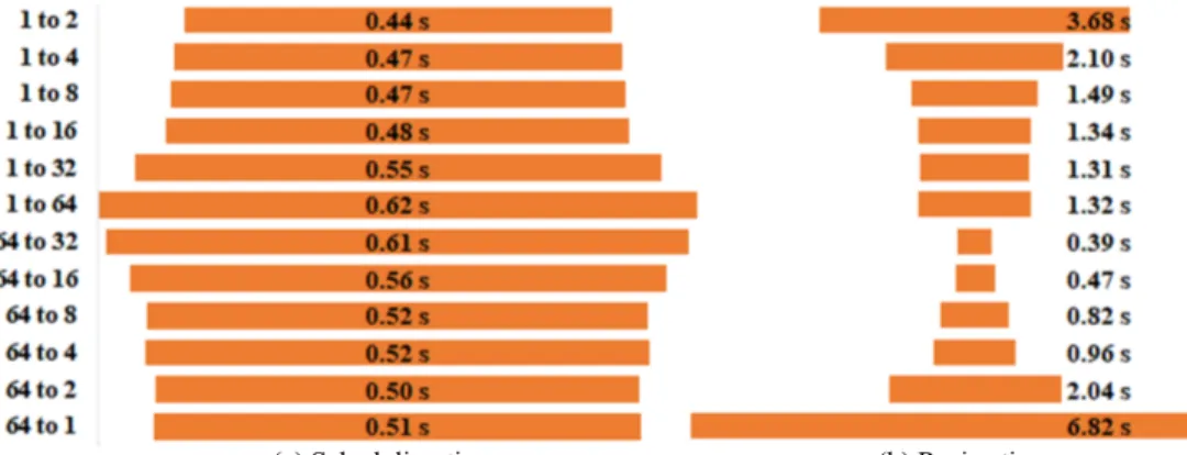
(14) 7.3. Reconfiguration Scheduling Performance Evaluation We next analyze the overhead of using our framework to enable malleability. For this purpose, we used the synthetic application Flexible Sleep (FS), configured to perform 2 steps and to transfer 1 GB of data during the reconfiguration. FS exhibits a perfectly linear scalability, hence, the minimum and maximum number of processes is set to 1 and 20 (the quantity of nodes used in this experiment), respectively. The main idea of this experiment is that each job executes an iteration, then it contacts with the RMS, and resumes the execution in the second step with the new configuration of processes. Figure 3 displays the temporal cost of several reconfigurations (y-axis) divided in stages (x-axis: (a) scheduling and (b)resize). The times in Figure 3 are obtained from the average of 10 executions for each reconfiguration. The left plot in that figure (a) shows the times taken by the RMS to determine an action (scheduling time). From top to bottom, the first half of the chart depicts the expansions, while the second half, the shrinks. The chart reveals a slight increment in the scheduling time when more nodes are involved in this process. The right plot of the same figure (b) shows the time that is necessary to perform the transfers among the processes. Two interesting behaviors are appreciated in this chart: • Increasing the number of processes involved in the reconfiguration, reduces the resize time. This is because the chunks of data are smaller and the time needed to concurrently transfer them is lower (compare the time of the reconfigurations 1 to 2 and 64 to 32 ). • Apart from the data redistribution, shrinks involve a more complex internal synchronization of processes. This complex synchronization is necessary to handle the way in which Slurm handles the processes when terminating. Hence, the time required to synchronize the processes augments with their numnber. In summary, Figure 3 seeks to highlight that the reconfiguration overhead increases when: more processes are involved (a); or the gap between the initial and final number of processes is greater (b). We have also studied the overhead in a more realistic workload, configuring FS to execute 25 steps instead of the 2 steps previously used for 14.

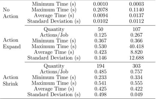
(15) ⠀ 愀 ⤀匀挀栀攀搀甀氀椀渀最琀椀洀攀 ⸀. ⠀ 戀⤀刀攀猀椀稀攀琀椀洀攀 ⸀. Figure 3: Analysis of the reconfiguration time per stages (scheduling (a) and resize (b)) for different number of processes.. analyzing the stages of a reconfiguration. Table 1 reports the statistics collected after executing a 400-job workload composed exclusively of those FS instances. The table is divided in three parts, and shows the actions taken and their run time during the workload execution in both synchronous and asynchronous scheduling. When no action is performed, the scheduling time is negligible (see average time and standard deviation of “no action”). The time increases when the RMS performs an action because of the scheduling process itself and the reconfiguration operations performed by the runtime. The first two rows of actions “expand” and “shrink” provide information about the number of reconfigurations scheduled per workload and per job. These results show that the synchronous version schedules fewer reconfigurations than the asynchronous. Since we are processing workloads with many queued jobs, running jobs are likely to be shrunk in favor of the pending jobs. For this reason “shrink” actions are more common. The table also demonstrates the negative effect of a timeout during an expansion. This effect is shown in the asynchronous scheduling column with the maximum, average and standard deviation values. In addition to the maximum time taken by the runtime to assert the expanding operation, these timeouts reveal a non-negligible dispersion in the duration values for the “expand” action. In fact, having such a high standard deviation turns the average time little representative.. 15.

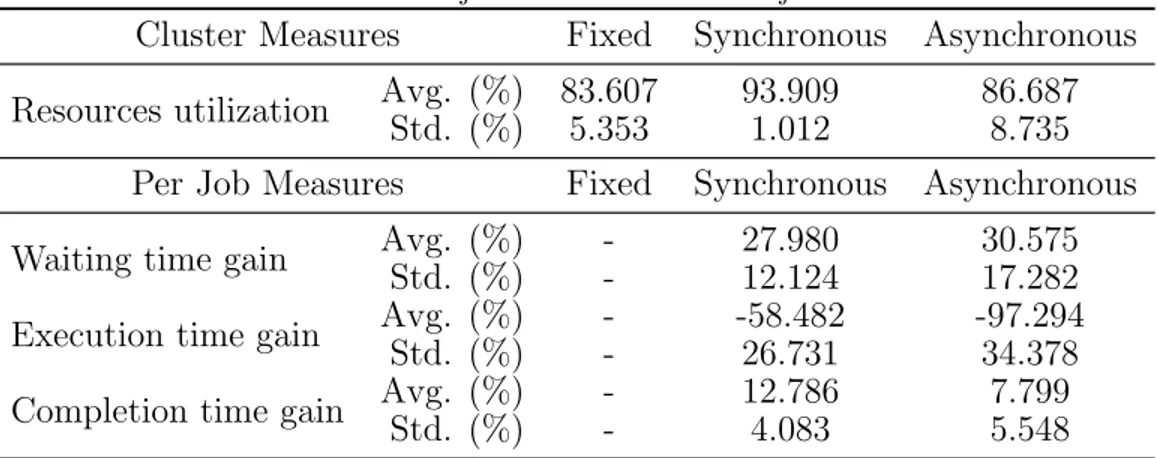
(16) Table 1: Analysis of the actions performed by the framework in a 400-job workload.. No Action. Minimum Time (s) Maximum Time (s) Average Time (s) Standard Deviation (s). Synchronous 0.0010 0.2078 0.0094 0.0102. Asynchronous 0.0003 0.1140 0.0137 0.0112. Action Expand. Quantity Actions/Job Minimum Time (s) Maximum Time (s) Average Time (s) Standard Deviation (s). 50 0.125 0.367 0.530 0.423 0.146. 107 0.267 0.366 40.418 8.820 12.688. Action Shrink. Quantity Actions/Job Minimum Time (s) Maximum Time (s) Average Time (s) Standard Deviation (s). 194 0.485 0.233 0.541 0.425 0.498. 303 0.757 0.334 0.555 0.422 0.049. 7.4. Dismissing the Asynchronous Scheduling In our previous work the asynchronous scheduling was reported to deliver worse performance than its synchronous counterpart [1]. This section thoroughly evaluates and compares both methods showing the inefficiency of the asynchronous scheduling for processing adaptive workloads exclusively composed of FS instances. Table 2 compares both modes, synchronous and asynchronous, in more detail, analyzing their performance at cluster and job levels. The most remarkable aspect here is that the synchronous scheduling occupies almost all the resources (' 94%) during the workload execution (the low standard deviation reveals that the mean value is barely unchanged for all sizes). The asynchronous mode still presents a higher utilization rate than the non-malleable workload. However, the high standard deviation means that the utilization is not as regular as in the synchronous case. In fact, this result hides a low average utilization for small workloads compared with a higher one for large workloads, similar to the synchronous scenario [1]. The last three rows offer timing measures: the wait-time of a job before initiating, the execution time of the job, and the difference of time from the job submission to its finalization (completion). Malleability provides an important reduction of the wait-time in both modes for all the sizes. This 16.

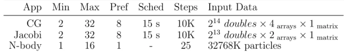
(17) Table 2: Cluster and job measures of the 400-job workloads.. Cluster Measures Resources utilization. Avg. (%) Std. (%). Per Job Measures Waiting time gain Execution time gain Completion time gain. Avg. Std. Avg. Std. Avg. Std.. Fixed. Synchronous. Asynchronous. 83.607 5.353. 93.909 1.012. 86.687 8.735. Fixed. Synchronous. Asynchronous. -. 27.980 12.124 -58.482 26.731 12.786 4.083. 30.575 17.282 -97.294 34.378 7.799 5.548. (%) (%) (%) (%) (%) (%). is because the resource manager can shrink a job in execution in favor of a queued one. With respect to the execution time, we experience a high degradation in the performance of individual jobs. For the synchronous scheduling, the negative gain of around a 58% is closely related to the fact that the application scales linearly. Thus, halving the resources produces a proportional reduction in performance. In the asynchronous scenario, the degradation is even more pronounced. The high standard deviation means that the performance of all the jobs is not equally impacted. Finally, the global job time (completion time) reveals malleability as an interesting feature, especially for the synchronous scheduling which completes the jobs, on average, 12% earlier than the traditional scenario. Since this test reveals no benefit from using the asynchronous scheduling, the rest of the experiments will exclusively use the synchronous mode. 7.5. Throughput Evaluation For our throughput evaluation we generated workloads of 50, 100, 200 and 400 jobs for both versions, fixed and malleable, all executed in 64 nodes of Marenostrum III. Each workload is composed of a set of randomly-sorted jobs (with a fixed seed), which instantiate one of the three non-synthetic applications: Conjugate Gradient (CG), Jacobi and N-body. The description of the applications and their behavior, as well as a thorough preliminary study of all the features implemented in the DMR API can be found in [1]. In summary, Table 3 gathers the reconfiguration parameters and the execution configuration of each application. Min, max and pref define the 17.

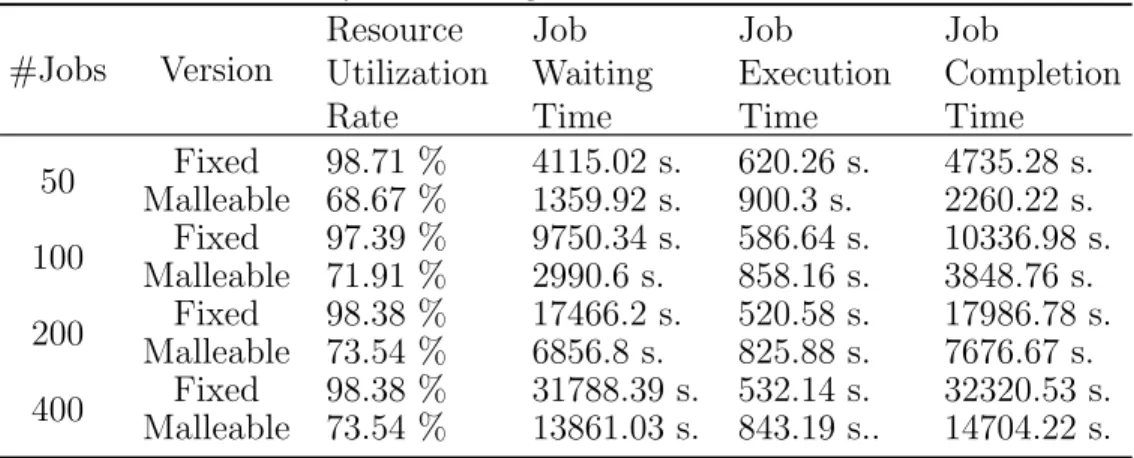
(18) Table 3: Configuration parameters for the applications. App Min Max Pref CG Jacobi N-body. 2 2 1. 32 32 16. 8 8 1. Sched Steps 15 s 15 s -. 10K 10K 25. Input Data 214 doubles × 4 arrays × 1 matrix 213 doubles × 2 arrays × 1 matrix 32768K particles. Number of jobs per workload. malleability parameters and sched is the scheduling period during which reconfigurations are inhibited (described in Section 5.1). Furthermore, the shrink-expand factor was set to 2 for all malleable jobs. It is worth noting that the input matrices are square. Following those parameters, each job is launched with its maximum number of processes, reflecting the user-preferred scenario of a fast execution. Figure 4 depicts the execution time of each workload comparing both configuration options: fixed and malleable. The labels at the end of the bars for the malleable workloads report the gain with respect to its fixed version. Table 4 details the measures extracted from the executions. In the first column, we compare the average resource utilization for fixed and malleable workloads. This rate corresponds to the average time when a node has been allocated by a job compared with the workload completion time. These results indicate that the malleable workloads reduce the allocation of nodes around 30%, offering more possibilities for jobs pending in the queue. 41.97%. 400. 41.42%. 200. Malleable. 49.04%. 100. Rigid 46.48%. 50 0. 10000. 20000 30000 40000 50000 Workload completion time (s). 60000. 70000. Figure 4: Workloads execution times (bars) and the gain of malleable workloads (bar labels).. 18.

(19) Table 4: Summary of the averaged measures from all the workloads.. #Jobs 50 100 200 400. Version Fixed Malleable Fixed Malleable Fixed Malleable Fixed Malleable. Resource Utilization Rate 98.71 % 68.67 % 97.39 % 71.91 % 98.38 % 73.54 % 98.38 % 73.54 %. Job Waiting Time 4115.02 s. 1359.92 s. 9750.34 s. 2990.6 s. 17466.2 s. 6856.8 s. 31788.39 s. 13861.03 s.. Job Execution Time 620.26 s. 900.3 s. 586.64 s. 858.16 s. 520.58 s. 825.88 s. 532.14 s. 843.19 s... Job Completion Time 4735.28 s. 2260.22 s. 10336.98 s. 3848.76 s. 17986.78 s. 7676.67 s. 32320.53 s. 14704.22 s.. Number of jobs per workload. The second column of Table 4 shows the average waiting time of the jobs for each workload. These times are illustrated in Figure 5, together with the gain rate for malleable workloads. The reduction around 60% reduction makes the job waiting time a crucial measure to consider from the perspective of throughput. In fact, this time is the main responsible for the reduction in the workload completion time. 56.40%. 400. 60.74%. 200. Malleable. 69.33%. 100. Rigid 66.95%. 50 0. 5000. 10000 15000 20000 25000 Avg. job waiting time (s). 30000. 35000. Figure 5: Average waiting time for all the jobs of each workload (bars) and the gain of malleable workloads (bar labels).. Table 4 also presents two more aggregated measures in the 400-job workload: The fifth column, with the average execution time; and the sixth, with the execution time plus the waiting time of the job, referred to as comple19.

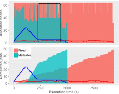
(20) tion time. The experiments show that jobs in the malleable workload are affected by the decrease in their number of processes. Nevertheless, this is compensated by the waiting time, which benefits their completion time. In order to understand the events during a workload execution, we have chosen the smallest workload to generate detailed charts and offer an in-depth analysis. The top and bottom plots in Figure 6 represent the evolution in time of the allocated resources and the number of completed jobs, respectively. The figure also shows the number of running jobs for fixed and malleable workloads (blue and red lines respectively). These demonstrate that the malleable workload utilizes fewer resources; furthermore, there are more jobs running concurrently (top chart). For both configurations, jobs are launched with the preferred number of processes (see Section 5.1); the fixed jobs obviously do not vary the amount of assigned resources, while in the malleable configuration, they are scaled-down as soon as possible. This explains the reduction of the utilization of resources. For instance, in the second half of the malleable shape in Figure 6 (marked area), we find a repetitive pattern in which there are 5 jobs in execution which allocate 40 nodes. The next eligible pending job in the queue needs 32 nodes to start. Therefore, unless one of the running jobs completes its execution, the pending job will not start, and the allocation rate will not grow. When a job eventually terminates its execution and releases 8 nodes, the scheduler initiates the job requesting 32 nodes. Now, there are 64 allocated nodes (the green peaks in the chart); however, as the job prefers 8 processes, it will be scaled-down. At the beginning of the trace in the bottom of Figure 6, the throughput of the fixed workload is higher than that of its counterpart: This occurs because the first jobs are completed earlier, since they have been launched with the best-performance number of processes. Meanwhile, in the malleable workload, many jobs are initiated (blue line) and, as soon as they terminate, the overall throughput experiences a notable improvement. Figure 7 depicts the execution and waiting time of each job grouped by application type. The execution time increases in the malleable workload for all cases. As mentioned earlier, jobs are shrunk to their preferred number of processes as soon as these are initiated. This implies a performance drop because of the reduction of resources. However, there is a job that leverages the benefits of an expansion. The last Jacobi job experiences an important drop of its execution time, since the completed jobs have deallocated their resources. 20.

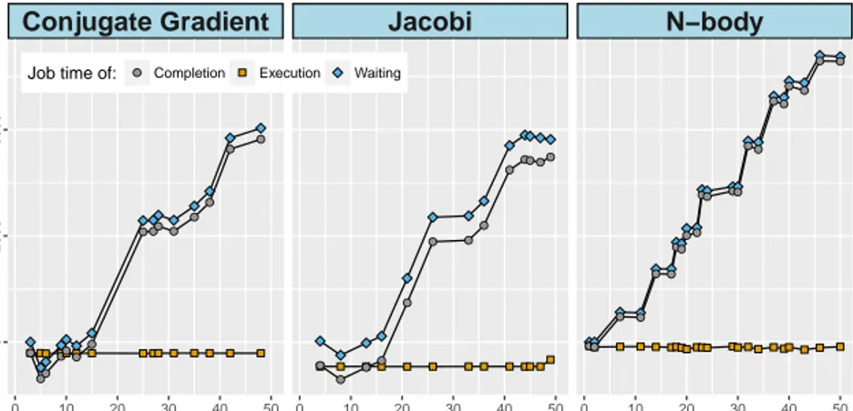
(21) Figure 6: Evolution in time for the 50-job workload. Blue and Red lines represent the running jobs for fixed and malleable workloads respectively.. At the beginning of the workload execution there is no remarkable difference in the waiting time of both versions: However, the emergence of new jobs continues and resources remain allocated for the running jobs in the fixed workload. The RMS cannot provide the means for processing faster the queue. For this reason, queued jobs in the fixed workload experience a considerable delay in initiating their execution. That difference of the fixed vs. malleable executions in the start time is crucial for the completion time of the job, as shown in Figure 8. This figure represents the difference in execution, waiting and completion time for each job grouped by application type. Again, the execution time remains below zero, which means that the difference is negative and the execution of the malleable workload is slower. Nevertheless, this small drawback is largely compensated by the waiting time. As reported, the completion difference time shows a heavy dependency on the waiting time, making it the main responsible for reducing the individual completion time, and in turn, the high throughput observed in the results.. 21.

(22) Jacobi. N−body ●. ● ● ● ● ● ●● ●●. ● ● ●. ● ● ● ● ●. ●. ●●. ●. ● ● ●●●● ●●●. ●● ● ● ● ●● ● ●. ●. ●. ●. ● ●. ●. ●. ● ●. ● ●● ● ●. Workload. ● ●● ●● ● ●. ● ●● ●. ● ●. ●. ● ●. ● ●● ●● ● ●. ● ●● ●. ● ●. ●. ● ●. ●. ●. ●. ● ●. ● ●● ● ●. ●● ●. 7500. ●. ●. 5000 2500. ● ●. ● ● ●. ●. ●. 0. ● ●. ●. ●● ● ●. ●. ●●. ● ● ● ●● ● ● ● ●. ●. ●●. ●● ●●. ●. ● ●. ● ● ●. 10. ●. ●●. ●. ●. 0. ● ● ● ●●. ●. ●. ●● ●●. ●. ●. ● ●●. ● ● ● ● ● ●●. Malleable. ●. ●. ●. Fixed. ●. ●. ●. ●●. ●. ●. ●. Waiting time (s.). ●●. 1000. ●. 500. Execution time (s.). Conjugate Gradient. 20. 30. 40. 50. 0. ●●. 10. 20. 30. 40. 50. ●. ●. ●. ●● ● ● ●●●● ●. 0. 10. 20. 30. 40. 50. Job Id.. Figure 7: Execution (top) and waiting (bottom) times of each job grouped by application type (columns).. Conjugate Gradient. Jacobi. N−body ●. ●. Completion. Execution. ●. Waiting. 5000. ● ● ●●. ●. ● ●. ●●. ●● ● ● ●●. ●. 2500. Difference time (s.). Job time of:. ● ●● ●. ●. ●. ●● ●●. ●. ●. ●●. ● ● ●. 0. ● ● ● ●. ●. ● ●. ●●. 0. ●. ●● ●. ●. ●. 10. 20. 30. 40. 50. 0. 10. 20. 30. 40. 50. 0. 10. 20. 30. 40. 50. Job Id.. Figure 8: Completion, execution and waiting time difference of the fixed vs. malleable executions for each job.. 22.

(23) 8. Conclusions This paper improves the state–of–the–art in dynamic job reconfiguration by targeting the global throughput of a high performance facility. We benefit from already-existing, first-class software components to design our novel approach that introduces a dynamic reconfiguration mechanism for malleable jobs, composed of two modules: the runtime and the resource manager. Those two elements collaborate to resize jobs on–the–fly to favor the global throughput of the system. As we prove in this paper, our approach can significantly improve resource utilization while, at the same time, reducing the waiting time for enqueued jobs, and decreasing the total execution time of workloads. Although this is achieved at the expense of a certain increase in the job execution time, we have reported that, depending on the scalability of the application, this drawback can be negligible. The malleability framework can be downloaded from: https://bitbucket.org/account/user/ompssmalleability/projects/FS. The malleable applications can be downloaded from: https://bitbucket.org/account/user/ompssmalleability/projects/MA. Acknowledgments The authors would like to thank the anonymous reviewers for their valuable and insightful comments that improved the quality of this paper. This work is supported by the projects TIN2014-53495-R and TIN2015-65316-P from MINECO and FEDER. This project has received funding from the European Union’s Horizon 2020 research and innovation programme under the Marie Sklodowska Curie grant agreement No. 749516 References [1] S. Iserte, R. Mayo, E. S. Quintana-Ortı́, V. Beltran, A. J. Peña, Efficient scalable computing through flexible applications and adaptive workloads, in: 10th International Workshop on Parallel Programming Models and Systems Software for High-End Computing (P2S2), Bristol, UK, 2017. [2] A. B. Yoo, M. A. Jette, M. Grondona, SLURM: Simple Linux utility for resource management, in: 9th International Workshop on Job Scheduling Strategies for Parallel Processing (JSSPP), 2003, pp. 44–60. 23.

(24) [3] F. Sainz, J. Bellon, V. Beltran, J. Labarta, Collective offload for heterogeneous clusters, in: 22nd International Conference on High Performance Computing (HiPC), 2015. [4] D. G. Feitelson, L. Rudolph, Toward convergence in job schedulers for parallel supercomputers, in: Job Scheduling Strategies for Parallel Processing, Vol. 1162/1996, 1996, pp. 1–26. [5] J. Padhye, L. Dowdy, Dynamic versus adaptive processor allocation policies for message passing parallel computers: An empirical comparison, in: Job Scheduling Strategies for Parallel Processing, 1996, pp. 224–243. [6] K. El Maghraoui, T. J. Desell, B. K. Szymanski, C. A. Varela, Malleable iterative MPI applications, Concurrency and Computation: Practice and Experience 21 (3) (2009) 393–413. [7] P. Lemarinier, K. Hasanov, S. Venugopal, K. Katrinis, Architecting malleable MPI applications for priority-driven adaptive scheduling, in: Proceedings of the 23rd European MPI Users’ Group Meeting, 2016. [8] A. Moody, G. Bronevetsky, K. Mohror, B. R. de Supinski, Design, modeling, and evaluation of a scalable multi-level checkpointing system, in: ACM/IEEE International Conference for High Performance Computing, Networking, Storage and Analysis (SC10), 2010. [9] W. Bland, A. Bouteiller, T. Herault, G. Bosilca, J. Dongarra, Postfailure recovery of MPI communication capability: Design and rationale, International Journal of High Performance Computing Applications 27 (3) (2013) 244–254. [10] A. Gupta, B. Acun, O. Sarood, L. V. Kalé, Towards realizing the potential of malleable jobs, in: 21st International Conference on High Performance Computing (HiPC), 2014. [11] F. S. Ribeiro, A. P. Nascimento, C. Boeres, V. E. F. Rebello, A. C. Sena, Autonomic malleability in iterative MPI applications, in: Symposium on Computer Architecture and High Performance Computing, 2013. [12] G. Martı́n, D. E. Singh, M. C. Marinescu, J. Carretero, Enhancing the performance of malleable MPI applications by using performance-aware dynamic reconfiguration, Parallel Computing 46. 24.

(25) [13] G. Martı́n, M. C. Marinescu, D. E. Singh, J. Carretero, FLEX-MPI: an MPI extension for supporting dynamic load balancing on heterogeneous non-dedicated systems, in: Euro-Par Parallel Processing, 2013. [14] R. Sudarsan, C. J. Ribbens, ReSHAPE: A framework for dynamic resizing and scheduling of homogeneous applications in a parallel environment, in: International Conference on Parallel Processing, 2007. [15] R. Sudarsan, C. Ribbens, Scheduling resizable parallel applications, in: International Symposium on Parallel & Distributed Processing, 2009. [16] R. Sudarsan, C. J. Ribbens, D. Farkas, Dynamic resizing of parallel scientific simulations: A case study using LAMMPS, in: International Conference on Computational Science (ICCS), 2009, pp. 175–184. [17] R. Sudarsan, C. J. Ribbens, Combining performance and priority for scheduling resizable parallel applications, Journal of Parallel and Distributed Computing 87 (2016) 55–66. [18] S. Prabhakaran, M. Neumann, S. Rinke, F. Wolf, A. Gupta, L. V. Kale, A batch system with efficient adaptive scheduling for malleable and evolving applications, in: IEEE International Parallel and Distributed Processing Symposium, 2015, pp. 429–438.. 25.

(26)