Development of a Vapor Compression Cicle heat Pump model using EES Example of application for heat recovery

Texto completo

(1)ESCUELA SUPERTIOR DE TECNOLOGÍA Y CIENCIAS EXPERIMENTALES. Departamento de Ingeniería Mecánica y Construcción. Development of a Vapor Compression Cycle Heat Pump model using EES. Example of application for heat recovery Héctor Torres Emo. Directors: Joaquín Navarro Esbrí Francisco Molés Ribera. Final Degree’s Work Grado en Ingeniería Mecánica Castellón de la Plana, septiembre de 2017.

(2) Project Documents Section 1 – Project Report Section 2 – Budget Section 3 – Schedule of conditions Section 4 – Annexes Section 5 – Blueprints. 1 75 79 85 99.

(3)

(4) Section 1 – Project Report. 1.

(5) Report index 1.. INTRODUCTION ................................................................................................................................ 9 1.1. 1.2. 1.3.. 2.. JUSTIFICATION ...............................................................................................................................11 OBJECTIVE ....................................................................................................................................11 METHODOLOGY .............................................................................................................................11. BACKGROUND ................................................................................................................................ 12 2.1. HEAT PUMP ..................................................................................................................................12 2.2. HEAT RECOVERY APPLICATIONS ........................................................................................................13 2.3. THERMODYNAMIC CYCLE .................................................................................................................17 2.4. MAIN COMPONENTS ......................................................................................................................21 2.4.1. Compressor .......................................................................................................................21 2.4.2. Expansion device ..............................................................................................................24 2.4.3. Heat exchanger ................................................................................................................24 2.4.4. Safety and control devices ................................................................................................26 2.5. WORKING FLUIDS ...........................................................................................................................26. 3.. MODEL ........................................................................................................................................... 32 3.1. SYSTEM DESCRIPTION .....................................................................................................................32 3.2. STARTING HYPOTHESES....................................................................................................................33 3.3. COMPONENTS MODELLING...............................................................................................................33 3.3.1. Compressor .......................................................................................................................34 3.3.2. Expansion Device ..............................................................................................................34 3.3.3. Heat Exchangers ...............................................................................................................34 3.4. PERFORMANCE INDICATORS .............................................................................................................42. 4.. RESULTS AND ANALYSIS ................................................................................................................. 43 4.1. SIMULATION PARAMETERS ...............................................................................................................43 4.2. RESULTS REPRESENTATION AND ANALYSIS ...........................................................................................45 4.2.1. Cycle Parameters ..............................................................................................................45 4.2.2. Components Parameters ..................................................................................................57. 5.. CONCLUSIONS ................................................................................................................................ 69 5.1. 5.2. 5.3.. 6.. PROJECT CONCLUSIONS ...................................................................................................................69 FURTHER DEVELOPMENTS ................................................................................................................71 PERSONAL CONCLUSIONS .................................................................................................................71. BIBLIOGRAPHY ............................................................................................................................... 72. 2.

(6) FIGURE INDEX FIGURE 1 GLOBAL GREENHOUSE GAS EMISSIONS SINCE 1990 ...................................................................................... 9 FIGURE 2 DERIVED HEAT PRODUCTION IN THE EU SINCE 1990. DATA SOURCE: EUROSTAT ............................................... 10 FIGURE 3 HEAT PUMP SCHEME ............................................................................................................................. 12 FIGURE 4 HEAT DEMAND QUALITY AND QUANTITY IN EUROPEAN MARKETS BY INDUSTRY. SOURCE: NELLISSEN AND WOLF, 2015 .............................................................................................................................................................. 14 FIGURE 5 ZNEH SCHEMATIC REPRESENTATION. ........................................................................................................ 15 FIGURE 6 SIMPLE CONFIGURATION......................................................................................................................... 18 FIGURE 7 INTERNAL HEAT EXCHANGER CONFIGURATION ............................................................................................ 19 FIGURE 8 TWO-STAGE COMPRESSOR CONFIGURATION ............................................................................................... 20 FIGURE 9 CASCADE CONFIGURATION ...................................................................................................................... 21 FIGURE 10 RECIPROCATING COMPRESSOR............................................................................................................... 22 FIGURE 11 SCROLL COMPRESSOR .......................................................................................................................... 22 FIGURE 12 SCREW COMPRESSOR .......................................................................................................................... 22 FIGURE 13 COMPRESSOR TYPES AND RANGE OF OPERATION........................................................................................ 23 FIGURE 14 EXPANSION VALVE .............................................................................................................................. 24 FIGURE 15 HEAT EXCHANGERS: SHELL AND TUBE (LEFT) AND PLATE EXCHANGERS (RIGHT). ............................................... 25 FIGURE 16 DIAGRAM OF A CONCENTRIC CYLINDRICAL EXCHANGER .............................................................................. 25 FIGURE 17 SAFETY DEVICES.................................................................................................................................. 26 FIGURE 18 TIMELINE OF REFRIGERANTS DEVELOPMENT .............................................................................................. 28 FIGURE 19 MODEL EVOLUTION ............................................................................................................................. 32 FIGURE 20 MODEL SCHEME ................................................................................................................................. 32 FIGURE 21 CONCENTRIC HEAT EXCHANGER GEOMETRY ............................................................................................. 35 FIGURE 22 HEAT EXCHANGER TEMPERATURE SCHEME ............................................................................................... 36 FIGURE 23 EVAPORATOR STAGES........................................................................................................................... 39 FIGURE 24 CONDENSER STAGES ............................................................................................................................ 40. TABLE INDEX TABLE 1 COMMERCIAL HEAT PUMP SYSTEMS............................................................................................................ 14 TABLE 2 HEAT PUMP INDUSTRIAL APPLICATIONS ....................................................................................................... 16 TABLE 3 SAFETY GROUP CLASIFFICATION ................................................................................................................. 28 TABLE 4 FLUIDS PROPERTIES AND INFORMATION....................................................................................................... 29 TABLE 5 R134A/R1234YF/R1234ZEE DATA. VALUES FOR CRITICAL PRESSURE AND CRITICAL TEMPERATURE FROM COOLPROP FLUIDS PROPERTIES, PURE AND PSEUDO-PURE FLUID PROPERTIES. ...................................................................... 30 TABLE 6 SYSTEM MODELLING PARAMETERS ............................................................................................................. 33 TABLE 7 COMPRESSOR MODELLING PARAMETERS...................................................................................................... 34 TABLE 8 EVAPORATOR MODELLING PARAMETERS ...................................................................................................... 39 TABLE 9 CONDENSER MODELLING PARAMETERS........................................................................................................ 40 TABLE 10 SIMULATION PARAMETERS ..................................................................................................................... 43. 3.

(7) DIAGRAM INDEX DIAGRAM 1 REVERSE CARNOT CYCLE EXAMPLE FOR R134A........................................................................................ 17 DIAGRAM 2 IHX CYCLE ........................................................................................................................................ 20 DIAGRAM 3 PT CHART FOR SEVERAL REFRIGERANTS AT SATURATION. DATA SOURCE: COOLPROP ....................................... 29 DIAGRAM 4 R12/R134A/R1234ZE(E)/R1234YF DATA SOURCE: COOLPROP .............................................................. 31 DIAGRAM 5 PRESSURE-ENTHALPY GRAPH FOR R134A/R1234YF/R1234ZEE DATA SOURCE: COOLPROP ........................... 31 DIAGRAM 6 T-S GRAPH OF THE CYCLE WITH SECONDARY FLUIDS. SOURCE: EES............................................................... 44 DIAGRAM 7 P-H GRAPH OF THE CYCLE. SOURCE: EES ................................................................................................ 44 DIAGRAM 8 COP SIMULATION 1 ........................................................................................................................... 45 DIAGRAM 9 CONDENSER POWER SIMULATION 1....................................................................................................... 46 DIAGRAM 10 COMPRESSOR POWER SIMULATION 1 .................................................................................................. 46 DIAGRAM 11 COP SIMULATION 2 ......................................................................................................................... 47 DIAGRAM 12 CONDENSER POWER SIMULATION 2 .................................................................................................... 47 DIAGRAM 13 COMPRESSOR POWER SIMULATION 2 .................................................................................................. 48 DIAGRAM 14 COP SIMULATION 3 ......................................................................................................................... 48 DIAGRAM 15 CONDENSER POWER SIMULATION 3 .................................................................................................... 49 DIAGRAM 16 COMPRESSOR POWER SIMULATION 3 .................................................................................................. 49 DIAGRAM 17 CR SIMULATION 1 ............................................................................................................................ 50 DIAGRAM 18 VOLUMETRIC FLOW SIMULATION 1 ...................................................................................................... 51 DIAGRAM 19 MASS FLOW SIMULATION 1 ............................................................................................................... 51 DIAGRAM 20 DISCHARGE TEMPERATURE SIMULATION 1 ............................................................................................ 52 DIAGRAM 21 CR SIMULATION 2 ............................................................................................................................ 52 DIAGRAM 22 VOLUMETRIC FLOW SIMULATION 2 ...................................................................................................... 53 DIAGRAM 23 MASS FLOW SIMULATION 2 ............................................................................................................... 53 DIAGRAM 24 DISCHARGE TEMPERATURE SIMULATION 2 ............................................................................................ 54 DIAGRAM 25 CR SIMULATION 3 ............................................................................................................................ 54 DIAGRAM 26 VOLUMETRIC FLOW SIMULATION 3 ...................................................................................................... 55 DIAGRAM 27 MASS FLOW SIMULATION 3 ............................................................................................................... 55 DIAGRAM 28 DISCHARGE TEMPERATURE SIMULATION 3 ............................................................................................ 56 DIAGRAM 29 CONDENSER EXCHANGE AREA SIMULATION 1 ......................................................................................... 57 DIAGRAM 30 EVAPORATOR EXCHANGE AREA SIMULATION 1 ....................................................................................... 58 DIAGRAM 31 IHX EXCHANGE AREA SIMULATION 1 .................................................................................................... 58 DIAGRAM 32 CONDENSER EXCHANGE AREA SIMULATION 2 ......................................................................................... 59 DIAGRAM 33 EVAPORATOR EXCHANGE AREA SIMULATION 2 ....................................................................................... 59 DIAGRAM 34 IHX EXCHANGE AREA SIMULATION 2 .................................................................................................... 60 DIAGRAM 35 CONDENSER EXCHANGE AREA SIMULATION 3 ......................................................................................... 60 DIAGRAM 36 EVAPORATOR EXCHANGE AREA SIMULATION 3 ....................................................................................... 61 DIAGRAM 37 IHX EXCHANGE AREA SIMULATION 3 .................................................................................................... 61 DIAGRAM 38 CONDENSER PRESSURE DROP SIMULATION 1 ......................................................................................... 62 DIAGRAM 39 EVAPORATOR PRESSURE DROP SIMULATION 1 ........................................................................................ 62 DIAGRAM 40 IHX EXTERNAL TUBE PRESSURE DROP SIMULATION 1 ............................................................................... 63 DIAGRAM 41 IHX INTERNAL PRESSURE DROP SIMULATION 1 ....................................................................................... 63 DIAGRAM 42 CONDENSER PRESSURE DROP SIMULATION 2 ......................................................................................... 64 DIAGRAM 43 EVAPORATOR PRESSURE DROP SIMULATION 2 ........................................................................................ 64 DIAGRAM 44 IHX EXTERNAL TUBE PRESSURE DROP SIMULATION 2 ............................................................................... 65 DIAGRAM 45 IHX INTERNAL TUBE PRESSURE DROP SIMULATION 2 ............................................................................... 65 DIAGRAM 46 CONDENSER PRESSURE DROP SIMULATION 3 ......................................................................................... 66 DIAGRAM 47 EVAPORATOR PRESSURE DROP SIMULATION 3 ........................................................................................ 66 DIAGRAM 48 IHX EXTERNAL TUBE PRESSURE DROP SIMULATION 3 ............................................................................... 67 DIAGRAM 49 IHX INTERNAL TUBE PRESSURE DROP SIMULATION 3 ............................................................................... 67. 4.

(8) EQUATION INDEX EQUATION 1 CARNOT COP WITH TEMPERATURES..................................................................................................... 17 EQUATION 2 HEAT PUMP COP ............................................................................................................................. 17 EQUATION 3 THERMAL POWER ............................................................................................................................. 18 EQUATION 4 MODEL COP ................................................................................................................................... 34 EQUATION 5 COMPRESSOR POWER ....................................................................................................................... 34 EQUATION 6 VOLUMETRIC CAPACITY OF THE COMPRESSOR ........................................................................................ 34 EQUATION 7 ISENTROPIC PERFORMANCE INTERACTION .............................................................................................. 34 EQUATION 8 HEAT TRANSFER BETWEEN FLUIDS ........................................................................................................ 35 EQUATION 9 LOGARITHMIC MEAN TEMPERATURE AVERAGE ...................................................................................... 35 EQUATION 10 TEMPERATURE DIFFERENCE A ........................................................................................................... 35 EQUATION 11 TEMPERATURE DIFFERENCE B ........................................................................................................... 35 EQUATION 12 GLOBAL HEAT TRANSFER COEFFICIENT................................................................................................ 36 EQUATION 13 CONVECTION THERMAL RESISTANCE .................................................................................................. 36 EQUATION 14 CONDUCTION THERMAL RESISTANCE .................................................................................................. 36 EQUATION 15 GLOBAL THERMAL RESISTANCE ......................................................................................................... 36 EQUATION 16 RELATIONSHIP BETWEEN LENGTH AND HEAT TRANSFER ........................................................................... 36 EQUATION 17 REYNOLDS NUMBER ........................................................................................................................ 37 EQUATION 18 PRANDTL NUMBER ......................................................................................................................... 37 EQUATION 19 HEAT TRANSFER COEFFICIENT FOR SINGLE PHASE .................................................................................. 37 EQUATION 20 GNIELINSKI CORRELATION FOR NUSSELT NUMBER.................................................................................. 37 EQUATION 21 FRICTION FACTOR ........................................................................................................................... 37 EQUATION 22 DARCY-WEISBACH CORRELATION ....................................................................................................... 38 EQUATION 23 IHX POWER ................................................................................................................................... 38 EQUATION 24 IHX EFFICIENCY PARAMETER ............................................................................................................. 38 EQUATION 25 EVAPORATOR POWER ...................................................................................................................... 39 EQUATION 26 CONDENSER POWER ....................................................................................................................... 40 EQUATION 27 DITTUS-BOELTER CORRELATION ........................................................................................................ 40 EQUATION 28 GUNGOR-WINTERTON CORRELATION ................................................................................................. 41 EQUATION 29 QUALITY INCREASE FACTOR............................................................................................................... 41 EQUATION 30 QUALITY INCREASE FACTOR MODIFIER ................................................................................................. 41 EQUATION 31 SUPPRESSION FACTOR...................................................................................................................... 41 EQUATION 32 SUPPRESSION FACTOR MODIFIER ........................................................................................................ 41 EQUATION 33 FROUDE NUMBER ........................................................................................................................... 41 EQUATION 34 BOILING NUMBER........................................................................................................................... 41 EQUATION 35 SHAH CORRELATION ........................................................................................................................ 41 EQUATION 36 SHAH QUALITY FACTOR .................................................................................................................... 42 EQUATION 37 PIERRE CORRELATION ...................................................................................................................... 42 EQUATION 38 FRICTION FACTOR FOR PHASE CHANGE ................................................................................................ 42 EQUATION 39 FRICTION FACTOR QUALITY MODIFIER ................................................................................................. 42 EQUATION 40 COMPRESSOR RATIO........................................................................................................................ 43. 5.

(9) NOMENCLATURE Symbol – Letter. Parameter and unit. P. Pressure [Pa]. W. Compressor power [W]. s. Entropy [J/Kg·K]. T. Temperature [K]. q. Quality [-]. 𝑚𝑚̇. Mass flow rate [Kg/s]. Nu. Nusselt number [-]. 𝑄𝑄̇. Thermal power [W]. h. Enthalpy [J/Kg]. Bo. Boiling number [-]. Re. Reynolds number [-]. Frlo. Froude number [-]. Pr. Prandtl number [-]. D. Diameter [m]. cp. Specific heat [J/Kg·K]. v. Velocity [m/s]. α. Heat transfer coefficient [W/m2·K]. υ. Specific volume [m3/Kg]. S. Suppression factor [-]. U. Global heat transfer coefficient [W/m2·K]. G. Mass velocity [Kg/s·m2]. L. Length [m]. f. Friction factor [-]. Δ. Increment applied to a parameter [-]. ρ. Density [Kg/m3]. ε. Efficiency parameter [-]. k. Thermal conductivity [W/m·K]. Z. Shah coefficient [-]. g. Gravity [m/s2]. A. Area [m2]. V. Volume [m3]. η. Performance indicator [-]. µ. Dynamic viscosity [Pa·s]. F. Increase factor [-]. R. Thermal resistance [-]. CR. Compression Ratio [-] 6.

(10) SUB-INDEX NOMENCLATURE Sub index. Parameter and unit Hydraulic diameter. hyd. Exterior. ext. Outer. out. in, int. Interior. c, cond. Condenser. Inner. inn e, evap. Evaporator. IHX. Internal heat exchanger. is vol. Isentropic. fg. Fluid to gas. Secondary fluid. sf. glob. Global. crit. Critical. Volumetric Mid-point. m. 7.

(11) 8.

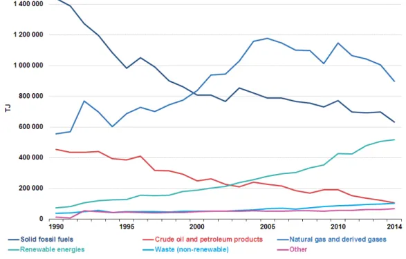
(12) 1. Introduction Since the mid-20th century around the world the generation of energy has increased, associate to the electricity generation with coal and hydrocarbon products. Due to this extensive generation, the planet is now suffering what it has been called the climate change, in which two factors are fundamental: the decreasing in area and thickness of the ozone layer and the increase of temperature in the hole planet due to the greenhouse effect, powered by the emissions of greenhouse gases to the atmosphere. In Figure 1 a graphical representation of the percentages of emissions due to energy production is shown.. Figure 1 Global Greenhouse Gas Emissions since 1990. Those two factors triggered the response of the society and governments started legislating to reduce the production and emission of the substances responsible. The answer to this were the several different treaties signed about the emission of substances with high Global Warming Potential (GWP) and high Ozone Depletion Potential (ODP). This substances have been regulated with the Montreal Protocol [1] and with the Kyoto Protocol [2], which has been updated with the Paris Agreement [3]. In the EU what regulates the fluids from the GWP point of view is the F-Gas Regulation [4]. Also introduced by those articles is the concept of Energy Efficiency; which applies to an industry, a building or a machine, and highlights the usage of the energy made by the system in which is applied. It determines if a system, e.g. an industry, is using the energy that consumes with a profit or if is usage is over the parameters and wasted. The governments and institutions use this as an indicator to allocate penalties and bills to the industry with low energy efficiency parameters. In the EU, the production of heat (see Figure 2) can be traced from the fuel used, and the effects of 9.

(13) this policies about energy efficiency and greenhouse gases regulation is a decrease in the usage of traditional methods for heat generation and an increase in the use of new technologies like renewable energies.. Figure 2 Derived heat production in the EU since 1990. Data Source: Eurostat. Nowadays the high demand in heat energy is provided by fossil fuels and derived products, generating at the same time a huge amount of waste heat. This waste affects directly to the environment, both with the residual gases from the generation (NOx, SOx, CO2) and with the heat itself, affecting the surrounding ecosystem of the industry. The possibility of recovery this wasted heat represents a measure of energy saving and efficiency as well as contributing with notable benefits in energy, environmental and economic terms. Reducing the impact on the climate change and the need for better energy management by the industries and systems, e.g. hospitals, administration buildings, offices; create a need for the systems which recycle energy from sources before considered waste. Those systems, where the Heat Pump (HP) emerges as a viable solution, are the main object of study by R&D groups and companies in the energy saving field. This field focus is the development of systems to decrease the usage of common heat production systems (e.g. boilers, which consumes a high amount of fuel and are expensive to operate and maintain) and recycle the heat generated or wasted, increasing the overall efficiency and helping to reduce the ecological footprint of the overall system. Systems like the HP can take profit of the heat wasted by the processes of heat generation, considered as a major problem for the companies, using this heat for a useful application. The heat waste can be directly redirected when the temperature is high enough, if this temperature isn’t high enough a heat pump is presented as a solution. The heat pump is capable of recover a low temperature heat and take it to the desired conditions of consumption. A major part of the heat pump technology developed is based on the Vapor Compression Cycle Heat Pump (VCCHP), either working at temperatures up to 90ºC. The VCCHP allows to transfer heat from different sources with an input of mechanical energy via compression. 10.

(14) In the recent years of investigation, the VCCHP are bounded to the generation of electricity with renewables sources, e.g. solar panels and batteries, to provide a full system for energy recovery with the minimum impact on the environment. [5] The development in the energy saving field focused not only on the systems and the components, but also in the working fluids used, which in last terms, are the key of this systems allowing them to operate at different temperatures and limit the geometry and characteristics of the components. The fields of operation for this technology it’s wide and comprehend a great variety of different fields, each one of it with their needs and specifications. Thus, an extensive range of components and fluids has been created and which need to be tested and analysed before installed, because the heat recovery systems are not a cheap and require an exhaustive study for each application. In order to develop efficient systems, new methods had to be developed due to the quantity of possible iterations for a single application, the increase in the number of working fluids and the range of components available. Data bases has been created with the characteristics of the fluids, which helps to calculate and examine those fluids allowing to model and compare different cycles, systems and components.. 1.1.Justification. Due to the possibility of use residual energy through a heat pump, it is analysed this technology to apply it in the energy recovery, from waste or natural sources, to enhance efficiency in the heat production. This technology developed focused on the Heat Pump systems, which allow to make the most of the low temperature residual heat in heat demanding processes and thus reducing the need of traditional heat generation systems. In this Final Degree’s Work, the Heat Pump system will be treated as a valid method to recover energy from residual heat sources before considered waste. In these terms, the study will also focus on the usage of new low-GWP fluids as substitute for the previous refrigerants.. 1.2.Objective. The general objective is the study, using models of Vapor Compression Cycle Heat Pump (VCCHP) systems for the recovery of residual heat recovery and the evaluation of Low-GWP working fluids as an alternative. The specific objectives of the work are: • • • •. Background review. Heat Pump model for testing. Analysis of performance parameters from different fluids. Analysis of components.. 1.3. Methodology. To achieve the objectives previously set a methodology based on the development of the HP model is proposed. The model will be used to test the different alternative fluids and, therefore, the evaluation and analysis of the results.. 11.

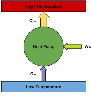
(15) Thus, the present document is organised: • • • • •. Present chapter: Introduction. Stablishing the key factors for the HP technology and the social and economic base where stands. Chapter 2: Background. Reviewing the technology conforming the HP system and the components of it as well as the fluids used to operate and the evolution of them. Chapter 3: Model. Defining the hypotheses and mathematical methods used in the HP modelling and the starting data and format of the results. Chapter 4: Results. Gathering the results given by the model in the simulations and comparing the key performance parameters for the iterations done. Chapter 5: Conclusions. Reviewing the results and stablishing connections with the background and applications for the technology studied.. Therefore, the work developed here contributes to help this field of development with an iterative mathematical model for VCCHP systems using Engineering Equation Solver (EES) software [6] and the CoolProp libraries [7] which can simulate under different work conditions several different refrigerants in order to gather data from them and allowing the analysis and comparison.. 2. Background 2.1.Heat Pump. The Heat Pump system analysed is based on the vapor compression cycle, using a compressor, a condenser, an expansion valve and an evaporator in the simplest configuration. The heat pump allows to transfer heat between external fluids, one of them as the source and the other as the sink, using electric energy via compression of the working fluid, as shown on Figure 3. The efficiency of a heat pump is measured as the heat provided by it in comparison to the work needed to do it.. Figure 3 Heat Pump Scheme. 12.

(16) The Heat Pump technology has been developed intensively in the past two decades but is application remained in a secondary place as an effective way to provide heat due to initial cost, the system design and the integration in different areas. With the new environmental-friendly methods to produce electricity and with the greenhouse effect in mind, the heat pump stands as the better option to increase energy efficiency in largescale systems allowing to recovery energy from sources previously wasted. [8] In industrial applications the refrigerant used heat pumps is the R134a with high pressure compressors [9], producing heat at temperatures ranges up to 80ºC.. 2.2.Heat Recovery Applications. The purpose of the heat pump it’s to redirect heat from a waste or a source such as the environment to an application. As a matter of energy efficiency, the heat pump plans a major part as the heat recovery system for industries and in other applications such as water heater for domestic use. The heat pump plays the key factor in systems where the waste of energy is high, e.g. metal industries or petrochemical industries. The heat recovery from this source, which comes at high temperature, has been the major focus of development and research, although it’s the minor percentage of energy waste. The major percentage of energy waste is located in low temperature heat sources (under 90ºC), depending on the industry it could range from 20 to 51% of the total heat used in the production process. [10] The principle of heat recovery in industries and domestic usage has been named as essential by governments and authorities to reduce the consumption of energy in both fields, this statement has become the motor for research and development in the heat pump technologies, so it could be implemented in a great variety of applications with different working fluids to optimise the production and consumption of energy. The goal of the heat recovery is to provide a system to increase the efficiency in terms of energy consumption in every process where heat is a key factor, and therefore reduce the environmental impact of those processes. Due to the Paris Agreement [3], and prior to that the Montreal Protocol [11], the need for better systems has expanded to every layer of the society where the waste of energy it’s happening. The efforts in R&D are focused on better energy production, via renewable energy e.g. solar panels or windmills, and better energy consumption reducing the energy waste or making a profit out of the waste. New components and fluids allowed the research, design and modelling of heat pumps for application in several different areas such as petroleum refining, food and beverage production, textiles, wood products and for any industry which requires a heat source in the production line and have a heat waste., although the heat pump it’s not the main heat source but an efficiencyfocused system which increases the overall performance. To perform correctly in the different range of operating temperatures where the Heat Pump technology applies the basic heat pump system it’s modified adding several components originating multiple configurations and iterations with several fluids thus providing flexibility, both in application and available options in the market. The inclusion of renewable energy production 13.

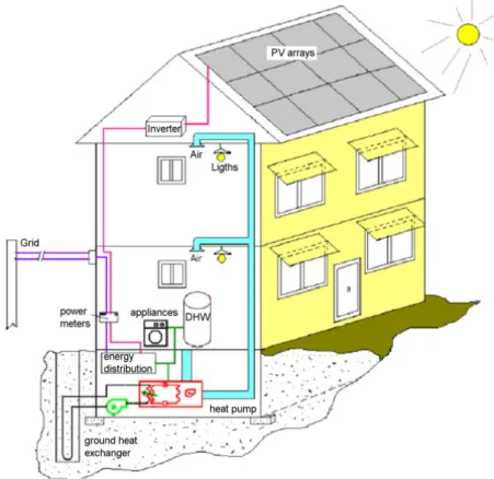
(17) in the industry expands the possibilities of the heat pump as a viable solution for energy efficiency increases in heat consumption systems. The operative range of temperatures for the HP technology finishes with temperatures up to 90ªC. The heat pump are the systems that allow to recover thermal energy from low temperature waste and convert it to high temperature heat (over 90ªC). This heat it’s demanded by the industry. [12]. Figure 4 Heat demand quality and quantity in European Markets by Industry. Source: Nellissen and Wolf, 2015. The Table 1 shows the operative temperatures and power ranges for the commercial solutions in heat pump energy recovery systems. Model – Company Oschner Heat Pumps Thermeco2 Hitachi Yutaki S80 Kobelco – HEM-HR90 Johnson Controls – Sabroe Heatpac MHI-Mitsubishi – ETW MAYEKAWA. Max. Temperature Produced Heat [ºC] 95 90 80 90. Max. Temperature Recovered Heat [ºC] 55 40 40 40. Thermal Power [kW] 60-850 45-1100 10-18 173-272. 90. 40. Up to 1800. 90. 50. 34-600. 35. 320-539. 83. Table 1 Commercial heat pump systems. Recent applications for heat recovery are related to the use of photovoltaic energy generation in buildings and industry. One big step in the implementation of heat pumps coupled with photovoltaic systems for water heating and climate control is with the zero net energy homes (ZNEH) implementation [13]. Those systems provide a hybrid system where technologies like photovoltaic generation and geothermal heat pumps work together to provide the building with water for the appliances and hot air for the climate system. See Figure 5.. 14.

(18) Figure 5 ZNEH schematic representation.. This type of systems could be escalated and implemented in public and commercial buildings to assist or substitute the traditional systems. In the industrial fields can be found a wide variety of applications suitable for incorporating the heat pump technology. As an example of the heat pump applications [14] in the industrial manufacturing activities see Table 2. Industry Petroleum refining and petrochemicals. Activity Distillation of petroleum and petrochemical products Inorganic salt manufacture including salt, sodium sulphate, sodium carbonate, boric acid. Chemicals. Treatment of process effluent. Heat recovery. Wood Products. Process. Heat-Pump type. Separation of propane/propylene, butene/butylene and ethane/ethylene. Mechanical Vapor Compression, Open Cycle. Concentration of product salt solutions. Mechanical Vapor Compression, Open Cycle. Concentration of waste streams to reduce hydraulic load on waste treatment facilities Compression of lowpressure waste steam or vapor for use as a heating medium. Pharmaceuticals. Process water heating. Pulp manufacturing. Concentration of black liquor. Paper manufacturing. Process water Heating. 15. Mechanical Vapor Compression, Open Cycle Mechanical Vapor Compression, Open Cycle Mechanical Compression, Closed Cycle Mechanical Vapor Compression, Open Cycle Mechanical Vapor Compression, Open Cycle.

(19) Paper manufacturing. Flash-steam recovery. Lumber manufacturing. Product drying. Manufacturing of alcohol Beer brewing. Food and beverage. Utilities. Concentration of waste liquids Concentration of waste beer. Wet corn milling/corn syrup manufacturing. Concentration of steep water and syrup. Sugar refining. Concentration of sugar solution. Dairy products. Concentration of milk of whey. Juice manufacturing. Juice concentration. General food-product manufacturing. Heating of process and cleaning water. Soft drink manufacturing. Concentration of effluent. Nuclear power Nuclear Power Manufacturing of drinking water Steam-stripping of waste water or process streams Electroplating industries. Concentration of radioactive waste Concentration of cooling tower blowdown Desalination of sea water Flash steam recovery Heating of process solutions Concentration of effluent Process and wash-water heating. Miscellaneous. Textiles. General manufacturing District heating. Space heating Concentration of dilute dope stream Process and wash-water heating Space heating Large-scale space heating. Removal of solvent from air streams Table 2 Heat Pump industrial applications. Solvent recovery. 16. Thermocompression, Open Cycle Mechanical Vapor Compression, Open Cycle Mechanical Vapor Compression, Open Cycle Mechanical Vapor Compression, Open Cycle Mechanical Vapor Compression, Open Cycle, Thermocompression, Open Cycle Mechanical Vapor Compression, Open Cycle Thermocompression, Open Cycle Mechanical Vapor Compression, Open Cycle Thermocompression, Open Cycle Mechanical Vapor Compression, Open Cycle Mechanical Compression, Open Cycle Mechanical Compression, Open Cycle Mechanical Vapor Compression, Open Cycle Mechanical Vapor Compression, Open Cycle Mechanical Vapor Compression, Open Cycle Thermocompression, Open Cycle Mechanical Compression, Closed Cycle Mechanical Vapor Compression, Open Cycle Mechanical Compression, Closed Cycle Mechanical Compression, Closed Cycle Mechanical Compression, Closed Cycle Mechanical Compression, Closed Cycle Mechanical Compression, Closed Cycle Mechanical Compression, Absorption, Closed Cycle Mechanical Compression, Open Cycle.

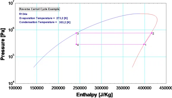
(20) 2.3.Thermodynamic cycle. The cycle corresponds to the vapor compression cycle, it stands as a cycle that allows to transfer heat using the expansion and compression of a fluid under certain conditions of pressure, temperature and flow. The heat pump developed is based on the ideal Vapor Compression Cycle, which correspond to the Reverse Carnot Cycle, see Diagram 1.. Diagram 1 Reverse Carnot Cycle example for R134a. The Reverse Carnot Cycle it’s the ideal cycle and it’s composed by 4 stages, as shown on the diagram 1 for R134a operating between an evaporation temperature of 273.15K and a condensation temperature of 303.15K: • • • •. Stage 1: from point 1 to point 2. Isentropic compression. Stage 2: from point 2 to point 3. Reversible isobaric heat change in which the working fluid is de-superheated and condensed. Stage 3: from point 3 to point 4. Isenthalpic expansion. Stage 4: from point 4 to point 1. Reversible isobaric heat change in which the working fluid is evaporated to is saturated vapor state.. This cycle is irreversible due to the isenthalpic expansion. The COP of the ideal cycle it’s defined with the operating temperatures following the equation: 𝐶𝐶𝐶𝐶𝐶𝐶𝐻𝐻𝐻𝐻,𝐶𝐶𝐶𝐶𝐶𝐶𝐶𝐶𝐶𝐶𝐶𝐶 =. 1 𝑇𝑇𝑒𝑒𝑒𝑒𝑒𝑒𝑒𝑒𝑒𝑒𝑒𝑒𝑒𝑒𝑒𝑒𝑒𝑒𝑒𝑒𝑒𝑒 1 − 𝑇𝑇 𝑐𝑐𝑐𝑐𝑐𝑐𝑐𝑐𝑐𝑐𝑐𝑐𝑐𝑐𝑐𝑐𝑐𝑐𝑐𝑐𝑐𝑐𝑐𝑐. Equation 1 Carnot COP with temperatures. In a real cycle, the COP is defined in the equation: 𝐶𝐶𝐶𝐶𝐶𝐶𝐻𝐻𝐻𝐻 =. 𝑄𝑄̇𝑐𝑐𝑐𝑐𝑐𝑐𝑐𝑐𝑐𝑐𝑐𝑐𝑐𝑐𝑐𝑐𝑐𝑐𝑐𝑐𝑐𝑐 𝑊𝑊̇𝑖𝑖𝑖𝑖 17. Equation 2 Heat Pump COP.

(21) And the power of the components is defined in the following equation: 𝑄𝑄̇ = 𝑚𝑚̇ · Δℎ. Equation 3 Thermal Power. Where the Qcondenser it’s the useful heat provided by the system and the Win it’s the total amount of energy consumed from the supply. [15] The vapor compression cycle it’s applied in refrigeration and in heat pumps, depending on which heat flow it’s the one used to design the system. There are several types and configurations of heat pumps depending on the components used, the simplest configuration allows to understand and study the general parameters and the correlations involved in the working process however it’s not the best configuration efficiency focused. The main components are always present but a variety of intercoolers, compressors, valves and heat exchangers are added to increase the overall COP of the system. The optimal configuration it’s based on the demands from the application and the suitability of the components and fluids to work and operate under those conditions. The first and simplest configuration of a heat pump with vapor compression cycle follows the diagram shown in Figure 6 and it’s composed by a compressor, a condenser, an expansion valve and an evaporator.. Figure 6 Simple configuration. This configuration it’s the basic iteration for the VCCHP, providing a cycle of work as shown on Diagram 1. This configuration allows to study the fluids under the ideal situation where the performance parameters would be ideal, based on the reverse Carnot cycle. In the real basic configuration, the performance parameters of the components are taken in account and the COP decreases. This configuration it’s limited by the working fluid, allowing only a correct state of operation in the design conditions, which makes a non-flexible system. 18.

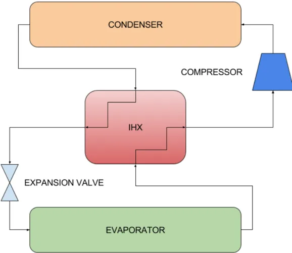
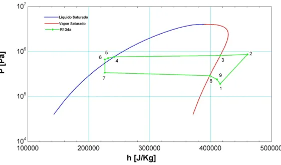
(22) Adding an Internal Heat Exchanger (IHX), as shown on Figure 7to the basic configuration allows to increase the real performance of the HP and allowing the system to adapt to minimal changes of the parameters of work. The IHX exchanges the heat between the superheated liquid fluid at the outlet of the condenser and the subcooled gas fluid at the outlet of the evaporator. This allows the compressor to work in the most efficient way and allowing the system to expand the range of working temperatures.. Figure 7 Internal Heat Exchanger configuration. The cycle for this configuration it’s like the reverse Carnot cycle diagram although incorporating more points to it. See Diagram 2 as an example of the cycle for the IHX configuration. The internal heat exchange occurs between points 5-6 and 9-1.. 19.

(23) Diagram 2 IHX cycle. The IHX configuration is common due to the flexibility and simplicity of components. It’s suitable for working with all the refrigerants and doesn’t present points with complex mixtures of gas and liquid. This configuration it’s the common base for the HP systems found in the market. The next step in the development of configurations is allowing to operate in a wider range of temperatures and pressures. This is accomplished by the addition of compressors, view Figure 8, or coupling multiple individual HP systems, view Figure 9. These configurations are complex systems, suitable for working in low temperature environments and with fluids working in trans-critical conditions. [16–20]. Figure 8 Two-Stage compressor configuration. 20.

(24) Figure 9 Cascade configuration. The research in heat pumps is focusing on the develop of suitable cascade systems [16–18] , more efficient and capable to operate with a variety of fluids with low GWP. In this work, the configuration chosen for modelling is the Internal Heat Exchanger configuration as shown on Figure 7.. 2.4.Main Components. The vapor compression cycle heat pump is composed by three types of principal components; compressor, expansion device and heat exchangers. Those components present different geometries and dispositions depending on the working fluid of the system and the working conditions. Each system is rather unique and must be dimensioned and designed for each application, including in most cases even the components. Other components act as safety devices and helps to monitor the correct operation of the heat pump providing a controlled stop in case of malfunction. Some of these components are often reflected in the legislation for refrigeration and heat pumps installation, especially in high pressure systems or high temperature systems due to the danger that represents for the workers and the surroundings.. 2.4.1. Compressor There are several different types of compressors, differing in performance capabilities and working principles. In the following figures, the common types of compressors are exemplified.. 21.

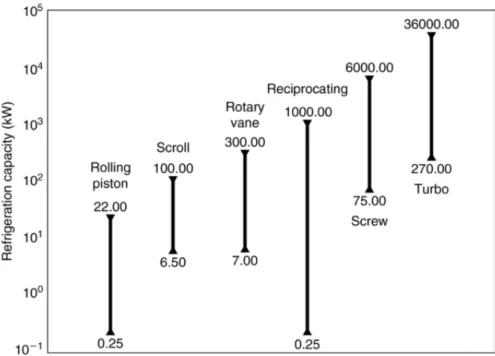
(25) Figure 10 Reciprocating Compressor. Figure 11 Scroll Compressor. Figure 12 Screw Compressor. The main types of compressors and their range of operation are shown in Figure 13 [21].. 22.

(26) Figure 13 Compressor types and range of operation.. •. •. Positive Displacement o Reciprocating o Rotary  Vane  Scroll  Rolling piston  Screw Dynamic o Ejector/jet o Turbo  Centrifugal  Axial. The compressors are the most important component of the system. Provides the work needed to operate and are suitable of malfunctioning and eventually breakdown if they’re forced to work in conditions out of the range. It’s also the component which requires more attention from the maintenance point of view, most of the compressors need oil or other lubricant fluids to operate properly and provide the best performance. The correct selection of the compressor is a main goal to provide the best COP by the heat pump or refrigerator. This selection should be made analysing and comparing the options within the range of work and taking account of the characteristics of the working fluid used in the system. Some fluids are suitable to work with oils and lubricants but others present chemical reactions with these lubricants under certain work conditions.. 23.

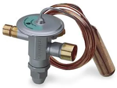
(27) 2.4.2. Expansion device. Figure 14 Expansion Valve. The expansion device acts as an actuator before the fluid enters the evaporation zone triggering this phase change. Is located in between the high-pressure condensation zone and the lowpressure evaporation zone. Usually the expansion device is a valve, which is regulated to operate at the designated pressure in the cycle. By the variation of the regulation for the trigger pressure of the valve variable temperatures of evaporation are possible always assuring the integrity of the rest of the components in the system. There are other types of expansion devices such as capillary tubes but doesn’t allow any type of regulation. The newest technology in valves allow to control electronically the discharge pressure so the behaviour of the system can be changed to accommodate to different working parameters without the need to replace parts. [22] In reversible configurations such as the ones found in climate control three-way valves are found, which by switching positions allow the flow to change direction so the system can work as a heat pump or as a refrigeration unit. This only work for certain fluids and components but it’s a common configuration that can be found in domestic installations where the range of temperatures are low. The expansion valves must assure one direction of flow in the system so there is not fluid returning to the compressor when the system is running, and must be closed, either by itself or by another solenoid valve, when the system is stopped.. 2.4.3. Heat exchanger The heat exchanger is the device where the transmission of heat with the secondary fluid happens, as a minimum there’ll be two heat exchangers, one as a condenser and one as an evaporator. They must assure the complete phase-change inside them, so de geometry and dimensions of each one must be precisely defined in the design. The correct transmission of heat is the final goal of the Heat Pump and the condenser is the exchanger that provides that heat.. 24.

(28) Figure 15 Heat Exchangers: shell and tube (left) and plate exchangers (right).. Depending on the configuration several heat exchangers with different geometries and parameters could be found on a Heat Pump. The simplest exchanger is the straight concentric tube, Figure 16, where one fluid flows on the outer tube and the other flows in the inner tube, either in the same direction or opposite, and where the heat exchange occurs in the cylindrical area defined by the inner tube.. Figure 16 Diagram of a Concentric Cylindrical Exchanger. Another exchanger configuration includes plates and helicoidal geometries to increase the area of exchange to the maximum without losing too much pressure. The limit parameters for exchangers are the velocity of the fluid, the heat transfer and the pressure drop. Those three parameters determine the geometry and the behaviour of the exchanger and there are several mathematical methods and correlations to relate one to another depending on the geometry and the characteristics of the flow inside the exchanger. The geometry of this exchangers will determine the cost of the exchangers, varying in large amounts depending on the complexity and materials used. In the specific application for evaporator and condenser the exchanger must be larger than the optimal designed for guarantee a superheat or Subcooling at the end of the phase change and thus avoid possible malfunctions.. 25.

(29) 2.4.4. Safety and control devices In every heat pump system must be a series of safety and control devices and subsystems to guarantee the perfect performance and prevent critical malfunctioning of the system. Those devices are defined by specific legislation depending on the final application of the heat pump system and the parameters of work of it, e.g. pressure, temperature, flammability of the working fluid, toxicity, possible presence of explosive atmospheres; and this legislation varies in different countries. These regulations should be taken in account in the selection of the components for the system. The control devices don’t affect the system at any point, they only provide information and data about the working parameters of the system to check the correct functioning. As control devices, we can find from thermometers and manometers in the simplest configurations and systems, up to electronic flowmeters and PLCs monitoring and transmitting the data of the system.. Figure 17 Safety Devices. In the other hand, the safety devices did affect the system, e.g. shutting down the system or releasing pressure from it. They only enter on the operation as an ultimate measure and commonly trigger an irreversible action after which maintenance checking and replacement of parts and fluids must occur. The safety devices are e.g. high-pressure release valves and lowpressure release valves, fluid detectors to avoid recirculation of fluid or lubricant, temperature sensors and solenoid valves to shut down the system. This kind of devices must be configured and placed with the correct criteria to allow the system to work correctly and to protect and reduce the danger in case of an accident.. 2.5.Working fluids. The working fluids or refrigerants are the fluids inside the system. The refrigerants used in the heat pump and refrigeration systems has changed drastically through the years although some of them persist as an option even today and are object of development and research. Nowadays the refrigerants must have some characteristics to be allowed for use referring to the ODP and the GWP parameters. It also must fulfil a series of requirements such as non-toxic or nonflammable depending on the system’s application. The nomenclature applied to the refrigerants it’s settled by the American Society of Heating, Refrigerating and Air-Conditioning Engineers (ASHRAE). This nomenclature provide a standard to identify refrigerants, its nature and some of the characteristics, providing also safety information. [23] 26.

(30) The classification of the fluids is based on a system of families taking account of the nature and the global characteristics, although other classifications are made depending on the criteria selected, e.g. ODP or GWP. The general classification for refrigerants depending on the type of fluid based on the behaviour is: • •. Pure Mixture o Zeotropic o Azeotropic o Near-azeotropic o Non-azeotropic. Over the years new parameters define the fluids e.g. safety, durability, ODP or GWP, which determine the usage of the fluids. In Figure 18 a timeline is displayed showing the main families and the main events, remarking the use of natural fluids or hydrocarbons for industrial refrigeration since the early ages of the 19th century, what has been called First Generation Refrigerants. Until 1930, when Thomas Midgley developed the chlorofluorocarbons (CFCs), the refrigeration technology and heat pump was limited only to industry application due to the risk and cost of the systems implemented but with Midgley developments the refrigeration expanded to domestic use thanks to the stability and characteristics of the CFCs and HCFCs, allowing smaller components and working pressures. The evolution of the industrial refrigeration continued using natural refrigerants due to the cost of the new CFCs and HCFCs for big installations, natural refrigerants e.g. Ammonia, were much cheaper than other ones like R-22. Due to the research conducted by Molina and Rowland in the 70s decade, regarding the ozone layer depletion by the CFCs, the Montreal Protocol was pronounced and signed in 1987 regulating the usage of CFCs and HCFCs which have a high ODP coefficient. Few years later the focus was turned to the climate change potential of the refrigerants, and the Kyoto Protocol followed the Montreal Protocol regulating the usage of refrigerants with high GWP. Nowadays CFCs, HCFCs and HFCs refrigerants are in disuse both because of legislation which limits and bans the usage and because of cost of operation. The development and research has returned to natural refrigerants, HFOs, HCs and mixtures. With the development of new configurations and better equipment a performance previously unreachable has been achieved, allowing the usage of them in applications dismissed in the past. [24,25]. 27.

(31) Figure 18 Timeline of refrigerants development. In addition to the GWP and ODP values, ASHRAE classifies the refrigerants with a Safety Group [26] based on this table: Higher Flammability Lower Flammability No Flame Propagation. A3 A2 A2L* A1 Lower toxicity. Safety Group. Table 3 Safety Group clasiffication. B3 B2 B2L* B1 Higher toxicity. *A2L and B2L are lower flammability refrigerants with a maximum burning velocity of ≤ 10cm/s. The values of GWP are stated in the F-Gas regulation [4] and the ODP on the Montreal Protocol [1]. The range of usage for the refrigerants it’s defined by the behaviour under certain conditions of temperature and pressure. In Diagram 3 the curves for several common refrigerants are displayed comparing the different range of temperatures and behaviour for different refrigerants.. 28.

(32) ASHRAE Designation. R134a R1234yf R1234ze R12 R22 R407 R404A R410A R245fa R744 R717 R718. Chemical Name. Family. 1,1,1,2-tetrafluoroethane 2,3,3,3-tetrafluoro-1propene trans-1,3,3,3-tetrafluoro-1propene dichlorodifluoromethane 12B1 chlorodifluoromethane trifluoromethane R-32/125/134a (23.0/25.0/52.0)o R-125/143a/134a (44.0/52.0/4.0)f R-32/125 (50.0/50.0) 1,1,1,3,3pentafluoropropane Carbon Dioxide Ammonia Water. Chemical Formula. Critical Pressure [MPa]. Critical Temperature [K]. GWP100 [27]. ASHRAE Safety Group [Table 3]. OPD [27]. HFC. CH2FCF3. 4.059. 374.21. 1430. 0. A1. HFO. CF3CF=CH2. 3.382. 367.85. 4. 0. A2L. HFO. CF3CH=CHF. 3.636. 382.52. 6. 0. A2L. CFC. CCl2F2. 4.136. 385.12. 10900. 1. A1. HCFC. CHClF2. 4.99. 369.3. 1810. 0.055. A1. HFC. Blend. 4.632. 359.345. 1774. 0. A1. HFC. Blend. 3.735. 345.27. 3922. 0. A1. HFC. Blend. 4.901. 344.494. 2088. 0. A1. HFC. CHF2CH2CF3. 3.651. 427.01. 2. Natural Natural Natural. CO2 NH3 H2O. 7.377 11.333 22.064. 304.1282 405.4 647.096. 1000 0 0. Table 4 Fluids properties and information.. B1 1 0 0. PT chart 10000. Saturation Pressure [Pa]. R134a R407C. 1000. R404A R410A R245fa. 100. R12 R22 R1234yf. 10. R1234zeE R744 R717. 1. 230. 280. 330. 380. Saturation temperature [K] Diagram 3 PT chart for several refrigerants at saturation. Data Source: Coolprop. 29. R718. A1 B2 A1.

(33) The work focuses on three different types of refrigerants: ASHRAE Designation. R134a. R1234yf. R1234zeE. Chemical Name. 1,1,1,2-tetrafluoroethane. 2,3,3,3-tetrafluoro-1-propene. trans-1,3,3,3tetrafluoro-1propene. Chemical Formula. CH2FCF3. CF3CF=CH2. CF3CH=CHF. Critical Pressure [MPa]. 4.05928. 3.3822. 3.63625. Critical Temperature [K]. 374.21. 367.85. 382.52. GWP100 [27]. 1430. 4. 6. OPD [27]. 0. 0. 0. Safety Group. A1. A2L. A2L. Slope. Isentropic. Isentropic. Isentropic. Boiling Temperature at atmospheric pressure [K]. 247.076. 243,665. 254,182. Cp at Boiling temperature [KJ/Kg]. 196.22. 198.061. 210.759. 0.883. 0.892. 0.665. 2.625. 2.512. 2.001. 154.365. 179.431. 119.704. 929.386. 810.284. 933.574. 2.059. 2.218. 1.789. 2.003. 2.348. 1.54. Evaporation pressure at 35ºC [Mpa] Condesation pressure at 80ºC [Mpa] saturated gas density at 80ºC [Kg/m3] Saturated liquid density at 80ºC [Kg/m3] Saturated liquid specific heat at 80ºC [KJ/Kg·K] Saturated Gas specific heat at 80ºC [KJ/Kg·K]. Table 5 R134a/R1234yf/R1234zeE Data. Values for Critical Pressure and Critical Temperature from CoolProp Fluids properties, Pure and Pseudo-Pure fluid properties.. 30.

(34) PT chart: CFC - HFC - HFO evolution. Saturation Pressure [KPa]. 3000. 300. 30. 230. 250. 270. 290. 310. 330. 350. Saturation Temperature [K] R12. R134a. R1234zeE. R1234yf. Diagram 4 R12/R134a/R1234ze(E)/R1234yf Data Source: Coolprop. P-h. Pressure [MPa]. 10. 1. 0,1. 0,01. 0. 50. 100. 150. 200. 250. 300. 350. 400. 450. 500. Enthalpy [KJ/Kg] R134a. R1234yf. R1234zeE. Diagram 5 Pressure-Enthalpy graph for R134a/R1234yf/R1234zeE Data Source: Coolprop. The R134a is a common refrigerant from the HFC family used in a lot of different applications in low and mid-temperature applications due to is range of operation, which comprehends temperatures between -30 to +20ºC [28] for evaporation. It was introduced in the industry of refrigeration and heat pumps in the early 1990s as a replacement for R12 (CFC) due to its similar characteristics and the capacity to work under the 31.

(35) same conditions. It has insignificant ODP but a medium level GWP, which is taxed by the most recent legislation. The replacement for R134a has been under development with the R1234yf and R1234ze, both from the HFO family of refrigerants. In Diagram 4 is represented the similar behaviour between these refrigerants. Several researches has been published in the field e.g the work conducted by Nawaz, Shen, Elatar, Baxter and Abdelaziz on the residential water heater application [29].. 3. Model The model has been developed in Engineering Equation Solver [6] with the CoolProp Database [7] as a complement to obtain the fluid data. It’s an iterative model which resolves point to point the cycle and calculates the dimensions for the optimal exchangers to perform at the given range of temperatures with the selected fluid. The model it’s based on the Reverse Carnot Cycle model and evolves into the IHX configuration model as shown on Figure 7, taking account of the performance parameters from the compressor and the pressure losses in the exchangers. In Figure 19 is represented the evolution process of the model.. Figure 19 Model evolution. 3.1.System Description. The model scheme corresponds to the Figure 20.. Figure 20 Model Scheme. 32.

(36) Steps resolved in the model: A. Point 1-2: Compression stage. Refrigerant in gas phase. B. Point 2-3: Heat exchange from the refrigerant to the secondary fluid of the heat application without phase change. Refrigerant in gas phase. C. Point 3-4: Condensation stage. Heat exchange from the refrigerant to the secondary fluid of the heat application with phase change. D. Point 4-5: Subcooling stage. Heat exchange from the refrigerant to the secondary fluid of the heat application without phase change. Refrigerant in liquid phase. E. Point 5-6: Internal Heat Exchanger. Heat exchange from the refrigerant in liquid phase to the refrigerant in gas phase. F. Point 6-7: Expansion stage. Pressure drop of the refrigerant triggering the phase change. G. Point 7-8: Evaporation stage. Heat exchange from the secondary fluid of the heat source to the refrigerant in phase change. H. Point 8-9: Superheat stage. Heat exchange from the secondary fluid in the heat source to the refrigerant. Refrigerant in gas phase. I. Point 9-1: Internal Heat Exchange. Heat exchange from the refrigerant in liquid phase to the refrigerant in gas phase.. 3.2.Starting hypotheses. The hypotheses considered in the process of modelling the system are: • • • • •. The flow in the single-phase zones is turbulent. There is no pressure loss in the pipes of the system between components. The exchangers have smooth surfaces in the tubes. Water has been selected as the secondary fluid, both for the heat source and for the application. The expansion in the expansion valve is isenthalpic without heat transfer.. 3.3.Components modelling. For the numerical resolution of the system some parameters must be determined as a starting point. The parameters are those related to the components materials and performances. The components are modelled from the initial data given to the program. There are some parameters affecting the components modelling which are external and not directly related to the components. Those parameters are: Parameter Copper thermal conductivit Secondary fluids pressure Liquid limit velocity Gas limit velocity Exchangers wall thickness. 385 W/m·K 0.2 MPa 1 m/s 5 m/s 1 mm. Table 6 System modelling parameters. 33. Value.

(37) 3.3.1. Compressor For the modelling of the compressor the parameters settled are the performance parameters. Parameter Isentropic performance – ηis Volumetric performance – ηvol Global performance – ηglob. Value. 0.8 0.85 0.75. Table 7 Compressor modelling parameters. The compressor power input affects the COP of the system, which is the global performance parameter. The COP parameter is defined in the Equation 4, which it’s an adaptation of Equation 2 to the model. 𝐶𝐶𝐶𝐶𝐶𝐶 =. 𝑄𝑄̇𝑐𝑐𝑐𝑐𝑐𝑐𝑐𝑐𝑐𝑐𝑐𝑐𝑐𝑐𝑐𝑐𝑐𝑐 𝑊𝑊̇𝑐𝑐𝑐𝑐𝑐𝑐𝑐𝑐𝑐𝑐𝑐𝑐𝑐𝑐𝑐𝑐𝑐𝑐𝑐𝑐. Equation 4 Model COP. For calculating the compressor power, the equation used is the Equation 5. 𝑊𝑊̇𝑐𝑐𝑐𝑐𝑐𝑐𝑐𝑐𝑐𝑐𝑐𝑐𝑐𝑐𝑐𝑐𝑐𝑐𝑐𝑐 =. 𝑚𝑚̇ · (ℎ[2] − ℎ[1]) 𝜂𝜂𝑔𝑔𝑔𝑔𝑔𝑔𝑔𝑔. Equation 5 Compressor Power. The volumetric capacity of the compressor, affected by the volumetric performance parameter, is defined in Equation 6. 𝑉𝑉𝑐𝑐𝑐𝑐𝑐𝑐𝑐𝑐𝑐𝑐𝑐𝑐𝑐𝑐𝑐𝑐𝑐𝑐𝑐𝑐 =. 𝑚𝑚̇ 𝜌𝜌[1] · 𝜂𝜂𝑣𝑣𝑣𝑣𝑣𝑣. Equation 6 Volumetric Capacity of the compressor. And finally, the isentropic performance parameter interacts with the system as shown in Equation 7, varying the enthalpy on the outlet from is ideal point, h[2]s. ℎ[2] =. ℎ[2]𝑠𝑠 − ℎ[1] + ℎ[1] 𝜂𝜂𝑖𝑖𝑖𝑖. Equation 7 Isentropic performance interaction. 3.3.2. Expansion Device The expansion device is selected in the model by the mass flow of the system. Doesn’t affect the system in the performance parameters due to its function, acting as a trigger for the evaporation of the fluid. There is no heat loss or work involved in is operation.. 3.3.3. Heat Exchangers The heat exchangers are the key components of the system. There’s three of them and each one must be treated separately due to the different thermodynamic processes taking place inside of them. The common values for the exchangers are those related to the pressure drop and they’re mathematically formulated as shown on the following equations. The heat transfers are calculated using the following equations and schemes: 34.

(38) 𝑄𝑄̇ = 𝑈𝑈 · 𝐴𝐴 · Δ𝑇𝑇𝐿𝐿𝐿𝐿. Equation 8 Heat Transfer between fluids. Where the logarithmic mean temperature average comes defined in the Equation 9 Δ𝑇𝑇𝐿𝐿𝐿𝐿 =. Δ𝑇𝑇𝐴𝐴 − Δ𝑇𝑇𝐵𝐵 Δ𝑇𝑇 𝑙𝑙𝑙𝑙 � 𝐴𝐴 � Δ𝑇𝑇𝐵𝐵. Equation 9 Logarithmic Mean Temperature Average. Δ𝑇𝑇𝐴𝐴 = 𝑇𝑇𝑖𝑖𝑖𝑖,1 − 𝑇𝑇𝑜𝑜𝑜𝑜𝑜𝑜,2. Equation 10 Temperature Difference A. Δ𝑇𝑇𝐵𝐵 = 𝑇𝑇𝑜𝑜𝑜𝑜𝑜𝑜,1 − 𝑇𝑇𝑖𝑖𝑖𝑖,2. Equation 11 Temperature Difference B. All the exchangers have a concentric tube configuration, due to the geometrical simplicity and the possibility to extrapolate the results to other heat exchanger configurations. The basic parameters for the exchangers geometry are the radius (R1, R2 and R3) as shown on Figure 20 and the length. The temperature gradient inside the exchanger correspond to the scheme shown on Figure 22. This scheme will vary depending on the phase of the fluids and the heat transfer coefficient.. Figure 21 Concentric Heat Exchanger Geometry. 35.

(39) Figure 22 Heat Exchanger Temperature scheme. The global heat transfer coefficient of the exchanger comes defined by the following equations affected by the different thermal resistances inside the exchanger, due to multiple heat transfer methods (conduction and convection). 𝑈𝑈 =. 1 𝐴𝐴 · 𝑅𝑅𝑇𝑇. 𝑅𝑅𝑇𝑇,𝑐𝑐𝑐𝑐𝑐𝑐𝑐𝑐𝑐𝑐𝑐𝑐𝑐𝑐𝑐𝑐𝑐𝑐𝑐𝑐 = 𝑅𝑅𝑇𝑇,𝑐𝑐𝑐𝑐𝑐𝑐𝑐𝑐𝑐𝑐𝑐𝑐𝑐𝑐𝑐𝑐𝑐𝑐𝑐𝑐 =. Equation 12 Global Heat Transfer Coefficient. 1. 𝐴𝐴 · 𝛼𝛼𝑐𝑐𝑐𝑐𝑐𝑐𝑐𝑐𝑐𝑐𝑐𝑐𝑐𝑐𝑐𝑐𝑐𝑐𝑐𝑐. Equation 13 Convection Thermal Resistance. 𝑟𝑟 𝑙𝑙𝑙𝑙� 𝑒𝑒�𝑟𝑟𝑖𝑖 �. 2 · 𝜋𝜋 · 𝐿𝐿 · 𝐾𝐾𝑚𝑚𝑚𝑚𝑚𝑚𝑚𝑚𝑚𝑚𝑚𝑚𝑚𝑚𝑚𝑚. Equation 14 Conduction Thermal Resistance. 𝑅𝑅𝑇𝑇 = 𝑅𝑅𝑇𝑇,𝑐𝑐𝑐𝑐𝑐𝑐𝑐𝑐𝑐𝑐𝑐𝑐𝑐𝑐𝑐𝑐𝑐𝑐𝑐𝑐 + 𝑅𝑅𝑇𝑇,𝑐𝑐𝑐𝑐𝑐𝑐𝑐𝑐𝑐𝑐𝑐𝑐𝑐𝑐𝑐𝑐𝑐𝑐𝑐𝑐. Equation 15 Global Thermal Resistance. With the equations defined the relation between the global heat transfer coefficient, the heat transfer coefficient of each fluid and the geometric parameters of the exchanger are related in an equation, as shown on Equation 16. 𝑈𝑈 · 𝐴𝐴 =. 2 · 𝜋𝜋 · 𝐿𝐿. 𝑅𝑅2 𝑙𝑙𝑙𝑙 �𝑅𝑅1� 1 1 𝐾𝐾𝑚𝑚𝑚𝑚𝑚𝑚𝑚𝑚𝑚𝑚𝑚𝑚𝑚𝑚𝑚𝑚 + 𝛼𝛼𝑜𝑜𝑜𝑜𝑜𝑜 · 𝑅𝑅2 + 𝛼𝛼𝑖𝑖𝑖𝑖 · 𝑅𝑅1. Equation 16 Relationship between length and heat transfer. Those equations are common for all the exchangers although the heat transfer coefficient for the fluids vary depending if the phase is liquid, gas or if it’s changing. In a single exchanger may occur to find the three possible phases of a fluid. In those cases, the mathematical model of the exchanger must face each stage separately.. 36.

(40) Single-phased stages For the analysis of the stages the Reynolds, Prandtl and Nusselt numbers are required, and those numbers vary with the phase of the fluid and the geometry of the conducts. The Reynolds number is defined in the Equation 17. 𝑅𝑅𝑅𝑅 =. 𝜌𝜌 · 𝜐𝜐 · 𝐷𝐷 𝜇𝜇. Equation 17 Reynolds Number. The flow pattern it’s defined by the Reynolds number using the following criteria: • • •. Re < 2300 – Laminar Flow 2300 < Re < 10000 – Transition 10000 < Re – Turbulent. The Prandtl number is defined in the Equation 18. 𝑃𝑃𝑃𝑃 = 𝐶𝐶𝑝𝑝 ·. 𝜇𝜇 𝑘𝑘𝑓𝑓. Equation 18 Prandtl Number. The heat transfer coefficient in single phase is defined in the Equation 19. 𝛼𝛼𝑐𝑐𝑐𝑐𝑐𝑐𝑐𝑐𝑐𝑐𝑐𝑐𝑐𝑐𝑐𝑐𝑐𝑐𝑐𝑐 = 𝑁𝑁𝑁𝑁 ·. 𝑘𝑘𝑓𝑓 𝐷𝐷. Equation 19 Heat Transfer Coefficient for single phase. For the calculation of the Nusselt number in single phase this project uses the Gnielinski correlation [34] defined in the Equation 20. 𝑓𝑓 · (𝑅𝑅𝑅𝑅 − 1000) · 𝑃𝑃𝑃𝑃 8 𝑁𝑁𝑁𝑁 = 1 2 𝑓𝑓 �2 1 + 12.7 · �8� · �𝑃𝑃𝑃𝑃 �3 − 1�. Equation 20 Gnielinski correlation for Nusselt number. 𝑓𝑓 = (0.79 · ln(𝑅𝑅𝑅𝑅) − 1.64)−2 The conditions of application for the Gnielinski correlation are: • •. 0.5 < Pr and 3000 < Re < 106 104 < Re < 5·106. 37. Equation 21 Friction Factor.

(41) For the pressure loss in single phase this project uses the Darcy-Weisbach correlation. This pressure loss is due to the friction between the fluid and the surface of the exchanger in contact with it. The Equation 22 and the Equation 21 defines the Darcy-Weisbach correlation and the friction factor respectively. Δ𝑃𝑃𝑓𝑓𝑓𝑓𝑓𝑓𝑓𝑓𝑓𝑓𝑓𝑓𝑓𝑓𝑓𝑓 = 𝑓𝑓 ·. 𝐿𝐿 𝜌𝜌 · 𝑢𝑢2 · 2 𝐷𝐷. Equation 22 Darcy-Weisbach correlation. Internal Heat Exchanger The internal heat exchanger between the points 5-6 and 9-1 in the system only has fluid in single phase. Between 5-6 the fluid is in liquid phase and between the points 9-1 the fluid is in gas phase. The heat flow of the internal heat exchanger is: ̇ = 𝑚𝑚̇ · (ℎ[1] − ℎ[9]) 𝑄𝑄𝐼𝐼𝐼𝐼𝐼𝐼. Equation 23 IHX power. The liquid fluid from the condenser (points 5 to 6) will be in the inner tube and the gas fluid from the evaporator (points 9 to 1) will be in the outer tube. The geometry calculation is conducted with the velocity parameters for liquid and gas. The internal heat exchanger has an efficiency set at 0.85 for the reference point. This efficiency affects and modifies the power transmission as defined by Equation 24 𝜀𝜀𝐼𝐼𝐼𝐼𝐼𝐼 =. ℎ[1] − ℎ[9] ℎ𝑚𝑚𝑚𝑚𝑚𝑚 − ℎ[9]. Equation 24 IHX efficiency parameter. Evaporator The evaporator is the heat exchanger where the phase change from fluid to gas and the superheat stage takes place. There’s two stages to calculate, the phase change stage and the single-phase stage. See Figure 23.. 38.

(42) Figure 23 Evaporator stages. The parameters defined for the evaporator calculation are: Parameter ΔT – temperature increment TG – temperature gap SH – Super Heat temperature Tin,1 – secondary fluid inlet temperature Q_evaporator – Evaporator power. 10 ºC 5 ºC 10 ºC 290 K 10000 W or 10 kW. Value. Table 8 Evaporator modelling parameters. The evaporator power is defined in Equation 25, with this equation the mass flow of the system is defined and calculated as a relation with the evaporator power needed in the application. 𝑄𝑄̇𝑒𝑒𝑒𝑒𝑒𝑒𝑒𝑒𝑒𝑒𝑒𝑒𝑒𝑒𝑒𝑒𝑒𝑒𝑒𝑒 = 𝑚𝑚̇ · (ℎ[9] − ℎ[7]). Equation 25 Evaporator Power. The calculation for the single-phase stage of the evaporator is conducted with the same equations as in the IHX. The phase change stage of the evaporator is calculated using the Gungor-Winterton correlation [35] (Equation 28) and the Pierre correlation modified [36] (Equation 37) for the pressure loss due to the phase change. The total length of the exchanger and drop pressure would be the combination of the lengths and pressure drops from its stages.. 39.