INSTITUTO TECNOLÓGICO DE COSTA RICA ESCUELA DE QUÍMICA
CARRERA DE INGENIERÍA AMBIENTAL
Final Graduation Project to qualify for the University Degree of Environmental Engineering
“Development of a modelling tool for simulating electricity demand and on site Photovoltaics power production in high time resolution: Applications in Costa Rica.”
"Desarrollo de una herramienta de modelado con tiempo en alta resolución para simular la demanda energética y la producción de energía fotovoltaica in situ: Aplicaciones en Costa Rica."
Sophia Ruiz Vásquez
III
ACKNOWLEDGMENTS
I would like to thank my advisor Dr.Vicky Cheng and MSc. Anahi Molar Cruz from the Technishe Universität München, for all the immense knowledge, tools, support and advise that they constantly gave me throughout my research. I also thank all the professors of the Environmental Engineer major and my tutor Ing. Carlos Roldán Villalobos for sharing their knowledge with me.
I would like to express my most sincere gratefulness to the organization Bayerisches Hochsculzentrum für Lateinamerika (BAYLAT), for the honour of being selected as a scholarship holder which allowed me to performed part of this project in the city of Munich, Germany.
To the Enertiva Company, which gave me access to fundamental information that allowed me to conduct this project.
I want to express an enormously thank to all my friends that have given me their support and positivity making my life joyful. Particularly to my university friends, for the long but great projects, adventures and knowledge we shared together.
IV
TABLE OF CONTENTS
List of figures VI
List of acronyms and abbreviations IX
List of symbols XI
2.1.2. Renewable Energy Potential Use 5
2.1.2.1. Solar power potential: Irradiation data 6
2.1.3. Greenhouse Gas Emissions (GGE) 7
2.1.4. Energy demand 8
2.2. Dwelling energy demand 9
2.2.1. Modelling household energy demand 10
2.2.1.1. Top-down modelling 12
2.2.1.2. Bottom-up modelling 12
2.3. Bottom-up model of the Centre for Renewable Energy Systems Technology of
Loughborough University 13
2.3.1. Occupancy 15
2.3.2. Switch on events 16
2.3.3. Lighting model 16
2.4. PV power production 18
2.4.1. Generalities and components 18
2.4.2. Categories 20
2.4.3. Power production 20
2.4.4. Simulations of PV power production 21
V
3. Methodology 23
3.1. Domestic energy demand model 23
3.1.1. Occupancy 23
3.2. PV power production on-site model 27
3.2.1. Weather data 30
3.2.2. Validation of the model 31
3.3. Energy matching indexes 33
3.3.1. Error in the matching results 34
4. Results and Discussion 36
4.1. Validating the modelling tool: Dwelling energy demand 36 4.2. Validation of the model: PV on site power generation 40
4.3. Matching indexes 48
Appendix 1: Visualization of the PV on-site power production in different sky conditions
for extacting daily profiles from the month of March. 69
Appendix 2: High resolution domestic energy demand model 71 Appendix 3: High resolution PV power on-site production model 71
8. Annexs 72
Annex 1: Allocation sample of the appliances 73
Annex 2: Monitoring devices of Enlighten 75
VI
LIST OF FIGURES
Figure 2.1. Total secondary energy consumption structure of the year 2013. 3
Figure 2.2 Costa Rica´s energy generation in 2015. 5
Figure 2.3. National Electric System Contributions of the year 2012. 7 Figure 2.4. History and forecast of the net electricity generation. 8 Figure 2.5. Different sectors share of electricity consumption in the year 2014. 9 Figure 2.6. Natural logarithmic curve used to estimate relative weightings. 18
Figure 2.7. Typical PV system layouts with one array. 19
Figure 3.1. Localization of the house in study with the coordinates 9.944842, -84.034901. 26 Figure 3.2. Localization of the house in study with the coordinates 9.919044, -84.126521.
27
Figure 3.3 Diagram of the Enphase working system. 32
Figure 3.4. Matching indexes representation. 34
Figure 4.1. First house measured and model data annual profile. 37 Figure 4.2. Different simulated daily profiles of a weekday of January. 38 Figure 4.3. Second house measured and model data annual profile. 39 Figure 4.4. Annual energy produced by a PV installation of 6 micro inverters. 42 Figure 4.5. On-site electricity profile generated with clear sky conditions. 43 Figure 4.6. On-site electricity profile generated with cloudy sky conditions. 43 Figure 4.7. Annual energy produced by PV installation of 17 micro inverters. 45 Figure 4.8. On-site electricity profile generated with clear sky conditions 46 Figure 4.9. Annual energy produced by PV installation of 28 micro inverters. 47 Figure 4.10. Dry season day with clear sky on-site electricity generation profile. 49 Figure 4.11. Dry season day with partially cloudy sky on-site electricity generation profile.
VII Figure 4.16. Electricity consumption profile, L(t) and on-site generation profile, G(t) of a
sample in a dry season day with clear sky. 54
Figure 4.17. Electricity consumption profile, L(t) and on-site generation profile, G(t) of a
sample in a dry season day with partially cloudy sky. 54
Figure 4.18. Electricity consumption profile, L (t) and on-site generation profile, G(t) of a
sample in a dry season day with cloudy sky. 55
VIII
LIST OF TABLES
Table 2.1. Environmental indicators of Costa Rica, 4
Table 2.2. Energetic Local Potential of the year 2012. 6
Table 2.3. Categorization of appliances based on the demand share in Europe. 10
Table 2.4 Block set of appliances used in the model 13
Table 3.1 Categorization of the equations and values for standard PV test 29 Table 4.1. Data obtained from the simulation of the model and real data of the first house in
study. 36
Table 4.2. Data obtained from the simulation of the model and real data of the second house
in study. 38
Table 4.3. Values used in the simulation of the PV power generation on-site model. 41 Table 4.5. Data obtained and simulated of a system with 17 micro inverters. 44 Table 4.6. Data obtained and simulated of a system with 28 micro inverters. 46 Table 4.7. eOEM and eOEF error results in different sky conditions of the month of March.
52 Table 4.8. OEM and OEF results in different sky conditions of a weekday in the month of
March 56
Table 4.9. Hourly resolution between the PV power on-site production and the electricity
demand. 57
Table 4.10. Minimum minute resolution between the PV power on-site production and the
electricity demand. 57
Table An.1.1. Sample of the model’s input data based on the characteristics of the first
dwelling in study. 73
Table An.1.2. Sample of the model’s input data based on the characteristics of the second
IX
LIST OF ACRONYMS AND ABBREVIATIONS
CFL Compact Fluorescent Light
CNFL Compañia Nacional de Fuerza y Luz
EESC Energy Efficient and Smart City
GGE Green Gas Emissions
GLS General Lighting Service
ICE Instituto Nacional de Energía
LED Lighting Emitting Diode
LIA Lighting Industry Association
PAR Parabolic Aluminized Reflector
SPD Surge Protection Devices
XI
LIST OF SYMBOLS
AC Alternating Current
CO2 Carbon Dioxide
DC Direct Current
GWh Giga Watt per hour
KWh Kilo Watt per hour
Min Minutes
M2 Square meters
MWh Mega Watt per hour
OEF On-site Energy Fraction
OEM On-site Energy Matching
XII
ABSTRACT
Nowadays strategies towards more energy-efficient systems imply the integration and application of urban energy analysis tools, in order to support the sustainable energy systems. In intermittent solar power systems, the tools which couple energy modelling to assess the matching energy indexes require especial research into the comprehensive analysis between the demand and the production involving minimal source of error.
A significant source of error is attributed to the coarser time step resolutions used in the simulations; consequently, this also affects the matching indexes results. Solar energy production and domestic energy demand minute resolution models were created in order to identify the impact of time-step.
The generated PV on-site production model was developed with data from the research group Energy Efficient and Smart Cities (EESC) of the Technische Universität München. Relevant data needed for the model, such as irradiance and incident global radiation, were obtained using the software Meteonorm. The statistic computations of the high-resolution model of domestic electricity demand developed by the Centre for Renewable Energy Systems Technology of Loughborough University were used and modified in order to create the demand model that adequately represents energy demand in Costa Rica.
The matching error was more noticeable in partially cloudy sky conditions; the error was 39,18% for the month in study. In one case scenario, it was shown that daily resolution profiles conduce to the assumption that all the PV power produced is used to cover the house demand, although the 1-minute resolution results indicate that only 39% could be used with this purpose. Overall, it was found that the coarser resolutions average the existing demand and generation profiles spikes into much more continuous and flatter profiles, leading to an inaccurate representation of the general demand profile.
XIII
RESUMEN
Con el fin de apoyar los sistemas de energía sostenibles hoy en día las estrategias hacia sistemas más eficientes implican la integración y aplicación de herramientas de análisis de energía urbana. En los sistemas intermitentes de energía solar, las herramientas de modelado que acoplan la simulación de sistemas energéticos para evaluar los índices de concordancia de energía, requieren de una investigación especial en el análisis global entre la demanda y la producción involucrando fuentes de error mínimas.
Una fuente de error importante, es la resolución de la frecuencia temporal aplicada en las simulaciones; por consiguiente, los resultados de los índices coincidentes de energía se ven afectados. Se crearon modelos de demanda eléctrica doméstica y producción energética solar con resolución fina de 1-minuto para identificar el impacto de la frecuencia temporal. El modelo de producción de energía fotovoltaica generada in-situ fue desarrollado con los datos del grupo de investigación Energy Efficient and Smart Cities (EESC) de la Universidad Técnica de Múnich. Se utilizó el software Meteonorm para obtener la irradiación incidente y la radiación global. Se utilizaron los cálculos estadísticos del modelo de demanda domestica energética desarrollados por el Centro de Renewable Energy Systems Tecnología de la Universidad de Loughborough logrando representar adecuadamente la demanda de energética en Costa Rica.
El error de coincidencia fue más notable en las condiciones de cielo parcialmente nublado, el error fue 39,18% para el mes en estudio. En uno de los casos en estudio, se demostró que el perfil con resolución diaria conduce a la suposición de utilización total de electricidad generada por los paneles para cubrir la demanda domestica. Sin embargo, los resultados con resolución de 1 minuto indican que sólo el 39% podría ser utilizado. En general, se encontró que las resoluciones más gruesas promedian los picos en los perfiles de demanda y la generación de electricidad, en perfiles mucho más continuos y más planos, lo que conduce a una representación inexacta del perfil global.
1
1. INTRODUCTION
Costa Rica enjoys abundant renewable energy resources; the country aims to become the first developing country to have 100% renewable electricity. This will require the replacement of distributed diesel generators used as back-up source. This can be accomplished with renewable-based energy systems that support sustainable and socially just forms of urbanizations that can provide solutions to the challenges of meeting the rapid increase in energy demand in urban areas, as well as the future demand. To accomplish this, it is necessary to identify the dynamics of transition that suits different scenarios.
The potential transition to decentralized renewable energy systems, such as photovoltaics, has been receiving an increasing analysis with the aim of taking advantage of the identified potential since the share of solar power is largely underrepresented in the country’s electricity mix (Weigl, 2014). This technology, which is based on the use of the power of the sun, produces a low-carbon and sustainable form of energy. PVs not only can considerably reduce the emissions of greenhouse gases but also diversify the energy mix, which can, in turn, increase energy security, improve supply reliability, protect regional areas from energy price fluctuation and reduce adverse environmental impacts (Alvarado 2014).
A growing adoption of intermittent solar power in the energy systems requires research into the comprehensive analysis of the matching capability between the demand and the production. The matching capability can be analysed in different time resolutions using energy matching indexes, such as the on-site energy fraction index (OEF) which asses how much demand can be covered by the on-site energy generation and the on-site energy matching index (OEM) which indicates how much on-site generation can be consumed in the system rather than being exported or wasted. However, there is still a significant lack of research for the comprehensive analysis of the error in on-site matching results caused by different time resolutions (Cao, 2014).
2 and small scale for the local energy balance. The use of high-resolution can eliminate the inaccuracy of the averaging effect, which leads to a significant improvement in energy efficiency by identifying flaws in simulations and decreasing the error (Molar, 2015). Also, the economic analysis, the financing and after-sales service, is taken into account in the benefits it has within.
In this study a model of PV energy production and a model of domestic energy demand were created in high-resolution. Minute measured data, collected from houses and PVs systems, was used for the validation and calibration of the models. Subsequently, the energy matching indexes were calculated and the correspondent matching error.
1.1. OBJECTIVES
1.1.1. General Objective
Identify the impacts of time resolution in simulations of PV power production and energy demand of dwellings.
1.1.2. Specific Objectives
• Simulate electricity demand and on-site PV power production in high time
resolution.
• Evaluate the matching energy capability between the created profiles of energy
demand and production on-site.
• Compare the matching results of coarser and finest resolution, assessing the
3
2. LITERATURE REVIEW
2.1. ENERGY SCENARIO OF COSTA RICA
In recent years the structure of national energy consumption has shown a similar pattern, marked by a high dependence of hydrocarbons (72%). In 2013 the total final energy use was 153,040 terajoules, breaking down this consumption (Figure 2.1) it can be observed that the transport sector is the major consumer of energy and generator of emissions (Blanco, 2014).
Figure 2.1. Total secondary energy consumption structure of the year 2013. (DSE, 2014).
4 Before 2007, electricity demand increased on average 5% per year (ICE, 2012). As shown in Table 2.1, in 2013 the electricity demand increased only 0.9%, although electricity generation from bunker and diesel grew by 44.1%. This had an impact on pollution: in 2012 this activity generated only 8% of electricity, but it was responsible for the 72% of emissions of greenhouse gases associated with power generation (ICE, 2012).
Table 2.1. Environmental indicators of Costa Rica,
2009 2010 2011 2012 2013
Electricity % 25.3 25.6 25.6 25.8 26
Energy Consumption Growth % -1.3 3 1,4 3,6 1
Secondary Energy Consumtion (TJ) 118.094 120.480 122.049 125.619 126.177
Secondary Energy Consumtion Growth % -1,7 2 1,3 2,9 0,4
Hidrocarbons 72,2 72,2 72,4 72,2 71,9
Biomass % 0,03 0,03 0,03 0,03 0,03
(Estado de la Nacion, 2014).
2.1.1. Electricity generation
The country’s electricity generation capacity reached an installed capacity of 2,731 MW at 2014. Of the total, 78% corresponds to own plants operated by the two national energy companies of Costa Rica (which the Spanish abbreviations are ICE and CNFL). A 16% corresponds to plants contracted by private generators, 4% corresponds to four national cooperatives and the remaining 2% corresponds to two local distribution companies (Alvarado, 2014).
While private generation has played an important role in the development of the capacity of installed electricity, the percentage of participation reached its maximum limit. The conditions under which they could maintain or expand are part of a debate that is currently unresolved (Alvarado, 2014).
5 the reliability of the system, it was necessary to produce 1,196 GWh by burning bunker, 11.8% of the total electricity generated in that year (ICE, 2013). This not only increased the dependence on fossil fuels, but also resulted in higher prices for end consumers and higher emissions. It should be noted that, despite the problems of generation, electricity coverage in 2013 reached 99,4% of the territory, and is estimated that only 7,973 households have no access to public nationwide network (ICE, 2013).
The generation of clean energy has shown wide variations in recent years. During 2013, the system produced an effective total of 10,136 GWh, of which 67,6% came from hydroelectric plants, 14,9% from geothermal plants, 11,8% from thermal plants, 4,8% wind plants, 0,9% bagasse sugarcane and 0,01% solar energy (ICE, 2013).
The scenario changed in 2015, the respective generation can be seen in Figure 2.2. Hydropower still is the mayor source of renewable production but the percentages of wind power production and solar grew. Opposite, it can be seen that there was a decrease in the percentage of thermal energy production (Ministerio de Ambiente y Energía, 2015).
Figure 2.2 Costa Rica´s energy generation in 2015. (Ministerio de Ambiente y Energía, 2015).
2.1.2. Renewable Energy Potential Use
6 effective power was exploited until 2012 (the most recent estimate available) and it corresponded to 2,147 MW, which is less than 25% of the local energy potential (see Table 2.2). The biggest contribution is electricity was generated by hydropower (1,768 MW), followed by geothermal (195 MW) and wind (144 MW) (Estado de la Nación, 2014).
Table 2.2. Energetic Local Potential of the year 2012. (ICE, 2014).
Energy Source Identify Potential (MW) Installed Capacity (MW) % Installed
Hydropower 7.034 1.768 25
*The identify potential was obtained by the sum of different projects and it includes the capacity installed *The installed capacity is the existence effective potential to December 2012
While hydropower generation remains predominant, climate change and other factors could make it necessary to develop new policies and programs to take more clean sources and thus, reduce the vulnerability of the system during the dry season (ICE, 2015).
Nonetheless, in 2015 from the total energy generation, 98.99% corresponded to renewable energy sources and only 1.0% corresponded to non-renewable energy sources (ICE, 2015).
2.1.2.1. Solar power potential: Irradiation data
7
2.1.3. Greenhouse Gas Emissions (GGE)
As mentioned previously, although the energy sector has a high weight in carbon footprint, actions to reduce its impact are limited and insufficient. In this area, the most recent concern comes from the increased use of hydrocarbons to produce electricity.
In 2013, ICE published an inventory of greenhouse gases of the National Electric System, using data from 2012 as shown in Figure 2.3. Thus, in the year studied, hydroelectric production supplied 72% of energy and generated only 16% of emissions; in the case of geothermal proportions were 14% and 11%, respectively, while wind sources contributed 5% of electricity without generating pollution directly (only indirect emissions produced during the construction and installation of the generators). The opposite happened with thermal plants, production supplied 8% of energy, but these were responsible for 72% of greenhouse gas emissions in this sector. The study also indicates that in 2012 the total emissions of the national electricity system were 777,000 tons of carbon, with an average of 77 tonnes/GWh (Montero, 2013).
Figure 2.3. National Electric System Contributions of the year 2012. (Estado de la Nación, 2014).
8 impact in the GEI emissions. Hydroelectric systems only produced 7.8% of the total emissions (Estado de la Nación, 2014).
2.1.4. Energy demand
Energy demand and the greenhouse emissions that it generates represent a large proportion of the ecological footprint of Costa Rica (about 31.1%) and it is considered the main factor driving the growth of it. The postponement of political decision jeopardizes the sustainability of the sector, especially the lack of clarity and consensus on the path to be followed to meet the challenges in this area (Estado de la Nación, 2014).
Various studies expect vast increase of the electricity demand in the upcoming years. In Figure 2.4, its shown the development of the Costa Rican net electricity generation since 1980 and projections of three different scenarios from 2014 to 2024 (Weigl, 2014).
Figure 2.4. History and forecast of the net electricity generation. (Weigl, 2014).
9
Figure 2.5. Different sectors share of electricity consumption in the year 2014. (ICE, 2014).
2.2. DWELLING ENERGY DEMAND
10
Table 2.3. Categorization of appliances based on the demand share in Europe. (Fischer et al., 2015).
Appliance Electricity demand share (%) However, residential energy use also is affected by various other factors, such as location, building and household characteristics, weather, type and efficiency of equipment, energy access, availability of energy sources, and energy-related policies. As a result, the type and amount of energy use by households can vary widely within and across regions and countries.” (U.S. Energy Information Administration, 2013)
2.2.1. Modelling household energy demand
11 insight of possible consequences regarding new energy policy initiatives (Mohammadi, De Vries and Schaefer, 2013). Nowadays, the top-down and bottom-up techniques are commonly used to estimate residential energy demand, as shown in Figure 2.6, the approaches of the models contrast between each other.
12 2.2.1.1. Top-down modelling
The top-down modelling approach is also known as a statistical modelling that works at the aggregated and macro level (Mohammadi, De Vries and Schaefer, 2013). The main objective is to create energy profiles with the same statistical properties by a decomposition of measured data. In this way, patterns of energy use on different time scales, can be establish for a specific region or sector. This approach is normally use in investigation of diverse interrelationships and the influence factors between the energy sector and other aspects such as weather conditions, social factors, demographic behaviour, economic factors, etc. (Molar, 2015). This kind of models don’t rely on individual physical factors that can influence energy demand, instead, the model relies on past energy-economy interactions and place the emphasis on the macroeconomic trends and relationships observed in the past (Kavig, et al 2010). Thus, a significant disadvantage of this type of model is that there is no information about the components of the extracted profiles (Cheng, Jambagi and Kramer, 2014).
2.2.1.2. Bottom-up modelling
Bottom-up modelling are built up from empirical data on a hierarchy of disaggregated components, it approaches work at the micro level. The model characterizes the energy system with great technological detail, focusing it with technical and economic information (Fortes et al., 2014) (Kavgic et al., 2010).
The components are combined according to their individual contribution on the energy usage, therefore are useful in terms of calculating the impact on CO2 emission reduction as a consequence of an action to improve energy efficiency (Kavgic et al., 2010).
The key advantage of bottom-up modelling lies in the randomly determined process for the generation of detailed individual load profiles; nonetheless this implies the accurate modelling of human behaviour, which is one of the main difficulties (Molar, 2015).
13 Besides, they need extensive data bases of empirical data from each component in order to adequately complete the apportionment and the description of each one (Kavgic et al., 2010).
2.3. BOTTOM-UP MODEL OF THE CENTRE FOR RENEWABLE ENERGY SYSTEMS TECHNOLOGY OF LOUGHBOROUGH UNIVERSITY
The main purposed of this model is to adequately represent the variability of individual dwelling demands, in order to model the operation of local distribution networks. Also, the aims consider modelling and quantify the potential impacts and benefits of low-carbon measures (Richardson et al., 2010).
At first instance the common appliances of a dwelling are identified and these appliances are used as the basic block of the model (see Table 2.4).
Table 2.4 Block set of appliances used in the model
Appliance category Appliance type
Cold Chest freezer
Fridge freezer Refrigerator Upright freezer
Consumer Electronics + ICT Answer machine
14
Then, to effectively represent time-correlated appliance use, the model describes the appliances by their mean total annual energy demand and associated power characteristics. They are configured using statistics data and are based on measurements of power consumption. The most relevant factors for the appliance demand configurations are:
• Mean power factor • Base cycles/year (n)
• Calibrated cycles/year (n) using a factor of 1 • Mean cycle length (min)
15
• Mean time between starts events given occupancy (min) • Lambda (min-1) average energy demand per dwelling can be calculated. Since, the configuration depends on the user input data, the results varies according to this (Richardson et al., 2010).
To every appliance that is included in the model by the user, a respective profile is assigned to it. As well, an additional profile of active occupancy dependent is assigned, to categorize the appliances that are linked to an activity-taking place. This, at the same time is simulated stochastically.
2.3.1.Occupancy
16 Since the number of people in the house is directly correlated with the appliance use (using the mechanisms mentioned above), the sharing of appliances is present in the model. This means, that multiple occupants of the house can use a same appliance simultaneously. This, can be projected in a lightly increase or in a non-linearly increased (Richardson et al., 2010).
2.3.2. Switch on events
The model works with two sets of data: weekday data and weekend data. Each set represent different characteristics since the behaviour of the inhabitants differs significantly. Then, for each set it is assigned the time of the day in which the activity profile occurs plus the number of active occupants at that current time step (due to appliances that depend on daily activity profiles that may only start if there is active occupancy in the residing). With this features established by the model, the activity probability to occur is determined (Richardson et al., 2010).
Once the activity probability is calculated, the switch-on probability can be determined by using a calibration scalar. Each appliance has a calibration scalar; the purpose of this is asserting the mean annual consumption of the appliance (Richardson et al., 2010).
Later, the result obtained is compared to a random number between zero and one. If the probability is more than the random number, then a switch-on event occurs (Richardson et al., 2010).
2.3.3. Lighting model
The model uses as component a previous develop lighting model, which is configured to provide data at 1-minute resolution. According to Richardson et al. (2009), for determining the use of electric lighting is necessary to analyse the human perception of the natural lighting correlated with the number of inhabitants in the house and the share lighting that can occur.
17 according to their database. LIA is the largest trade association in Europe, it provides a wide range of services such as data advice, technical support, and laboratory testing’s services (LIA, 2015).
The model has 100 sets of different probabilities, with different numbers, types and power ratings. This set of lights can have variations from a single light bulb to multiple bulbs operated from a single switch; also the bulb types are arranged arbitrarily and every single one has the respective power consumption. As well, some sets are more used frequently than others due to occupancy in the different rooms of the dwelling (Richardson et al., 2009).
The technology category of each unit is picked as one of either: incandescent general lighting service (GLS), low energy compact fluorescent (CFL), fluorescent tube, halogen, lighting emitting diode (LED) and parabolic aluminized reflector (PAR).
The model cannot generalize in typical grouping configurations but, the power consumption is arranged in a way that randomly group of lower power bulbs will switch on with a single switch; due to the fact that this a common scenario in households. And, the allocation and distribution per dwelling of the lighting sets differs each time the model runs (Richardson et al., 2009).
Each household has an irradiance limit, which defines the natural lighting level below which occupants will consider using lighting and vice versa. This means that the current irradiance level is compared at each time step with the established limit; this also allows to determinate the duration of the switch-on. Furthermore, a filter, explain below, is used due to the fact that occupants may not respond immediately to low lights levels.
18 weight from the curve. Each unit is assigned a value at the start of the simulation and this remains constant throughout the run. In practical terms, a frequently used lighting unit, such as one installed in a kitchen, would have a higher use weighting (towards the left of the graph), compared to an infrequently used unit, such as a cellar light (towards the right)” (Richardson et al., 2009).
Figure 2.6. Natural logarithmic curve used to estimate relative weightings. (Richardson et al., 2009).
2.4. PV POWER PRODUCTION
The substitution of conventional fossil-fuelled power generation for renewable energy resources has been increasing throughout the years. Among renewable energy resources, due to the identified potential, the fastest growing resource with the highest power has been solar photovoltaic cells (Jordehi, 2016).
2.4.1. Generalities and components
PV cell is the main component of the system; it functions as a semiconductor, with a maximized absorbing surface (Falvo & Capparella, 2015).
19 generators.
Another main component is the inverter, which can be equipped with a high or low frequency transformer. The inverter is in charge of converting a DC (direct current) into an AC (alternating current), due to their functions: DC is for electricity consumption meanwhile AC is for household appliances energy demand. As well, as shown in Figure 2.7, other components are: storage systems, grounding systems, protection devices against over current in the DC and AC side, Surge Protection Devices (SPD), and interface systems to the grid (Falvo & Capparella, 2015).
20
2.4.2. Categories
PV may work as large-scale centralized power plants or as smaller-scale distributed generation units PV systems, also they can be categorized by the relation to the grid: stand-alone and grid-connected (Falvo & Capparella, 2015; Jordehi, 2016).
Stand alone or also known, as off-grid systems are not connected to the electricity national grid. They are usually designed to provide electricity for low power domestic loads (2-3kW per dwelling). Normally batteries are use in the off-grid systems since it allows the energy storage of the polar power produce that wasn’t consumed nonetheless, it cannot be expected that the PVs provide power for all the loads (Gonzalez-Prida and Raman, 2015).
The grid-connected systems comprehend of a series of installations which are normally connected to large independent grids, typically public (Falvo & Capparella, 2015). If the consumption is fully covered by the PVs due to the fact that the inverters function in a bidirectional way, the excess can be fed back to the utility grid. On the other hand, batteries aren’t commonly used since the local grid is considered as the back up power source (Gonzalez-Prida and Raman, 2015).
2.4.3. Power production
The magnitude of electricity produced from PV relies directly on intensity of sunlight; therefore, the penetration of PV depends on incident solar radiation (often referrer as global radiation). The total incident solar radiation on a tilted surface involves beam, diffuse and reflected radiation power output (Shivashankar et al., 2016).
The beam radiation comes directly from the sun, without having been dispersed in the atmosphere. On the other hand, the diffuse radiation has been dispersed in multiple ways over the atmosphere. The reflected radiation is the solar radiation reflected from terrain and surrounding surfaces (Duffie & Beckman, 2013).
21
2.4.4. Simulations of PV power production
The use of simulation methods in the study of solar processes is a relatively recent development. They are constructed based on different assumptions, input data and level of details. The simulations have the advantage of being relatively quick and inexpensive and can produce information on effect of design variable changes on system performance. The simulations can give the same results, as can physical experiments due to the numerical experiments that are included in order to solve the combinations of algebraic and differential equations that represent the physical behaviour of the system in study (Duffie & Beckman, 2013).
It is possible to compute what is possible to measure, therefore integrated performance over appropriate time period and information on process dynamics can be obtained There can be programs that represent the performance of specific types of systems, in which the aim is to simplify computations by combining algebraically different equations of the components of the system. Also another type of program is the one that have a general purpose and are more flexible than the ones mention above. The difference is that the equations representing components are not combined algebraically; instead they are kept separate to be solved simultaneously ( Duffie & Beckman, 2013).
2.5. QUANTITATIVE INDICATORS
Quantitative indicators can be used as assessment tools, that might be useful for different target audiences such as: Building designers and owners, community designers and urban planners, grid operators at a local distribution level and grid operators at a national or regional level. These indicators are suitable for the targets mentioned before, due to the fact that they can be used to describe the load matching (how the local energy generation compares with the load or vice versa) and grid interaction conditions (energy exchange between the building and a power grid including peak powers delivered) (Candanedo et al., 2011).
22 of PV, as well they help to manage national grids and to performed analysis of penetration of renewable in the electric power system increments. On the other hand, a low temporal resolution is useful to assess the general impact of low consumption buildings in the grid (Candanedo et al., 2011).
23
3. METHODOLOGY
In this section a brief description of the modelling process will be described, as well as the methodology used to obtain the results generated during the development of this project.
3.1. DOMESTIC ENERGY DEMAND MODEL
A series of modifications, incorporation of data, and new computational mathematical algorithms were performed using as a resource the statistics, technology data, lighting model and equations of the bottom-up model developed by the Centre for Renewable Energy Systems Technology of Loughborough University. The main purpose of this model is to adequately represent the variability of individual dwelling demands, in order to model the operation of local distribution networks. Also, the aims consider modelling and quantify the potential impacts and benefits of low-carbon measures (Richardson et al., 2010).
3.1.1. Occupancy
The TUS of United Kingdom involves many thousands of 1 day diaries recorded at a 10-minute resolution. This represented a barrier to certainly prove the similarities with Costa Rican behaviour, since there are not studies of this kind available. The TUS model results were compared with national data from Costa Rica and obtained from a survey made in the country by the entity called Ministerio del Ambiente y Energía in the year 2006 (Carazo, Ramírez, & Alvarado, 2006).
Nonetheless, the aim is to simulate daily profiles, which the basis adapts commonly to most of the worldwide population: high-energy consumption during the day and low-energy demand during the night, high peaks in the morning, and at noon, significant peaks at the cooking hours, etc. So, the comparisons made were based on results, which at the same time were based in these aspects.
24
3.1.2. Lighting model
The outline structure of the model comprehends the outdoor irradiance data series, which indicate that all the dwellings experience the same irradiance. However, the original sample irradiance database set of twelve days (one day per month) of 1-minute resolution was changed with national data. The irradiance used per month understands a minute day average for the respective months and uses an inclination angle of the roof of 15 °.
The irradiance data was obtained using the software Meteonorm in which the mechanisms of using this software are explained further in the next section.
A noteworthy fact is that the occupancy model is not seasonal; this means that the behaviour of the people according to the weather is not taken into account in the model. However, the seasonal effect is taken into account, which comprehends the natural daylight conditions.
3.1.3. Programming
The model sample available creates synthetic data with a temporal resolution of 1-minute, it expresses results of one day, imitating it to one day’s period. So, in order to draw significant conclusions about the electricity demand new scripts were done to have monthly and annual consumption profiles.
3.1.3.1. Annual averages
The used model can only provide 24-hour demand profiles. So, as a first step, the computation of the algorithms was based on the principles of this factor and derivatives. Then, the algorithm to estimate the power demand average over a year expressed in one day iterates through the number of occupants (from 1 to 5), in each iteration a new set of data is created; hence results for each set of dwelling occupants are obtained.
25 scenarios of the week. When the loop is finished, the current value is divided by the number of samples in order to have the average of the weeks of the month.
The algorithm is made in a way that the process is continuously repeated for each month of the year. Consequently, the data is stored and added successively from January to December, having averages through the year at the end of the process.
As well, the program determines the corresponding month in which the maximum demand occurs. It also determines that this occurs in a weekend or a weekday and gives the value which is expressed in Watts.
3.1.3.2. Monthly averages
In order to obtain specific results for each month, the model described above is modified. The principles are the same, with the exception that for simplicity the loops are used exclusively with the configurations of the month chosen respectably.
3.1.4. Validation of the model
The validation of the model allows more formal statistical comparisons between the measured and synthetic data.
For validating the model, the main source of real data was provided by the company Enertiva, leader in Central America in the market for solar energy and cogeneration. They provide data of two different households, in different time steps: monthly energy consumption, daily, hourly and one-minute resolution.
26 The Mann-Whitney U was performed as a complementary tool for the validation process. The test is a non-parametric test, used as an alternative to the independence sample t-test. The test compares two population samples, to find out whereas they are equal or not. In other words, it allows drawing different conclusions regarding if there are differences in medians between the evaluated groups (Statistics Solutions, 2016).
The sample sizes must be equal, and the median is calculated to perform the test. This test does not assume any assumptions related to the distribution, but it considers the randomness of the sample drawn from the data sets, the independence within the samples (as well as mutual independence) and an ordinal measurement (Statistics Solutions, 2016).
3.1.4.1. First House
As shown in Figure 3.1, the house is located in Sabanilla Montes de Oca, Costa Rica. It was constructed in 1991 and comprehends an area of 180 m2. The inhabitants are a woman and a man. Other relevant data used to run the model is listed below:
• Type of water heating: electric • Type of Kitchen: electric • Size of the Fridge: medium size • A/C in the house: no
• Type of Lighting: fluorescent
• Drying cloths machine in the house: yes
27 3.1.4.2. Second House
As shown in Figure 3.2, the house is located in Residential in Bello Horizonte de Escazú, Costa Rica. The house was constructed in 1994 and comprehends an area of 400 m2. The inhabitants are four women and a man. Other relevant data used to run the model is listed below:
• Type of water heating: thermo solar • Type of Kitchen: electric
• Size of the Fridge: 1,25 ft2 • A/C in the house: no
• Type of Lighting: incandescent
• Drying cloths machine in the house: no
Figure 3.2. Localization of the house in study with the coordinates 9.919044, -84.126521 (Google Maps, 2015).
3.2. PV POWER PRODUCTION ON-SITE MODEL
The research group Energy Efficiency and Smart Cities (EESS) of the Technische Universität München provided the following equations that were used in the computation of the model.
28 Where,
Ppv: Output from PV module (W) Ac : Total PV array area (m2)
GT: Incident solar irradiance on PV (W/m2 )
!!": PV module efficiency (in maximum power point conditions)
!!"#: DC to AC conversion efficiency
Closs: Performance losses due to soiling, shading, wiring and aging
!"#$%&'( 2 !!" = !!"# *(1-! !!−!!,!"# +!log( !!
!!,!"#))
Where,
!!": PV module efficiency (in maximum power point conditions)
!!"# : PV module efficiency
!: PV module temperature coefficient of power
29
!!: Wind speed (m/s)
!!"#$: Normal operation cell temperature (℃)
!!,!"#$: Ambien air temperature when !"#$ is measured (℃)
!!!" :PV module efficiency
tα: Transmittance and absorbance product NOCT: normal operating cell temperature
Table 3.1 Categorization of the equations and values for standard PV test
User input/manufacturer data Extracted from Meteonorm Software
Ac GT
! !!
!!"# !!
!!"#
!!"#$
Possible values of roof inclination = 15°, 20°, 25° and 30°.
Values assume for standard PV test !!,!"#=25 ℃
!!,!"#= 1000 W/m2
!!,!"#$=800 W/m2
!!,!"#$= 20 ℃
30
3.2.1. Weather data
It is critical to have high-resolution weather profiles for the generation of high-resolution electrical generation data from PV. Through the Meteonorm Software, this data could be obtained. This software contains worldwide weather data: comprehends 8325 weather stations, 1325 meteorological stations with irradiation measurements, five geostationary satellites and 30 years of experience. Thus, many climate parameters can be obtained, such as irradiation, direct radiation, temperature, wind velocity, etc.
The Meteonorm software works with monthly, hourly and minute time step resolution. It manages irradiation historical data from 1991-2010 and for other weather parameter the period is from 2000-2009.
The steps for using the Meteonorm software and the specifications used are the following: 1. Definition of the Location
The location selected was Fabio Baudrit weather station, which is located in Alajuela, Costa Rica. This weather has an altitude of 840 meters above sea level, latitude of 10.017 °N and longitude of -84.267 °E.
2. Specifications of the location and specific parameters
In here, the azimuth and inclination angle were modified: the azimuth angle assigned was 0° and the different inclination angles used were: 15°, 20°, 25° and 30°.
3. Definition of the time parameters and advanced settings
31 4. Designation of the output format
The output format chosen was the standard one.
By last, downloadable results as a file in the specific format were obtained. Due to the different inclination angles, different runs of the software were performed obtaining four different sets of data. Notably, the runs of the model with different angles were performed with the aim to cover all the possible inclinations that a PV can have on the roofs of houses.
3.2.2. Validation of the model
For validating the model, the main source of real data was provided by the company Enertiva, leader in Central America in the market for solar energy and cogeneration.
They have a pilot program (for various installed systems) that consists in: monitoring the installed systems, performing the adequate maintenance of the installed PV systems, having a better detection of problems, identifying improvement potentials and also, they aim to collect real-time data of the PV power production on-site for further analysis.
The PV systems are equipped with the monitoring devices of Enlighten, this system is integrated in the micro inverters of Enphase Energy. It consists of an online monitoring tool that captures daily electricity generation of each module (see Figure 3.3). The micro inverters are directly connected using a networking hub, therefore real time and module level performance is accomplished. The envoy of the software allows bi-directional communication, this means that the data performance from the micro inverters to the Web and at the same time carries the system updates from the Web to the micro inverters (Enphase Energy, 2016).
32
Figure 3.3 Diagram of the Enphase working system. (Enphase Energy, 2016).
For the validation analyses, the computed program was run introducing input data of three different systems; the input data corresponded to actual characteristics of measured data from the provided PV systems. The systems used had 6, 17 and 28 micro inverters each. Daily, hourly and annual profiles were analysed and compared. For the minute data, the time step of 5-minutes given by the Enphase program was extrapolated into 1-minute by assuming same minute values for every 5 minutes.
For examining daily profiles, from the created model, a clear sky day, a cloudy sky day and a partially cloudy sky day conditions were elected for each comparison. From the created model graphs and the simulated PV power production of all months of the year, the selection was made first by choosing one random month of the real data set. Then the next step consists in analysing all the days of the selected month in the model. The aim of this step is to comprehend which pattern fits the desired characteristics of sky condition the most (see Appendix 1). Later, the comparison between both data sets could be visualized by interposing the curves of the computed data and the measured data.
33 3.3. ENERGY MATCHING INDEXES
The matching of the high-resolution energy demand and production can be quantified using two basic indexes: OEF and OEM. According to Cao (2014), the OEF (on-site energy fraction) refers to how much demand can be covered by on-site energy generation. The OEM (on-site energy matching) indicates how much on-site generation can be consumed in the system rather than being imported or dumped.
With the following equations, the energy matching can be calculated at any instantaneous
! (!): Electricity demand of the household
dt: is the differential time difference, which also can refer to the computational time step used in the simulation.
The starting and ending points of the time span are represented with the variables !! and !! respectively; therefore, by adjusting these variables and dt, the indices of a certain period can be calculated.
34 sections III and I represents OEF, meanwhile to the total of sections III and II represents OEM (Cao, 2014).
Figure 3.4. Matching indexes representation (Cao, 2014).
3.3.1. Error in the matching results
In order to express and compare the significant errors in the matching results caused by coarser resolution against finest resolution (of 1-minute), the error in energy matching can be calculated at any instantaneous time with the following equations (Cao & Sirén):
!"#$%&'( 6 !!"# % = !"#|∆!−!"#|! !"#
!"#|! !"# ∗100
!"#$%&'( 7 !!"# % =!"#|∆!−!"#|! !"#
35 Where, !"#|!"# and !"#|!"# are the index values with 1-minute resolution. Meanwhile
!"#|∆! and !"#|∆! refers to a coarser resolution, which in this case it was worked with
36
4. RESULTS AND DISCUSSION
Below are the results and the analysis of the proposed objectives. By comparing measured data with synthetic data obtained from the models, the validation of the PV power production and dwelling electricity consumption models could be performed. As well, the effect of the temporal resolution in the matching of electricity is analysed and visualized in three different time spans.
4.1. VALIDATING THE MODELLING TOOL: DWELLING ENERGY DEMAND The measured data obtained from two different households is used comprehensively to validate the model by way of a broad comparison of the arithmetical characteristics of the synthetic and measured data. The model is computed in Visual Basics language (see Appendix 2). The simulation duration of each month takes approximately 20 minutes due to lack of support that this language has with the complexity of the data sets and statistical algorithms included the one the model has.
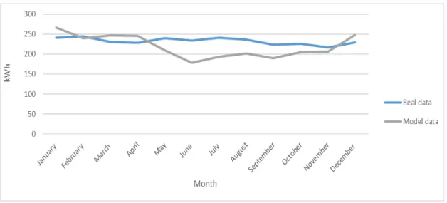
For the first house, the measured data comprehends months from May to September of the year 2015. This means that the runs of the model focus in these months exclusively. Each run has the same allocation of appliances, what differs is the month (see Annex 1). The results obtained are the followings:
Table 4.1. Data obtained from the simulation of the model and real data of the first house in study.
Month Real Data (kWh) Model Data (kWh) Error % Absolute error %
37 In Figure 4.1, it can be appreciated the data plotted side by side. By inspection, it can be seen that the match is not direct but the overall trend of electricity consumption is perceived.
Figure 4.1. First house measured and model data annual profile.
Using the software MiniTab, a Mann-Whitney U test was run on to determine if there were differences in engagement score between the data median engagement score for real data (363) and synthetic data (388,15). The results express that the data is not statistically significantly different p = 0,3785, (p>0,05) with 95,47% archived confidence.
38
Figure 4.2. Different simulated daily profiles of a weekday of January.
For the second house, the measured data comprehends months from June to November of the year 2015. The results obtained are the followings:
Table 4.2. Data obtained from the simulation of the model and real data of the second house in study.
Month Real Data (kWh) Model Data (kWh) Error % Absolute error
%
June 676 685,3 -1,3 1,3
July 836 756,7 9,5 9,5
August 875 810,3 7,4 7,4
September 976 1068,2 -9,4 9,4
October 921 902,6 2,0 2,0
November 858 807,6 5,9 5,9
39 Also, it has to be taken into account that there are more inhabitants in the second house; therefore, the consumption has more variables that might affect the unsystematic results in the model. The original statistic data of house occupancy comprehends many thousands of 1-day diaries recorded at a 10-minute resolution. This represented a barrier to certainly prove the similarities with Costa Rican behaviour, since there are not studies of this kind available. However, the overall trend involves similar patterns, which are represented in the obtained results.
Figure 4.3. Second house measured and model data annual profile.
For the data sets, Mann-Whitney U test was also performed to determine if there were differences in engagement score between the data median engagement score for real data (866,5) and synthetic data (808,9). The results express that the data is not statistically significantly different p = 0,5752, (p>0,05) with 95,47% archived confidence.
Overall, variations in different load categories are attributed only to the differences in the total daily energy demand, as no specific behavioural differences such as seasonal dependent occupancy profiles or seasonal categories share are taken into account in the model.
40 day corresponds to the assign value for the simulation of the whole month. This implies the same lighting profiles for each day throughout the month, which has direct effects in the demand of electricity.
As well, the model seeks to emulate the variability of occupancy but it may be over-representing it with lower energy use, due to various factors that are not included in the model such as multitasking. Also another important factor not included but affects directly the energy demand is the energy aware. This last element depends strictly on the costumes of the occupants and their conscious of their energy use.
4.2. VALIDATION OF THE MODEL: PV ON SITE POWER GENERATION
The following tables (Table 4.4, 4.5 and 4.6) are meant to compare the simulated data with the annual measured data of three different PV systems. According to Molar, (2015) the common system losses comprehend a total of 7%: which 1% corresponds to shading, 2% to soiling losses due to dirt and other foreign matter on the surface of the PV module, and 2% to wiring. Besides the inverter efficiency is 98% so an additional loss of 2% is considered. This parameter can be changed in the computation of the model.
The input configuration in the model is shown in Table 4.3, all the variables in this table were maintained constant for the evaluated PV systems. However, the total PV array area was changed due to different quantity of micro inverters in each system. To estimate the total PV area of each system, it was assumed a value of 1.76 m2 for each micro inverter, an azimuth angle of 0°-10° (this to indicate the software to calculate the results with a south
orientation) and a standard tilt angle. Therefore, the first, second and third PV systems, that were evaluated, had a total array area of 10.5, 29.5 and 49 m2 respectively.
41
Table 4.3. Values used in the simulation of the PV power generation on-site model.
User input/manufacturer data Value
The first PV system of 6 micro inverters south orientated is located in Heredia, Costa Rica. The measured data from January and February correspond to the year 2016, meanwhile the rest of the months are from 2015. Depicted in Table 4.4, the months of June and July have the biggest percentage of error; meanwhile the month of March has the smallest one. These differences can also be appreciated in Figure 4.4.
Table 4.4. Data obtained and simulated of a system with 6 micro inverters. Month
September 223,488 190,449 14,783 14,783
October 226,169 204,472 9,593 9,593
November 216,278 206,084 4,713 4,713
December 229,074 248,141 -8,323 8,323
42
Figure 4.4. Annual energy produced by a PV installation of 6 micro inverters.
As well, the Mann-Whitney U test was run on to determine if there were differences in engagement score between the data. Median engagement scored for real data (232,129) and synthetic data (388,15). The two groups did not differ significantly, p = 0,3708 (p>0,05) with 95,36% archived confidence.
One of the problems to be emphasised is the wide fluctuation in the irradiance conditions in the Central Valley, even in just small distances of 20 kilometres. This is caused by the influence of local clouds and microclimates in the valley (Weigl, 2014). Thus, this represents a barrier in the modelling, due to the fact that high-resolution irradiance profiles are obtained from the meteorological station of Fabio Baudrit, which means that the locations are not the same. Even though the proximity of this station is close to the PV systems in study, the distance represents a barrier to the accuracy of the results modelled.
Nonetheless, because significant spatial differences in irradiance exist, it is crucial to determine the unique solar irradiance profile for each PV site to analyse the impact of high PV penetration. Hence, to exemplify how the model can simulate appropriately the PV penetration, two different sky conditions were analysed using minute data of the month of February; measured and synthetic (see Figure 4.5 and 4.6).
43
Figure 4.5. On-site electricity profile generated with clear sky conditions.
Figure 4.6. On-site electricity profile generated with cloudy sky conditions.
44 scattering unshaded areas do not necessarily receive 100% of clear sky irradiance. On the other hand, shaded areas can receive considerably more than zero irradiance due to considerable diffuse horizontal irradiance even on cloudy days (Nguyen et al., 2016).
The second PV system is located in Puntarenas, Costa Rica. The PV system array consists of 9 micro inverters south orientated and 8 east orientated for a total of 17 micro inverters. The results are shown in Table 4.5.
Table 4.5. Data obtained and simulated of a system with 17 micro inverters.
Month Real Data
45
Figure 4.7. Annual energy produced by PV installation of 17 micro inverters.
The Mann-Whitney U test was run on to determine if there were differences in engagement score between the data. Median engagement score for real data (595,572) and synthetic data (575,547). It was proven that they are not statistically significantly different, p = 0,7075, (p>0,05) with 95,36% archived confidence.
Since the system has almost half of the micro inverters orientated to the east, in order to analyse the effect in Figure 4.8, it is shown a clear sky day profile of the month of February. Both measured data and simulated data belong to this month.
46
Figure 4.8. On-site electricity profile generated with clear sky conditions
The last PV system evaluated is located in San José, Costa Rica. The PV system array consists of 22 micro inverters south orientated and 6 west orientated for a total of 28 micro inverters. The results are shown in Table 4.6. From January to April the data is from 2016, the rest of the monthly data corresponds to the year 2015.
Table 4.6. Data obtained and simulated of a system with 28 micro inverters.
Month Real Data
(kWh)
Model Data (kWh) Error % Absolute error %
January 1069,113 1212,976 -13,456 13,456
February 1054,507 1091,070 -3,467 3,467
March 1122,753 1125,007 -0,201 0,201
April 1019,589 1119,206 -9,770 9,770
May 828,573 956,560 -15,447 15,447
June 729,022 812,243 -11,416 11,416
July 741,472 882,154 -18,973 18,973
August 842,333 919,370 -9,146 9,146
September 692,273 868,092 -25,397 25,397
October 825,076 932,012 -12,961 12,961
November 796,485 939,359 -17,938 17,938
December 949,001 1131,063 -19,184 19,184
47 In this case the month with the biggest absolute error percentage corresponds to September. March has the smallest value. In Figure 4.9, it can be appreciated the similarities in the patterns of the data throughout the year, and a noticeable gap of approximately 100 kWh from April to November.
Figure 4.9. Annual energy produced by PV installation of 28 micro inverters.
Likewise, for the data sets, a Mann-Whitney U test was run on to determine if there were differences in engagement score between the data. Median engagement score for real data (835,453) and synthetic data (947,960). The results expressed that the groups are not statistically significantly different, p = 0,0606 with 95,36% archived confidence.
48 Attention should also be drawn to the fact that the output of a large PV system will not be interrupted immediately when a small cloud begins to pass over and gradually shades the array. Instead, there will be an averaging effect and the cloud-caused variation of the PV power output will be smooth rather than sharp.
On the other hand, for smaller areas, the time frame between maximum generation (clear sky) and low generation (which means that the array completely shaded by clouds) tends to be much shorter. The reason is that it takes less time for a cloud shadow to cover the entire array area. As well, the incident solar radiation from shadows caused by objects near the PV array plays an important role.
4.3. MATCHING INDEXES
In order to evaluate the impact of the time resolution on the matching of PV production and electricity demand data of the first house previously evaluated in section 4.1 and a south oriented PV system of approximately 11 m2 was analysed. Three different sky conditions were evaluated: clear sky, partially cloudy sky and cloudy sky; to perceive the different scenarios on variable weather conditions fitting to the seasons of the year in Costa Rica. Daily profiles were taken from the month of March (see Figures 4.10, 4.11 and 4.12), which correspond to dry season and from the month of August (see Figures 4.13, 4.14 and 4.15), which correspond to the wet season.
49
Figure 4.10. Dry season day with clear sky on-site electricity generation profile.
50
Figure 4.12. Dry season day with cloudy sky on-site electricity generation profile.
51
Figure 4.14. Wet season day with cloudy sky on-site generation profile.
52 It can be observed in Figures 4.10 and 4.13 the smoothness of the profiles. The slight averaging effect in clear sky conditions in comparison with the other sky conditions assured that the profiles are less sensitive to this.
On the other hand, a noticeable difference between the resolution profiles is shown in partially cloudy sky conditions (see Figures 4.11 and 4.14).
The averaging effect expressed by the hour resolution clearly differs from the minute resolution because the constant output power fluctuates provoked by the rapidly oscillation of the solar radiation intensity in a time scale ranging from several minutes to a few seconds (Cao & Sirén, 2014). Therefore, the impact of coarser resolution is bigger when sky conditions are partially cloudy or cloudy as well (see Figures 4.12 and 4.15).
It can be appreciated that the season does not have a major impact in the PV power production. Consequently, the solar production fluctuates only slightly through the year. Therefore, data exclusively from the month of March was used to effectuate further analysis. The error in the matching was calculated to consider it in the matching results triggered by different resolutions. The results are shown in Table 4.7.
Table 4.7. eOEM and eOEF error results in different sky conditions of the month of March.
Clear sky Partially cloudy sky Cloudy sky
!!"# !!"# !!"# !!"# !!"# !!"#
10,32% 10,20% 39,18% 39,02% 37,86% 37,70%
The mean error, in all the scenarios, shows the overestimation of the amount of electricity demand that can be covered by the PVs and the consumption of energy produced. The stronger impact occurs for partially cloudy sky conditions where both !!"# and !!"# are bigger.