New insights into the use of stable water isotopes at the northern Antarctic Peninsula as a tool for regional climate studies

https://doi.org/10.5194/tc-12-1069-2018

© Author(s) 2018. This work is distributed under the Creative Commons Attribution 3.0 License.

New insights into the use of stable water isotopes at the northern

Antarctic Peninsula as a tool for regional climate studies

Francisco Fernandoy1, Dieter Tetzner2, Hanno Meyer3, Guisella Gacitúa4, Kirstin Hoffmann3, Ulrike Falk5, Fabrice Lambert6, and Shelley MacDonell7

1_{Facultad de Ingenieria, Universidad Andres Bello, Viña del Mar, 2531015, Chile}

2_{Center for Climate and Resilience Research, Universidad de Chile, Santiago, 8370361, Chile} 3_{Alfred Wegener Institute Helmholtz Centre for Polar and Marine Research, Research Unit Potsdam,}

Telegrafenberg A43, 14473 Potsdam, Germany

4_{Programa GAIA-Antártica, Universidad de Magallanes, Punta Arenas, 6210427, Chile} 5_{Climate Lab, Geography Department, University Bremen, 28334 Bremen, Germany}

6_{Department of Physical Geography, Pontificia Universidad Católica de Chile, Santiago, Chile} 7_{Centro de Estudios Avanzados en Zonas Áridas (CEAZA), La Serena, Chile}

Correspondence:Francisco Fernandoy ([email protected]) Received: 30 December 2016 – Discussion started: 24 January 2017

Revised: 3 February 2018 – Accepted: 15 February 2018 – Published: 26 March 2018

Abstract.Due to recent atmospheric and oceanic warming, the Antarctic Peninsula is one of the most challenging re-gions of Antarctica to understand in terms of both local- and regional-scale climate signals. Steep topography and a lack of long-term and in situ meteorological observations com-plicate the extrapolation of existing climate models to the sub-regional scale. Therefore, new techniques must be de-veloped to better understand processes operating in the re-gion. Isotope signals are traditionally related mainly to atmo-spheric conditions, but a detailed analysis of individual com-ponents can give new insight into oceanic and atmospheric processes. This paper aims to use new isotopic records col-lected from snow and firn cores in conjunction with existing meteorological and oceanic datasets to determine changes at the climatic scale in the northern extent of the Antarc-tic Peninsula. In parAntarc-ticular, a discernible effect of sea ice cover on local temperatures and the expression of climatic modes, especially the Southern Annular Mode (SAM), is demonstrated. In years with a large sea ice extension in winter (negative SAM anomaly), an inversion layer in the lower troposphere develops at the coastal zone. Therefore, an isotope–temperature relationship (δ–T) valid for all peri-ods cannot be obtained, and instead theδ–T depends on the seasonal variability of oceanic conditions. Comparatively, transitional seasons (autumn and spring) have a consistent

isotope–temperature gradient of+0.69 ‰◦C−1. As shown by firn core analysis, the near-surface temperature in the northern-most portion of the Antarctic Peninsula shows a de-creasing trend (−0.33◦C year−1) between 2008 and 2014. In addition, the deuterium excess (dexcess) is demonstrated

to be a reliable indicator of seasonal oceanic conditions, and therefore suitable to improve a firn age model based on seasonaldexcessvariability. The annual accumulation rate

in this region is highly variable, ranging between 1060 and 2470 kg m−2year−1from 2008 to 2014. The combination of isotopic and meteorological data in areas where data exist is key to reconstruct climatic conditions with a high temporal resolution in polar regions where no direct observations ex-ist.

1 Introduction

rapid warming of both atmosphere and ocean has caused ice shelf instability in West Antarctica, especially in some re-gions of the AP (Pritchard et al., 2012). Instability leading to ice shelf collapse has triggered accelerated ice-mass flow and discharge from land-based glaciers into the ocean, as the ice shelves’ buttressing function is lost. Accelerated rates of ice mass loss (Pritchard and Vaughan, 2007; Rignot et al., 2005; Pritchard et al., 2012) in combination with increased surface snow melt, has contributed to a negative surface mass bal-ance especially in the northern part of the AP region (Harig and Simons, 2015; Seehaus et al., 2015; Dutrieux et al., 2014; Shepherd et al., 2012).

The glaciers of the AP have lost ice mass at a rate of ap-proximately 27 (±2) Gt year−1between 2002 and 2014. This mass loss combined with the mass loss over the West Antarc-tic Ice Sheet (121 (±8) Gt year−1), surpassed the mean pos-itive mass balance of +62 (±4) Gt year−1 _{observed in East}

Antarctica, of which most of the positive balance relates to the Dronning Maud Land region whereas the mass balance of the rest of the EAIS is at equilibrium (Harig and Simons, 2015). This demonstrates how vulnerable the coastal region of West Antarctica is to increased air and sea surface temper-atures (Bromwich et al., 2013; Meredith and King, 2005).

Surface snow and ice melt on the AP represents up to 20 % of the total surface melt area (extent) and 66 % of the melt volume from Antarctica for at least the last three decades (Trusel et al., 2012; Kuipers Munneke et al., 2012). Regional positive temperatures detected by remote-sensing techniques and ice-core data reveal that melt events have been temporally more widespread since the mid-20th cen-tury (Abram et al., 2013; Trusel et al., 2015), with some se-vere melt events during the first decade of the 21st century (Trusel et al., 2012). Increased surface melt and glacier calv-ing are likely to have freshened upper ocean layers and there-fore impacted biological activity in the coastal zone (Mered-ith et al., 2016; Dierssen et al., 2002). The most signifi-cant warming trend detected at the AP coast occurred dur-ing the winter season, especially on the western side of the peninsula, where a positive trend of>0.5◦C decade−1for the period 1960–2000 has been reported at several stations (Turner et al., 2005; Carrasco, 2013). For example, winter warming is especially evident in daily minimum and monthly mean temperature increases, as described by Falk and Sala (2015) for the meteorological record of the Bellingshausen Station on King George Island (KGI) at the northern AP during the last 40 years. In KGI the daily mean tempera-ture during winter increased at about 0.4◦_{C decade}−1_{, with}

a marked warming during August (austral winter) at a rate of+1.37 (±0.3)◦C decade−1. Positive temperatures even in winter are more commonly observed, leading to more fre-quent and extensive surface melting year-round especially for the northern AP, which is dominated by maritime climate conditions (Falk and Sala, 2015).

The mechanisms causing increasing atmosphere and ocean temperatures are still not completely understood but

can be linked to perturbations of regular (pre-industrial pe-riod) atmospheric circulation patterns (Pritchard et al., 2012; Dutrieux et al., 2014). Most heat advection to the south-ern ocean and atmosphere has been related to the poleward movement of the Southern Annular Mode (SAM) and to some extent to the El Niño Southern Oscillation (ENSO) (Gille, 2008; Dutrieux et al., 2014; Fyfe et al., 2007). Dur-ing the last decades, SAM has been shiftDur-ing into a positive phase, implying lower than normal (atmospheric) pressures at coastal Antarctic regions (latitude 65◦S) and higher (at-mospheric) pressures over the mid-latitudes (latitude 40◦S) (Marshall, 2003). As a result of lower pressures around Antarctica, the circumpolar westerly winds increase in in-tensity (Marshall et al., 2006). As a consequence, air masses transported by intensified westerlies overcome the topogra-phy of the AP more frequently, especially in summer, bring-ing warmer air to the east side of the AP (van Lipzig et al., 2008; Orr et al., 2008). The correlation between the SAM and surface air temperature is generally positive for the AP, explaining a large part (∼50 %) of near-surface temperature increase for the last half century (Marshall et al., 2006; Mar-shall, 2007; Carrasco, 2013; Thompson and Solomon, 2002). An enhanced circulation enables more humidity to be trans-ported to and trapped at the west coast of the AP due to the orographic barrier of the central mountain chain. This has re-sulted in the consistent increase of accumulation across the entire AP during the 20th century, thereby doubling the ac-cumulation rate from the 19th century in the southern AP re-gion (Thomas et al., 2008; Goodwin et al., 2015; Dalla Rosa, 2013).

The increase of greenhouse gas concentrations and the stratospheric depletion of the ozone layer, both linked to anthropogenic activity, are thought to be the main forcing factors of the climate shift that has affected the ocean– atmosphere–cryosphere system for at least the last half cen-tury (Fyfe and Saenko, 2005; Sigmond et al., 2011; Fyfe et al., 2007).

The lack of long-term meteorological records limits accu-rate determination of the onset and regional extent of this cli-mate shift. Therefore, clicli-mate models are needed to extend the scarce climate data both spatially and temporally. One major challenge is to correctly integrate the steep and rough topography of the AP into climate models. To facilitate this, more detailed information of surface temperatures, melting events, accumulation rates, humidity sources and transport pathways are urgently needed. As direct measurements of these parameters are often not available, the reconstruction of the environmental variability, basically relies on proxy data such as the stable water isotope composition of precipitation, firn and ice (e.g., Thomas and Bracegirdle, 2009; Thomas et al., 2009; Abram et al., 2013).

and melt events on the AP and their relationship with atmo-spheric and oceanic conditions i.e., sea surface temperature, humidity and sea ice extent. We investigate the effects of the orographic barrier of the AP on air mass and moisture trans-port, with increasing precipitation rates from the coast to the mountain range on the Peninsula divide at ca. 1100 m a.s.l. (Fernandoy et al., 2012a), where the ice thickness reaches ca. 350 m at maximum (Cárdenas et al., 2014).

2 Glaciological setting and previous work

Since 2008 we have undertaken several field campaigns to the northernmost region of the AP, where we have retrieved a number of firn cores of up to 20 m depth. The present inves-tigation is the first of its kind for this sector of the AP. Other studies have been carried out further south at Detroit Plateau (Dalla Rosa, 2013) and Bruce Plateau (Goodwin et al., 2015), approximately 100 and 400 km southwest of the northern AP. Nonetheless, not much is known about the glaciolog-ical conditions at the northern tip of the AP and very few ice cores have been retrieved from this area despite the high number of scientific stations in the region (Aristarain et al., 2004; Simões et al., 2004; Goodwin et al., 2015; Fernandoy et al., 2012a; Dalla Rosa, 2013). The AP and subantarctic islands are principally characterized by mountain glaciers or small ice caps, which flow into the Bellingshausen and Weddell Sea to the west and east, respectively (Turner et al., 2009). Rückamp et al. (2010) noted that the ice cap cover-ing Kcover-ing George Island, South Shetlands (62.6◦S, 60.9◦W) is characterized by polythermal conditions and temperate ice at the surface (>−0.5◦C), and is therefore sensitive to small changes in climatic conditions. Further south, Zagorodnov et al. (2012) showed that temperatures from boreholes reach a minimum at 173 m depth (−15.8◦C) at Bruce Plateau (66.1◦S, 64.1◦W, 1975.5 m a.s.l.). Similar glaciological con-ditions were reported on the east side of the AP at James Ross Island (64.2◦_{S, 57.8}◦_{W, 1640 m a.s.l.) (Aristarain et al.,}

2004). Accumulation rates at the northern AP are directly related to the westerly atmospheric circulation and mar-itime conditions, with values close to 2000 kg m−2year−1on the west side (Goodwin et al., 2015; Potocki et al., 2016) and lower values (∼400 kg m−2year−1) on the eastern side (Aristarain et al., 2004). Ice thickness from all coring-sites reported is<500 m to the bedrock.

3 Methodology

3.1 Field work and sample processing

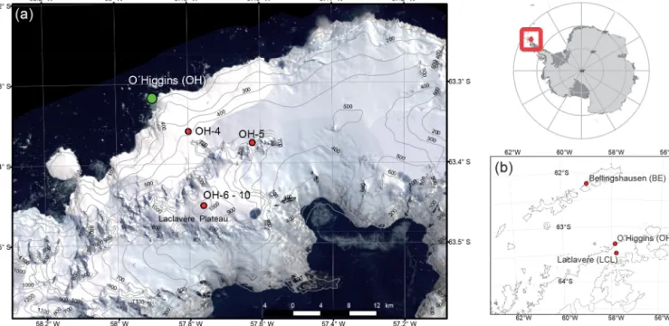
During five austral summer campaigns (2008–2010, 2014, 2015), an altitudinal profile was completed from sea level near O’Higgins Station (OH) to 1130 m a.s.l.at the Laclavère Plateau (LCL) (Fig. 1). In total, five firn cores are included in this paper: OH-4, OH-5, OH-6, OH-9, OH-10 (Fig. 1);

coordinates and further details of the firn cores are given in Table 1. Two hundred and eight daily precipitation samples were gathered at the meteorological observation site of the O’Higgins Station (57.90◦W, 63.32◦S, 13 m a.s.l.) during 2008–2009 (Fernandoy et al., 2012a) and 2014 (Table 2). The overwintering crew at O’Higgins Station collected daily pre-cipitation samples from pluviometers installed at the mete-orological observation site. Each daily sample comprised of a filling a narrow neck HDPE type bottle with a 30 mL com-posite sample of the precipitation (both liquid and solid) that fell in the previous 24 h. The bottles were tightly closed and stored frozen year-long to ensure correct storage and to facil-itate the subsequent transport to the laboratory at the end of each year. From these samples, approximately 6 % (13 sam-ples) were discarded from the analysis due to improper stor-age causing leakstor-age from the bottles. Improper storstor-age was assessed using a statistical outlier test (modified Thompson tau technique) that indicated unusual values of stable water isotope analyses.

Figure 1.Study area and location of the firn cores presented in this work.(a)Detail of the study zone: the green point shows the Chilean Station O’Higgins (OH) on the west coast of the Antarctic Peninsula. Firn cores retrieved between 2008 and 2015 are shown by red dots. (b) Location of O’Higgins and Bellingshausen Station and Laclavère Plateau, which are mentioned throughout the text. Satellite image (Landsat ETM+) and digital elevation model (RADARSAT) available from the Landsat Image Mosaic of Antarctica (LIMA) (http://lima. usgs.gov/).

Table 1.Statistical summary of the geographical location and water stable isotope composition of all firn cores examined in this work. OH-4 and OH-5 correspond to cores retrieved on the west side of the AP, whereas OH-6, OH-9 and OH-10 were retrieved at LCL on the east-west divide. All cores were analyzed in a 5 cm resolution.

Core OH-4 OH-5 OH-6 OH-9 OH-10

Coordinates 57.80◦W, 63.36◦S 57.62◦W, 63.38◦S 57.76◦W, 63.45◦S 57.76◦W, 63.45◦S 57.76◦W, 63.45◦S

Altitude (m a.s.l.) 350 620 1130 1130 1130

Depth (m) 15.8 10.6 11.0 11.7 10.2

Drilling date Jan 2009 Jan 2009 Jan 2010 Jan 2014 Jan 2015

δ18O (‰)

Mean −10.4 −10.2 −12.0 −12.8 −12.9

SD 1.2 1.5 2.5 2.5 2.6

Min −14.1 −14.2 −19.8 −23.3 −21.9

Max −7.0 −7.2 −6.5 −8.1 −7.3

δD (‰)

Mean −78.9 −78.1 −91.4 −97.5 −98.8

SD 9.7 12.0 19.4 21.0 20.5

Min −108.2 −111.2 −154.9 −183.8 −166.8

Max −54.0 −52.1 −53.2 −59.6 −55.8

dexcess(‰)

Mean 4.0 3.9 4.4 5.1 4.7

SD 1.5 1.7 2.8 1.9 2.7

Min 0.5 −0.6 −2.6 0.0 −6.5

Max 8.6 8.2 15.0 11.0 11.3

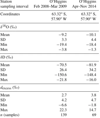
Table 2.Statistics of the stable water isotope composition of precip-itation samples collected at OH Station on the AP 2008–2009 and 2014.

Station O’Higgins O’Higgins

sampling interval Feb 2008–Mar 2009 Apr–Nov 2014

Coordinates 63.32◦S, 63.32◦S,

57.90◦W 57.90◦W oxygen and hydrogen isotopes, respectively.

3.2 Database and time series analysis

Stable water isotope data were compared to major mete-orological parameters from the region (Fig. 2). For this purpose, the following data sets were incorporated into our analysis: daily and monthly near-surface air tempera-ture (Tair), precipitation (Pp) and sea-level pressure (SLP)

measurements recorded at the Bellingshausen Station (BE) (58.96◦W, 62.19◦S, 15.8 m a.s.l.) and the O’Higgins Sta-tion (OH). These datasets were downloaded from the Global Summary of the Day (GSOD) from the National Climatic Data Center (NCDC, available at: www.ncdc.noaa.gov) and the SCAR Reference Antarctic Data for Environmental Re-search (READER, available at: https://legacy.bas.ac.uk/met/ READER/) (Turner et al., 2004).

The temperature record from OH contains several large data gaps, and so the available data from 1968 to 2015 were compared with those measured at BE to evaluate the possibil-ity of lapsing data from BE to the site due to the data continu-ity available (uninterrupted record since 1968). The BE and OH data are highly correlated (R=0.97,p <0.01), and so a correction of−1.4◦C was applied to the BE data based on linear regression analysis. Other nearby stations such as Es-peranza (63.40◦S, 57.00◦W), were not considered because

95

2008 2009 2010 2011 2012 2013 2014 2015

(a)

(b)

(c)

(d)

(e)

Figure 2. Monthly meteorological data sets used in this study

(a) sea surface temperature (SST), (b) air temperature (Temp), (c) sea level pressure (SLP) and (d) precipitation amount (Pre-cip) from Bellingshausen Station (BE) on King George Island and (e) relative humidity (rh) from the Southern Ocean surrounding the northern Antarctic Peninsula (AP). Data shown in the figure is available from the READER dataset (https://legacy.bas.ac.uk/met/ READER/) (Turner et al., 2004).

of a slightly lower correlation (R=0.96,p <0.01) and the possibility of a higher continental influence on the tempera-ture record.

Sea surface temperature (SST) time series were extracted from the Hadley Centre observation datasets (HadSST3, available at: http://www.metoffice.gov.uk/hadobs/hadsst3/). The HadSST3 provides SST monthly means on a global 5◦ by 5◦grid from 1850 to present (Kennedy et al., 2011a, b). Mean monthly SSTs were extracted from a quadrant limited by 60–65◦S and 65–55◦W. Missing data or outliers were interpolated from measurements taken in neighboring quad-rants.

were obtained from backward trajectories arriving under iso-baric conditions (850 hPa) at the OH station. SST and rh datasets were resampled to a regional scale defined by high-density trajectory paths (Bellingshausen and Weddell Seas). The resampled fields were defined by the spatial coverage of 1-day backward trajectories. The limits of the resulting quad-rant extends from 98 to 34◦W longitude and from 47 to 76◦S latitude. The covered area is representative of the study site because it includes the region affected by westerly winds and sea ice front during winter time, both factors that exert a high influence on approaching air parcels. A field horizontal mean of resampled rh values between sea level and 150 m a.s.l.was computed for this area to construct the rh time series used throughout this study.

Altitudinal temperature profiles were obtained from ra-diosonde measurements carried out at BE between 1979 and 1996 (SCAR Reference Antarctic Data for Environmental Research). Lapse rates were calculated from the tempera-ture difference between sea level and the 850 hPa level. SAM index time series were obtained from the British Antarctic Survey (BAS, available at: http://legacy.bas.ac.uk/met/gjma/ sam.html) (Marshall, 2003). Mean monthly sea ice extent around the AP (between 1979 and 2014) was obtained from the Sea Ice Index from the National Sea & Ice Data Cen-ter (NSIDC, available at http://nsidc.org). The measurements of sea ice extension incorporated in this study considered as a starting point the coastal location of OH, and the sea ice front in the direction towards KGI as an end point.

3.3 Stable isotope time series analysis

Firn and ice core ages are often dated by analyzing the sea-sonality of stable water isotope values. In the firn cores an-alyzed in this study, there was a significant difference in the standard deviation (SD>1.0) of high resolution (5 cm) oxy-gen isotopes values between firn cores from lower altitudes (OH-4,δ18O SD=1.2) vs. cores from higher altitudes (OH-10,δ18O SD=2.6) (Table 1). However, within each individ-ual core, the raw datasets obtained from stable water isotope analysis (Sect. 3.1) produced low oscillation variance in the isotope-depth profile. Whilst the measured isotope signals were noisy, the values do not fluctuate far from each core’s mean. This low variance, added to the fact that the patterns described in the isotope-depth profiles do not correspond to seasonal cycles, means that dating each core using traditional annual layer counting is complicated. Difficulties from using conventional dating methodology for these firn cores led us to search for other ways to define the time scale of our sig-nals.

We first analysed thedexcessdata, becausedexcessis related

to seasonal oceanic conditions, and therefore displays an an-nual signal in this region (Fernandoy et al., 2012a). Whilst the stable water isotope results did not display a regular pat-tern, the dexcess is characterized by a noisy, low frequency

oscillation. We use this low-frequency periodic signal to date the core (see below).

We calculated theoreticaldexcess values at our site using

the relationship between rh and SST computed by Uemura et al. (2008):dexcess meteo= −0.42×rh+0.45×SST+37.9.

The suitability of using this relationship for the AP region was assessed by comparing thedexcess measurements of the

daily precipitation samples taken at the OH station with the corresponding theoretical values. For each day that a precipi-tation sample was collected at OH, 3-day air parcel backward trajectories were calculated using the HYSPLIT model. We identified frequent air parcel paths and calculated monthly mean values of rh and SST from re-analysis data (GDAS) along these paths. We found a very good agreement between the measured and our theoreticaldexcessvalues, with a

corre-lation ofR=0.86 (p <0.01). This high correlation allows us to directly compare a synthetic dexcess meteo time series

and the observationaldexcess record obtained from each firn

core. For the method to be successful, the resultant depth-age model should maximize the common variability between the two time series.

Thedexcesssignal obtained from stable isotope analysis of

firn cores is measured with respect to depth (i.e., in the space domain). To extract the low frequency seasonal signal, we first computed the fast Fourier transform (FFT) of thedexcess

data, which identifies all the frequencies in the record. For each of the signals, we defined a cut-off frequency for each core using the peak with the second lowest frequency iden-tified in the amplitude spectrum (Table 4). We then recon-structed the low-frequencydexcess signal by calculating the

inverse fast Fourier Transform (IFFT) from the lowest two identified frequency peaks

We applied the same procedure to the monthly means of the syntheticdexcess meteo time series, thus obtaining two

low-frequency signals that should show the same seasonal variability due to their dependency on the same variables (i.e., environmental condition of the moisture source re-gion). We then chose a linear depth-age model that visually matched the variability in the low-frequency observational dexcess data with the variability in the low-frequency

syn-theticdexcess meteodata. A single linear stretching factor was

calculated using that relationship and applied to the complete firn cores datasets. We used the same depth-age model to put the firn coreδ18O records on a time axis for further analysis using monthly means.

4 Results

4.1 Precipitation samples

lo-2015 2015

2014 2014

2013 2013

2012 2012

2011 2011

2010 2010

2009 2009

2008 2008

8 4

0 -20 -16 -12 -8

dexcess ‰ VSMOW δ18O ‰ VSMOW

Year (C.E.)

OH-10

OH-9

OH-6

5 cm resolution δ18O and dexcess Monthly mean

dexcess d_{excess meteo} δ18O

(b) (a)

Figure 3. Time series for firn cores OH-6 (light blue line right), OH-9 (green light right) and OH-10 (purple line right) derived for

δ18O (bold black line middle left panel) anddexcess (red line left panel) records using a theoreticaldexcess(dexcess meteo) value (blue line left panel). The dexcess meteo is calculated from sea surface temperature (SST) and relative humidity (rh) according to Uemura et al. (2008). All three cores are located at the same location within the GPS navigator horizontal error (<10 m).

cal meteoric water line (LMWL):δD=7.83×δ18O−0.12. Backward trajectory analysis of precipitation events reveals high-frequency transport across the Bellingshausen Sea dur-ing the 24 h before the air parcels reach the AP (Fig. 5). 4.1.1 Isotope–temperature relationship

The relationship between the stable water isotope composi-tion of daily precipitacomposi-tion events and daily near-surface tem-perature (Tdaily) at OH was assessed using linear regression

analysis of a sample set of measurements. The sample popu-lation consisted of the months with the largest number of pre-cipitation samples (namely December 2008, March 2008 and 2009, June 2008 and October 2014). Only selected months were analyzed to ensure the most complete set of data within a relatively short timeframe to improve the derivation of the calculated relationship. Outliers, given by anomalous dexcess values (see Sect. 3.1,dexcess<−9 ‰), were filtered

out in order to avoid disturbances in the model, as the qual-ity of these samples was likely compromised during storage and transport. It should be noted that this relationship will be compared to firn core time series in Sect. 4.2.2, in order to reconstruct the air surface temperature at Laclavère Plateau.

Additionally, to investigate the relationship at a monthly scale, a correlation was performed for monthly means cal-culated from daily events (δ18Omonthly; Tmonthly) over the

24 month long precipitation dataset (February 2008 to March 2009, and April–November 2014) (Table 3). Con-siderable differences were identified between the daily and monthlyδ18O–T relationships (Table 3; Fig. 4a), which indi-cated that the isotope–temperature relationship is seasonally-dependent. The seasonality of this relationship was deter-mined using the linear regression slope (s) of the dailyδ18O– T relationship (see Table 3 for statistical details). The sea-sonal linear regression between δ18O and Tdaily based on

208 precipitation events revealed correlation coefficients (R) higher than 0.6 and a statistical significance (p) lower than 0.03. To facilitate the evaluation of seasonal signals, the daily datasets were categorized by season, such that: austral summer (December–January–February, DJF) was character-ized using December 2008 data; austral autumn (March– April–May, MAM) was characterized using March 2008 and 2009 data; austral winter (June–July–August, JJA) by June 2008 data; and austral spring (September–October– November, SON) by October 2014 data. If MAM and SON are combined together, considering they are both shoulder seasons, theδ18O–T relationship is defined by the linear re-gression:δ18O=0.79×Tdaily−7.76 (R=0.74,p <0.01).

For austral summer, the δ18O–T relationship can be ex-pressed as:δ18O=1.17×Tdaily−8.19 (R=0.81,p=0.01);

and austral winter as:δ18O=0.35×Tdaily−8.66 (R=0.63,

p=0.01).

4.1.2 Deuterium excess–temperature relationship Deuterium excess (dexcess) was calculated for each

precipi-tation sample from stable water isotope data obtained at OH (see Table 2 for descriptive statistics). To evaluate the prox-imity to the original evaporation source for each precipita-tion sample, we examined both the isotope–temperature re-lationship as well as the near surface temperature anddexcess

relationship using linear regression analysis. As for the eval-uation of the isotope–temperature relationship (Sect. 4.1.1), daily dexcess values for December 2008, March 2008 and

2009, June 2008 and October 2014 were compared with daily mean temperatures, however, correlation coefficients were not significant (Table 3). For the 2008-09 datasets, the dexcess–T correlation for monthly averages (calculated from

daily events as outlined in Sect. 4.1.1) was significant (Ta-ble 3; Fig. 4b), and the associated linear regression was cal-culated to be:dexcess= −0.60×Tmonthly+2.12 (R= −0.77,

p <0.01). For the 2014 dataset the correlation is not signifi-cant (R=0.33,p >0.05).

4.1.3 Moisture source of precipitation

Jan Feb Mar Apr May Jun Jul Aug Sep Oct Nov

Month

0 2 4 6 8 10 12 14 16 18

Sa

m

pl

e

nu

m

be

r (

n)

2008 2009 2014

(c) -15

-10 -5

δ

18 O

VSMOW

‰

May/08 Sep/08 Jan/09

Month/year (CE)

May/14 Sep/14 10

5 0 -5

dexcess

‰

-8 -6 -4 -2 0 2 Temperature (°C)

-8 -6 -4 -2 0 2 Temperature (°C) (a)

(b)

Precipitation events δ18O‰ Monthly mean

δ18O‰ Temperature

Precipitation events

d_excess ‰

Monthly mean

d_excess ‰

Temperature

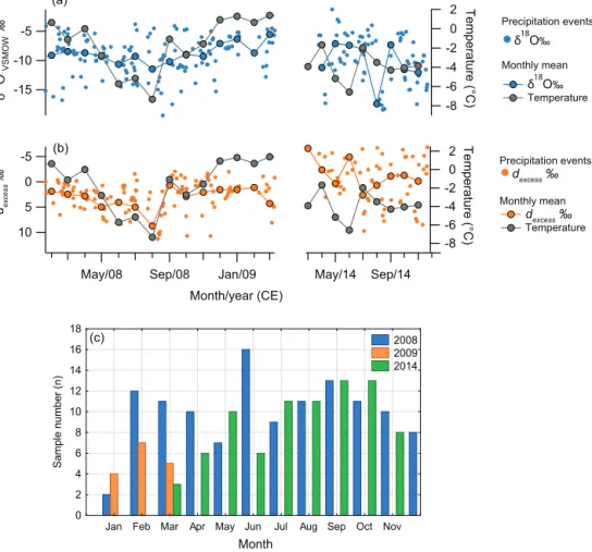
Figure 4.Stable water isotope composition of precipitation events and air temperature at O’Higgins Station.(a)shows theδ18O composition of precipitation of single daily events (small solid blue dots) and monthly means (big solid blue dots and line) and(b)deuterium excess (dexcess) of single daily events (small orange dots) and monthly means (big orange dots and line). In both(a)and(b)monthly mean air temperature is also shown (grey solid dots and line).(c)Histogram showing the monthly distribution of precipitation samples (n) collected at O’Higgins Station in 2008, 2009 and 2014.

in part the variability of the isotope–temperature relationship presented in Sects. 4.1.1 and 4.1.2. Most of the pathways originate in the Southern Pacific Ocean and the Amundsen– Bellingshausen Seas. The trajectories are primarily derived from the Bellingshausen Sea, the Bransfield Straight and the Drake Passage, Tierra del Fuego and South America’s south-ern tip. In addition, some trajectories (<15 %) originate from AP’s eastern side. Precipitation trajectories show an almost elliptically distributed pattern with a N40◦W orientation, and most follow pathways between 60 and 67◦S. The correla-tion between monthly mean values ofdexcess (from

precip-itation samples) and dexcess meteo (constructed from the

me-teorological parameters rh and SST of the high density pre-cipitation pathways) had a significant correlation coefficient ofR=0.86 (p <0.01) (Fig. 6), demonstrating that oceanic conditions control most of the precipitation variability.

4.2 Firn core samples from the AP

Table 1 shows the stable isotope results and descriptive statis-tics for firn cores retrieved at the northern AP. The co-isotopic relationship δD–δ18O for each single firn core re-trieved from LCL is related to the global meteoric water line (GMWL) and the local meteoric water line (LMWL) (Rozan-ski et al., 1993), with a mean slope ofs=7.91 and an inter-cept of 3.64 (Fig. 7). These values are very close to those of the LMWL, although with a slightly higher intercept.

4.2.1 Age model based on stable water isotopes

Stable water isotope results from each firn core allow the derivation of individual depth profiles of δD, δ18O and dexcess for each firn core. Lowest noise values and the

clearest seasonal patterns were found in dexcess profiles

(dexcess core) (Fig. 3), similar to findings published by

W W

W

W

W

W

W

Weddell Sea Bellingshausen_Sea

O’Higgins (OH)

80° W 60° W 40° W

140° W 120° W 100° W 50° S 20° E 0° 20° W 50° S

70° S Trajectory frequency

0.1 0.5 0.9

Figure 5.Frequency distribution map of the main transport paths of air masses approaching the northern Antarctic Peninsula (AP). Translucent red colours represent the lowest frequency and blue colours the higher frequency. In general, most of the air masses ar-riving at the AP are coming from the Bellingshausen Sea and the South Pacific Ocean.

5

4

3

2

1

0

-1

-2 dex

ce

ss

m

et

eo

‰

8 6 4 2 0 -2 -4

dexcess‰

dexcess meteo=0.52 dexcess +0.81

R = 0.86

Figure 6. Correlation between monthly mean deuterium excess

values (dexcess) from precipitation samples and theoretical deu-terium excess values (dexcess meteo) calculated from meteorologi-cal parameters of the moisture source region according to Uemura et al. (2008).

Table 3.Statistical correlations and linear regression significance of theδ18O anddexcess–temperature relationship for precipitation samples. The slope and standard error are related to the linear re-gression constructed from the isotope–temperature rere-gressions at daily and monthly scales.

Corr. coef. Slope Std. Error pvalue (R) (s)

Precipitationδ18Odaily−Tdaily

DJF 0.81 1.17 0.62 0.01

MAM 0.65 0.77 2.08 <0.01

JJA 0.63 0.35 1.74 0.01

SON 0.6 0.61 2.88 0.03

Precipitationδ18Omonthly−Tmontly

All data-set 0.30 0.28 2.36 >0.05

2008–2009 0.74 0.41 1.03 <0.01

2014 −0.32 −0.77 3.60 >0.05

Precipitationdexcess−Tdaily

DJF −0.37 −0.86 1.66 >0.1

MAM 0.09 0.10 2.61 >0.1

JJA −0.28 −0.29 3.61 >0.1

SON −0.42 −0.74 5.97 >0.1

Precipitationdexcess−Tmontly

All data-set 0.06 0.07 2.98 >0.05

2008–2009 −0.77 −0.60 1.43 <0.01

2014 0.33 0.65 2.35 >0.05

from precipitation samples anddexcess meteo at sea level are

significantly correlated, which suggests a nearby moisture source precipitating in this area. The significant correlation indicates that moisture source conditions of a coastal and oceanic-proximal origin will be represented and preserved in the dexcess core record and could be used as a

chrono-logical marker. Thedexcess coresignals were first filtered for

their high frequency oscillation patterns and then the rem-nant signals were compared with the high frequency filtered dexcess meteo monthly means (see Sect. 3.3). The

compari-son betweendexcess meteo anddexcess core resulted in a close

similarity between them. Main peak–valley fitting between both signals led to a monthly mean dexcess core signal

rep-resented on a defined depth-time scale (Fig. 8). The com-parison between time series of monthly meandexcess coreand

dexcess meteodata reveals correlation coefficients ofR≥0.67

(p <0.01; degree of freedom (df) >21, see Table 4) for each individual firn core analyzed and obtained from 2006 to 2015. Table 4 summarizes correlation coefficients, statistical significances and time intervals for each firn core. From the firn cores retrieved from LCL, a single time series was con-structed and then compared to thedexcess meteotime series in

-150 -100 -50 0

δ

DVS

M

O

W

‰

-25 -20 -15 -10 -5 0

δ18OVSMOW ‰

OH-6

δD=7.95 δ18O + 4.1

OH-9

δD=7.90 δ18O + 3.70

OH10

δD=7.89 δ18O + 3.25

GMWL

δD=8.13 δ18O + 10.8

GMWL

Figure 7. Co-isotopic regression of firn cores OH-6 (solid blue

dots), OH-9 (solid green dots) and OH-10 (solid purple dots). All slopes and intercepts are very close to each other as well as to the global and local meteoric water line (GMWL – grey dashed line, and LMWL – black solid line). Stable water isotope analysis for each firn core was made at 5 cm resolution, representing 630 sam-ples in total.

df=81) was obtained between the two signals (dexcess meteo

and dexcess core). For the overlapping time interval in OH-9

and OH-10 (February 2012 to January 2014), we only con-sidered data from OH-9, as these samples consist of fresher snow layers with density between 350 and approximately 410 kg m−3 _{(at core depth between 0 and 1 m), and firn}

with densities between approximately 410 and 530 kg m−3 (at core depth between 1 and 7 m) than the corresponding in-terval in OH-10. This in turn helps to avoid attenuation of the isotopic signal. Although we only considered OH-9 data for the overlapping time interval, we studied the changes in the SD of the isotopic signal (δ18O andδD) from both firn cores in the common time span. The SD shows a decrease of 16 % after one year of deposition in core OH-10 with respect to the same time interval in OH-9; and for 2 to 3 years after deposition, the SD of the signal decreases by 18 %.

During visual firn core logging and density measurement, few thin elevated density layers were identified. Melt lay-ers were characterized by regular lateral extension and thick-ness 10 mm or higher. A 40 mm thick layer was observed in the core OH-10 at depth 8.5 m, which was the maximum observed thickness. Melt represented a total of 5 % of the accumulated water equivalent column of the cores OH-6, OH-9 and OH-10. The melt layers do not show clear evi-dence of infiltration nor have a clear pattern of distribution with depth (i.e., an association with summer layers, as there are more or less homogenously distributed along the cores). Other firn high density structures, such as thinner crust-like

25 20 15 10 5 0

Depth (m)

2008 2009 2010 2011 2012 2013 2014 2015 Age (year CE)

Firn core OH-6 OH-9 OH-10 Y = 23.6 - 0.3 * X

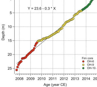
Figure 8.Depth-age model for firn cores OH-6, OH-9 and OH-10

retrieved from Laclavère Plateau. The linear relationship between depth and time was constructed based on the cores measureddexcess oscillation and a synthetically constructeddexcessfrom meteorolog-ical observations. Note that the depth axis was intentionally inverted to visualize the surface (0 m) on top.

layers (<10 mm), do not correspond to melt events and are mostly related to wind scour processes and liquid precipita-tion. Melt and crust layers do not show a clear seasonal pat-tern with relation to their time equivalent with depth. Around 70 % of melt layers counted have a width<10 mm.

4.2.2 Seasonal temperature reconstruction from stable water isotopes

The age model developed using the dexcess core

Table 4.Correlation between deuterium excess (dexcess meteo) values calculated from monthly mean meteorological data (SST and rh) and water stable isotope monthly means for all cores used in this study. Degrees of freedom (df) defined as:n−2for each correlation and cut-off frequencies for the FFT analysis are cm−1, expressing the lower and upper boundary of the integrated spectrum, respectively.

Core OH-4 OH-5 OH-6 OH-9 OH-10

Time interval Jan 2006–Jan 2009 Mar 2007–Jan 2009 Mar 2008–Jan 2010 Feb 2010–Jan 2014 Feb 2012–Jan 2015

Corr. coefficient 0.72 0.79 0.81 0.78 0.67

pvalue <0.01 <0.01 <0.01 <0.01 <0.01

df 34 21 21 47 34

Cut-off freq. (cm−1) 3.14 4.69 4.81 4.31 5.26

25.16 37.56 43.27 43.10 78.95

-3 -2 -1 0 1 2 3

Temperature anomaly (°C)

Jul Jan-09 Jul Jan-10 Jul Jan-11 Jul Jan-12 Jul Jan-13 Jul Jan-14 Jul Jan-15 Date (month-year)

-3 -2 -1 0 1 2 3

δ₁₈

O % anomaly

Normalized anomalies Temperature (°C)

δ18O‰ (positive)

δ18O‰ (negative)

Figure 9.Standardized anomalies for air (monthly mean) temperatures (solid grey colours) registered at Bellingshausen Station (BE) on King George Island and a compositeδ18O time series derived from firn cores OH-6, OH-9 and OH-10 from Laclavère Plateau. Upper translucent red (blue) boxes show period of positive (negative) anomalies, down (up) arrow shows the negative (positive) stable water isotope–temperature relationship. Both time series were detrended prior to constructing the time series of anomalies.

Calendar seasons in these latitudes do not follow regular patterns (i.e., DJF, MAM, JJA, SON), as seasonality largely depends on the sea ice cover during winter, often extending beyond calendar limits. Large sea ice extent (SIE) leads to a delayed on-set of spring conditions. In this case winter-like conditions will be extended beyond August. Restricted sea ice extent on the contrary will lead to earlier spring-like conditions (before August). Depending on such con-ditions, we defined three seasons with their corresponding δ18O–T relationship. These seasons are: (1) an austral tran-sitional season which considers the months from March to May and October–November (MAM–ON) (using precipi-tation datasets from Table 3, March 2008–2009 and Octo-ber 2014 for theδ18O–T relationship), (2) an austral winter season which considers the months from June to September (JJAS) (using precipitation datasets from June 2008 for the δ18O–T relationship, Table 3), and (3) an austral summer season which considers months from December to February (DJF) (considers precipitation datasets from December 2008 for theδ18O–T relationship). This basic classification of the seasons to describe theδ18O–T relationship does not explain all of the variability observed in the data, as some

partic-ular seasons showed variable behavior when compared to the mean seasonal behavior in the time span covered in this study. In those cases, the seasonal behavior was extended or contracted beyond the boundaries of the main season classi-fication depending on the SIE.

4.2.3 Air temperature trends at Laclavère Plateau

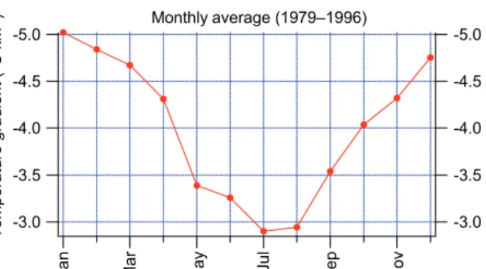
In the AP region, lapse rates change seasonally primar-ily due to variations in the presence and extent of sea ice cover which impacts thermal stability on the lower atmo-sphere. Mean seasonal lapse rates obtained in this region show a clear seasonal dependency, with the highest rates dur-ing DJF (−5.31◦_{C km}−1_{), similar values during MAM and}

SON (−4.43 and−4.06◦_{C km}−1_{respectively) and the}

low-est rates during JJA (−2.73◦C km−1) (Fig. 11).

Monthly near surface temperatures at LCL were esti-mated using a linear regression analysis based on monthly lapse rates in BE, winter SAM index and SIE from OH (Fig. 12). The resultant equation is:TLCL=(TBE−1.4)+

1.13 (Mmonth×SIEOH+Nmonth), during the months when

10

Monthly mean isotope (firn core composite)

δ18_O‰

VSMOW

dexcess‰

Month

Jul Jan Jul Jan Jul Jan Jul Jan Jul Jan Jul Jan Jul

2009 2010 201

Figure 10. (a) Monthly mean air temperature reconstruction for LCL between March 2008 and January 2015 based on air temperature

corrected by a seasonal factor and altitudinal gradient (grey line) and based on aδ18O composite time series derived from firn cores from LCL corrected by a seasonal factor (red line), respectively.(b)δ18O anddexcessmonthly mean composite time series of LCL firn cores used for the temperature reconstruction of(a).

-5.0 -5.0

-1) Monthly average (1979–1996)

Nov

Figure 11.Temperature lapse rate from sea level to 850 hPa level at Bellingshausen station (BE), King George Island, Antarctica. The data is shown as the monthly mean value of observation between 1979 and 1996 (SCAR Reference Antarctic Data for Environmental Research).

Mmonth andNMonth represent the slope and intercept of the

monthly lapse rate–SIE relationship, respectively. During the months when there is no sea ice (from October to April) the monthly temperature can be calculated from TLCL=

(TBE−1.4)+1.13×H (t ), whereH (t )is the monthly mean

lapse rate value of the month t measured in BE between 1978–1996. Considering these variables, a mean annual air temperature of −7.5◦C with a trend of −0.18◦C year−1 (statistically not significant at p=0.05) was estimated for LCL for 2009–2014. Comparatively, if only the δ18O time

series data and the isotope–T relationship are considered, a mean annual air temperature of −6.5◦C with a trend of −0.33◦C year−1(statistically not significant atp=0.05) is estimated for LCL for the same period. The correlation be-tween monthly mean temperature at LCL, estimated using theδ18O signal from firn cores andTLCLestimated using the

coupled effect of the latitude-corrected temperature record from BE, SIEOH and lapse rates from BE, have a

correla-tion coefficient ofR=0.70 (p <0.01). Both signals show a synchronous behavior, also with respect to the air temper-ature recorded at OH station. No statistically significant cor-relation was observed between coastal stations (OH and BE) temperature records and the stable water isotope composition of firn cores.

4.2.4 Accumulation rates

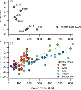
-7

Figure 12.Sea ice extent (SIE) from O’Higgins Station (OH) and

its relationship to(a)the Southern Annular Mode and(b) to the temperature gradient between sea level and 1100 m a.s.l.at the La-clavère Plateau (LCL). SIE data is from the National Snow & Ice Data Center data set (NSIDC). Sea ice extent, defined as the ex-tension of the oceanic region covered by at least 15 % ice, exhibits a negative relationship to the Southern Annular Mode between 2008 and 2014. The relationship to the temperature gradient is positive. A decreasing seasonal pattern of the temperature gradient can be observed from May to September (1979–1996).

2015 (1600 kg m−2) with an absolute minimum recorded in 2010 (1060 kg m−2) (Fig. 13a). A marked decrease was ob-served in accumulation during JJA and SON between 2008 and 2015, which could be in part responsible for the overall decreasing rates. However, this trend was found to be statis-tically non-significant (p >0.1).

The highest accumulation occurs during the MAM and SON seasons (Table 5). Accumulation rate estimations de-rived from the OH-9 and OH-10 cores for the common period 2012–2013 only differ by approximately 3 %. Other cores from the western flank of the Peninsula (OH-4, OH-5 and OH-6) show that the accumulation in 2008 (common period) depends on altitude, with increasing values from the lower region to the highest point on the LCL (Fig. 13b). The rate of increase was approximately 1500 kg m−2km−1year−1from 350 to 1130 m a.s.l.in 2008.

5 Discussion

5.1 Stable water isotope fractionation and post-depositional processes

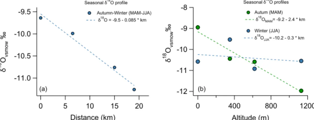
The stable water isotope composition of precipitation sam-ples from the 2008 and 2014 datasets are very similar to each other, and to firn cores from the western flank and from LCL Plateau (OH-4 to OH-10). Comparing theδ18O signal from OH-6 with data from precipitation samples at OH and with two other cores from the western side of the AP (OH-4 and OH-5) during a common period (March 2008–August 2008), aδ18O decrease of−0.085 ‰ km−1was found with increas-ing distance from the coast (Fig. 14a). The same data set was used to study theδ18O–altitude relationship. Theδ18O seasonal means show an altitude dependency that yields sea-sonal δ18O-altitude patterns. Between OH (0 m a.s.l.) and LCL (1130 m a.s.l.) during MAM, a clear decrease ofδ18O with height is observed (−2.4 ‰ km−1 withR=0.97 atp level<0.05), whereas during JJA no significant decreasing δ18O trend is observed (Fig. 14b).

Backward trajectory analysis revealed that the most fre-quent pathways for air parcels that reach the northern part of AP derive from the Bellingshausen Sea, between 55 and 60◦S throughout the year (Fig. 5). In contrast, localities fur-ther south on the AP and in West Antarctica, Ellsworth Land and coastal Ross Sea, respectively, exhibit a stronger con-tinental influence on the precipitation source, depending on seasonal and synoptic scale conditions (Thomas and Brace-girdle, 2015; Sinclair et al., 2012). The LMWL obtained from precipitation samples at OH (m=7.83) is similar to the Antarctic meteoric water line obtained by Masson-Delmotte et al. (2008) (m=7.75), and to the GMWL as presented by Rozanski et al. (1993) (m=8.13). The similarity between the slope of LMWL and GMWL indicates that the fraction-ation processes during condensfraction-ation mostly take place un-der thermodynamic equilibrium (Moser and Stichler, 1980). These results are consistent with those obtained by other au-thors for King George Island (Simões et al., 2004; Jiahong et al., 1998). Combining the stable water isotope signature of OH precipitation with time series of meteorological data rep-resentative for the conditions prevailing on the ocean near the OH station, a strong relationship with rh and SST at the mois-ture source can be derived. This relationship has been well established, especially for the coastal Antarctic region where moisture transport from the source is generally of short-range (Jouzel et al., 2013). The correlation between thedexcess of

precipitation and a theoreticaldexcess meteoderived from time

1200 1200

Accumulation (kg m-2)

2500 2500

Figure 13. (a)Accumulation rates for Plateau Laclavère during 2008–2014 estimated from the stable water isotope composition of firn

cores OH-6, OH-9 and OH-10 and their respective density profiles.(b)Accumulation variability for the west flank of the northern Antarctic Peninsula from the coast to Laclavère Plateau. Accumulation rates were derived from precipitation at O’Higgins Station at sea level and firn cores (OH-4, OH-5 and OH-6) for higher altitudes.

-11.0

Seasonalδ18_{O profile}

Autumn-Winter (MAM-JJA)

Seasonalδ18O profiles

Autum (MAM)

δ18OMAM= -9.2 - 2.4 * km

Winter (JJA)

δ18OJJA= -10.2 - 0.3 * km

(a) (b)

Figure 14.δ18O profile with relation to(a)the distance from the coast at O’Higgins Station (OH) and at different points on the west flank of the AP (6.5 km (OH-4), 15 km (OH-5) and 19 km (OH-6)) and(b)altitude at 350 m (OH-4), 620 m (OH-5) and 1130 m a.s.l.(OH-6) during autumn (MAM) (green solid dots) and winter (JJA) (blue solid dots).

an increase of contributions from other local sources (e.g., Amundsen Sea and continental conditions) to the local pre-cipitation. This has also been observed at the northern AP, where some precipitation events that exhibited a stable wa-ter isotope composition beyond the normal range for the re-gion (e.g., 20 August 2009,δ18O= −19.4 ‰), were associ-ated with uncommon sources of humidity as shown by the backward trajectory analysis.

In firn cores obtained from the AP, average values from both δ18O and δD decrease as elevation increases to LCL (1130 m a.s.l.), which supports the altitudinal isotope effect identified by Fernandoy et al. (2012a) for the region. In addi-tion, SDs of seasonal (monthly mean)δD andδ18O values of firn cores from LCL are low and similar to those of firn cores from lower altitudes. Despite the variations in isotopic com-position with height, in all firn cores theδD-δ18O co-isotopic correlation is very similar to the LMWL obtained from pre-cipitation samples at OH. This provides evidence of the uni-formity of the fractionation conditions during the condensa-tion process. Although a slight isotopic smoothing effect was distinguished between the cores (16 % after one year of de-position), the distortions caused by post-depositional effects

den-sity layers (see Sect. 4.2.1). Even though these observations are in agreement with the results obtained in this region by Fernandoy et al. (2012a) and Aristarain et al. (1990), several studies (Fernandoy et al., 2012a; Simões et al., 2004; Travas-sos and Simoes, 2004; Jiahong et al., 1998) have identified a significant melt layers in firn cores, mainly from KGI and from the western side of the AP at altitudes below 700 m a.s.l. The limited effect of post-depositional processes due to the high accumulation rates and to the ice layers reducing diffu-sion (Stichler et al., 2001), along with the high correlation be-tweendexcess meteo anddexcess cores, confirm that the isotopic

variations observed in firn core isotope records are mostly re-lated to isotopic fractionation occurring during condensation and to rh and SST conditions in the vapor source regions.

5.2 Stable water isotope and the local temperature relationship

The changing seasonal δ18O–T relationship obtained from precipitation samples shows that the relationship between air temperature and condensation temperature varies throughout the year. The strong similarity in the δ18O–T relationship during MAM and SON contrasts with the pronounced dif-ference of this relationship between DJF and JJA. This high-lights the variability of the δ18O–T relationship along the whole year at the northern AP. However, the δ18O–T cor-relations presented in this study were calculated from pre-cipitation samples of particular months and years, which can induce bias. However, it can be assumed that these datasets give an idea of the variations that can be seen in between seasons in this region. Furthermore, theδ18O–T correlations obtained for MAM and SON (0.77 and 0.61 ‰ ◦_C−1_,

re-spectively) are similar to the values obtained by other au-thors for the AP (Aristarain et al., 1986; Peel et al., 1988). Even though the dataset is capable of representing varia-tions within the time span covered by this study, it is too short to build a consistent baseline for the region. Despite the reduction of the seasonal temperature difference in coastal sites, the difference in the seasonalδ18O–T relationship sug-gests the existence of processes that disrupt the direct linkage between condensation temperature and surface air tempera-ture. The negative correlation between theδ18O signal from LCL ice cores and BE (and OH) monthly mean temperatures (Figs. 9 and 10), which is noticeable in some years during JJA, contrasts with the commonly accepted seasonal behav-ior characterized by a positive correlation betweenδ18O and surface air temperatures (Clark and Fritz, 1997). This par-ticular behavior could be related to strong variations in me-teorological conditions in the area between BE (OH) and LCL throughout the whole year. Therefore, air temperature on LCL was estimated by two independent methods: lapse rates (vertical temperature gradients) and δ18O–T equiva-lents. The best correlation between both LCL temperatures estimations was obtained when an extended seasonal behav-ior was considered (R=0.70; p <0.01). This result is in

agreement with the natural seasonal variability in high lati-tudes, where the effects of some seasons extend beyond the calendar seasonal temporal limits related to the SIE, as pre-viously explained. Without taking this seasonal variability into account would lead to a misinterpretation of the air tem-perature reconstruction for LCL, since theδ18O–T correla-tion would then be rather poor (R=0.42) and not reflect-ing the true seasonality in this region. The high similarity in the δ18O–T relationship during MAM and SON can be explained by the seasonal transition between summer and winter, when oceans surrounding the northern AP pass from ice-free to fully ice-covered conditions (or vice versa), re-spectively. Ice-free ocean conditions are related to seasonal oscillations, which are highly dependent on atmospheric cir-culation patterns. In this sense, years with a marked nega-tive SAM anomaly are associated with ice-covered sea con-ditions, whereas positive SAM phases are associated with ice-free sea conditions (Fig. 12). Other studies (Turner et al., 2016) point to a similar interaction between surface air tem-perature and SIE at AP and recognized that the SIE’s inter-annual variability is related to atmospheric modes. This sup-ports our own observations that the sea ice is important for regulation of surface air temperatures in the region.

5.3 Firn age model and accumulation rates

The stable water isotope signal obtained from firn cores shows no regularity in its seasonal behavior and lacks a clear annual oscillation pattern, likely due to the strong maritime influence (Clark and Fritz, 1997). These two criteria prevent the development of an age model by conventional annual layer counting in the isotope record (Legrand and Mayewski, 1997). In this context, thedexcess parameter represents a

ro-bust time indicator, as it has shown to be principally de-pendent on rh and SST conditions prevailing in the eastern Bellingshausen Sea where these variables are relatively sta-ble (Jouzel et al., 2013). The high correlation coefficients (and high statistical significance) obtained for the relation-ship betweendexcessanddexcess meteo, as shown in Sect. 4.2.1,

demonstrate that the method used to construct a time series is effective in dating isotope records of firn cores from the northern AP, even at a monthly resolution.

The most frequentdexcess values found in the firn cores

(3–6 ‰) are in agreement with a strong coastal influence sce-nario as determined by Petit et al. (1991), implying that the dexcess relates to rh and SST of the humidity source and not

to surface air temperature (Jouzel et al., 2013). Saigne and Legrand (1987) postulated that rh conditions prevailing at the sea surface have an important effect on thedexcesssignal

Table 5.Accumulation rates calculated for all firn cores used in this study. All rates are shown as seasonal and annual mean values with respect to the time interval covered by each core.

AP accumulation (kg m−2)

Western flank LCL

OH-4 OH-5 OH-6 OH-9 OH-10

DJF–MAM 1121

JJA–SON 1300

2006 2510

DJF–MAM 1650 >1380

JJA–SON 1300 1150

2007 2950 >2530

DJF–MAM 1130 1020 >1530

JJA–SON 770 1050 940

2008 1900 2070 >2470

DJF–MAM 1090

JJA–SON 1340

2009 2430

DJF–MAM 700

JJA–SON 360

2010 1060

DJF–MAM 680

JJA–SON 770

2011 1450

DJF–MAM 1170 1080

JJA–SON 730 690

2012 1900 1770

The irrelevance of post–depositional effects along with the flat topography on LCL suggests that the estimation of accu-mulation rates from firn cores is representative of the amount of snow originally precipitated. Moreover, the slight smooth-ing of the isotope signal after deposition, as well as the small differences in the accumulation rate observed for the com-mon time period of firn cores OH-9 and OH-10, decom-monstrates that our age model is reliable, as two different data sets yield similar estimations for a common period. The results ob-tained enable LCL to be classified as a high annual snow accumulation site (Table 5), closely following the estima-tions of other authors on King George Island dome (Bintanja, 1995; Zamoruyev, 1972; Jiahong et al., 1998) and on the AP further south of LCL (Dalla Rosa, 2013; Goodwin, 2013; van Wessem et al., 2015), of around 2000–2500 kg m−2year−1, but differs from the accumulation rate obtained by Simões et al. (2004) and Jiankang et al. (1994) on King George Island dome (600 kg m−2year−1). A seasonal accumulation bias was noted, with more favorable conditions for accumu-lation (i.e., higher precipitation amount) during autumn re-sulting from more frontal systems approaching the AP (Ta-ble 5).

5.4 Seasonal variability and disruption of atmospheric conditions

The depletion of δ18O with increasing height (altitude ef-fect) and the simultaneous increase in accumulation along the western side of AP at the LCL latitude can be explained with the help of an orographic precipitation model as proposed by Martin and Peel (1978). This model states that moist air parcels from the Southern Ocean are forced to ascend and cool down when approaching the AP due to the steep to-pography forming an orographic barrier to westerly winds. The depletion observed inδ18O reflects the strength of the fractionation process taking place within a short distance and in a low temperature environment (Fig. 15a). Therefore, the isotopic fractionation process occurring at the AP and the direct linear relationship betweenδ18O and the condensa-tion temperature enable us to study temperature behaviour with respect to altitude increase on the basis ofδ18O vari-ations (Craig, 1961). However, whereas MAM air temper-atures show a clear decrease with increasing height (atmo-spheric instability of the lower troposphere), JJA air tempera-tures exhibit an increase from sea level to 350 m a.s.l. (atmo-spheric stability). At higher altitudes, a decreasing temper-ature trend is observed (atmospheric instability). The break at 350 m a.s.l. during JJA could indicate the existence of a strong stratification within the lower troposphere on the western side of the AP. In addition, the variations in monthly mean lapse rates measured by radiosondes in BE throughout the year, provide evidence for the existence of a process that modifies the behaviour of the lower troposphere, decreasing the lapse rate (between sea level and 850 hPa) during JJA and considerably increasing it during DJF (Fig. 16).

The close linear correlation identified between lapse rate magnitude and SIE indicates that SIE is an important factor for the development of these variations, especially between May and September.

1200

750 500

250

0

LCL

OH

N25° W JJA S25° E

1200 750

500

250

0

LCL

OH

N25° W DJF S25° E

Elevation (m a.s.l.) Elevation (m a.s.l.)

Air temperature +

-Air temperature +

-1200

1000

750

500

250

0

LCL

OH

100 50 0

OH-4 OH-5

δ18_{O = -11.1 ‰}

δ18_{O = -9.6 ‰}

δ18_{O = -9.9 ‰} δ18_{O = -10.6 ‰}

N25° W S25° E

Distance from OH (km)

Elevation (m a.s.l.)

800 kg m

-2 y

-1

1900 kg m

-2 y

-1

2100 kg m

-2 y

-1

>2470 kg m

-2 y

-1

(b) (c)

(a)

Figure 15. (a)Schematic chart showing the orographic barrier effect of the AP on the stable water isotope depletion and accumulation rate at different altitudes, firn core locations (OH-4, OH-5 and OH-6) and distances from the coast (OH);(b)temperature gradient (adiabatic cooling) during DJF (summer) and sea ice free conditions;(c)inversion layer in the lower troposhere during sea ice covered conditions in JJA (winter).

Temperature Temperature

Elevation Elevation

Annual thermal oscillation LCL Annual thermal oscillation LCL

Condensation temperature Condensation temperature

Annual thermal oscillation OH Annual thermal oscillation OH

Temperature OH Temperature OH

SAM positive anomaly SAM negative anomaly

(a) (b)

Summer Autumn Winter Spring

Figure 16.Sea level to Laclavère Plateau temperature oscillation scheme during summer (DJF), autumn (MAM), winter (JJA) and spring

under(a)positive SAM anomaly conditions and(b)negative SAM anomaly conditions.

The existence of an inversion layer during the months with sea ice coverage might explain the low oscillation of monthly mean temperatures estimated at LCL compared to monthly mean air temperatures at BE (OH). The negative correlation between SAM index and SIE also seems to play an important role, as SAM positive phases enhance the transport of warm

fa-voring continental-like conditions and reducing annual mean air temperature, implying a higher temperature amplitude in BE and OH throughout the year.

The temperature time series estimated from the stable wa-ter isotope record (δ18O anddexcess) from LCL firn cores

ex-hibits a periodic (biannual) pattern, which can be linked to a similar periodical behavior observed in SAM index and in SIE. The relatively constant temperatures observed dur-ing MAM, JJA and SON in years with a positive SAM phase provide evidence that during these seasons condensa-tion is taking place at similar temperatures. Under such con-ditions (positive SAM), the low variations in the lapse rate throughout the year, along with the low thermal oscillation in BE (OH) explain the presence of a constant condensa-tion temperature, which does not differ much from air perature during DJF. Conversely, the stronger annual tem-perature oscillation observed on LCL during negative SAM phases indicates marked variations in condensation tempera-ture throughout the year.

Finally, the proposed inversion layer model (Fig. 16) ex-plains the seasonal variations observed in theδ18O–T rela-tionship of precipitation samples from OH. The distortion of the direct relationship between condensation temperature and surface air temperature by an inversion layer makes it necessary to differentiate δ18O–T relationship according to the lapse rate evolution throughout the year. In this context, MAM and SON were identified as transitional periods in the formation of the inversion layer, mainly because of the sea ice formation and retreat during these seasons. The seasonal adjustment considered to estimate LCL temperatures must be applied, because the sea ice cover varies inter-annually in its duration and extension, which in turn produces the inter-annually variable inversion layer. The proposed model for the coastal region on the western side of the AP at OH latitude, is consistent with the observations of Yaorong et al. (2003) on KGI (South Shetland Islands), where several inversion layers developed extending beyond 400 m a.s.l.

6 Conclusions

In this study, we examined one of the most complete records of recent precipitation from the northern AP, with a total of 208 single precipitation events and more than 60 m of firn cores. The firn cores retrieved in this work include the accu-mulation at the northwestern AP region between 2008 and 2014. Precipitation and firn stable water isotope composi-tions have been compared to different meteorological data sets to determine their representativeness as climate proxies for the region.

The results of our study reveal significant seasonal changes in theδ18O–T relationship throughout the year. For autumn and spring a δ18O–T ratio of 0.69 ‰ ◦C−1 (R= 0.74) was found to be most representative, whereas for win-ter and summer the δ18O–T ratio appears to be highly

de-pendent on SIE conditions. The apparent moisture source for air parcels precipitating at the northern AP is mainly located in the Bellingshausen Sea and in the southern Pacific Ocean. The transport of water vapor along these oceanic and coastal pathways exerts a strong impact on thedexcesssignal of

pre-cipitation. The comparison between thedexcess signal from

the moisture source and thedexcesssignal from firn cores has

been used successfully to date the firn cores from the north-ern AP, yielding a seven-year isotopic time series in high temporal resolution for LCL.

Based on our dating method we could define LCL as a high snow accumulation site, with a mean annual accu-mulation rate of 1770 kg m−2year−1 for the period 2006– 2014. Accumulation is highly variable from year to year, with a maximum and minimum of 2470 kg m−2(in 2008) and 1060 kg m−2 (in 2010), respectively. In addition, we identi-fied the presence of a strong orographic precipitation effect along the western side of the AP reflected by an accumulation increase with altitude (1500 kg m−2year−1km−1), as well as by the isotopic depletion of precipitation from sea level up to LCL (−2.40 ‰ km−1for autumn) and from the coast line up to the ice divide (−0.08 ‰ km−1).

The maritime regime present on the western side of the AP has a strong control on air temperatures, observed as restricted summer to winter oscillation, and is reflected in a poor seasonality of theδ18O andδD profiles in firn cores. Recent climatic conditions can be only reconstructed from δ18O time series obtained from LCL firn cores when con-sidering an inversion layer model during winter season. The strength of the inversion layer likely depends on SIE and SAM index values. Taking into account the effect of the in-version layer on the isotope–temperature relationship, we ob-serve a slight cooling trend of mean annual air temperature at LCL with an approximate rate of−0.33◦C year−1for the pe-riod sampled by the examined firn cores (2009–2014). This finding is in line with evidence from stacked meteorologi-cal record of the nearby research stations as determined by Turner et al. (2016).

Data availability. The high-resolution stable water iso-tope datasets, including firn cores and precipitation samples are available from Fernandoy et al. (2012b, 2017) via: https://doi.org/10.1594/PANGAEA.871080 and https://doi.org/10.1594/PANGAEA.871083.

Competing interests. The authors declare that they have no conflict of interest.

Acknowledgements. The present work was funded by the FONDE-CYT project 11121551 and supported by the Chilean Antarctic Institute (INACH), the Chilean Air Force and Army logistical fa-cilities. We want to show our gratitude to the Universidad Nacional Andres Bello for supporting this study. We also greatly thank our colleagues, who made field work conditions less severe, especially to Daniel Rutllant for his support in the logistical and field safety. We would like to thank all people involved in the laboratory work, especially to Ivonne Quintanilla, who carried out the sample processing at UNAB and to Johannes Freitag, for his support with the X-Ray tomography processing at AWI. Tracy Wormwood is greatly thanked for her support editing this manuscript. We highly appreciate the comments of two anonymous reviewers, who provided helpful observations that greatly contributed to improve this manuscript. Finally, we thank the dedicated work of the editor of this article Benjamin Smith.

Edited by: Benjamin Smith

Reviewed by: two anonymous referees

References

Abram, N. J., Mulvaney, R., Wolff, E. W., Triest, J., Kipfs-tuhl, S., Trusel, L. D., Vimeux, F., Fleet, L., and Arrow-smith, C.: Acceleration of snow melt in an Antarctic Peninsula ice core during the twentieth century, Nat. Geosci., 6, 404–411, https://doi.org/10.1038/ngeo1787, 2013.

Aristarain, A., Jouzel, J., and Pourchet, M.: Past Antarctic Peninsula climate (1850–1980) deduced from an ice core istope record, Cli-matic Change, 9, 69–89, 1986.

Aristarain, A., Jouzel, J., and Lorius, C.: A 400 Year Isotope record of the Antarctic Peninsula climate, Geophys. Res. Lett., 17, 2369–2372, https://doi.org/10.1029/GL017i013p02369, 1990. Aristarain, A. J., Delmas, R. J., and Stievenard, M.: Ice-Core Study

of the Link between Sea-Salt Aerosol, Sea-Ice Cover and Cli-mate in the Antarctic Peninsula Area, Climatic Change, 67, 63– 86, https://doi.org/10.1007/s10584-004-0708-6, 2004.

Bintanja, R.: The local surface energy balance of the Ecology Glacier, King George Island, Antarctica: mea-surements and modelling, Antarct. Sci., 7, 315–325, https://doi.org/10.1017/S0954102095000435, 1995.

Bromwich, D. H., Nicolas, J. P., Monaghan, A. J., Lazzara, M. A., Keller, L. M., Weidner, G. A., and Wilson, A. B.: Central West Antarctica among the most rapidly warming regions on Earth, Nat. Geosci., 6, 139–145, https://doi.org/10.1038/ngeo1671, 2013.

Cárdenas, C., Johnson, E., Fernandoy, F., Meyer, H., Cereceda, F., and Vidal, V.: Preliminary results of the superficial and sub-glacier topography survey using Radio Echo Sounding at the La Claveré Plateau, Antarctic Peninsula, SCAR Open Science Con-ference, Auckland, New Zealand, 1–3 September, 2014. Carrasco, J. F.: Decadal Changes in the Near-Surface Air

Tempera-ture in the Western Side of the Antarctic Peninsula, Atmos. Cli-mate Sci., 3, 7, https://doi.org/10.4236/acs.2013.33029, 2013. Clark, I. and Fritz, P.: Environmental Isotopes in Hydrogeology,

edited by: Stein, J., and Starkweather, A., Lewis, Boca Raton, New York, 311 pp., 1997.

Craig, H.: Isotopic variations in meteoric waters, Science, 133, 1702–1703, https://doi.org/10.1126/science.133.3465.1702, 1961.

Dalla Rosa, J.: Variabilidade da taxa de acumulação de neve no Platô Detroit, Península Antártica, M. S. thesis, Instituto de Geo-ciências, Universidade Federal do Rio Grande do Sul, Porto Ale-gre, 98 pp., 2013.

Dierssen, H. M., Smith, R. C., and Vernet, M.: Glacial melt-water dynamics in coastal melt-waters west of the Antarc-tic peninsula, P. Natl. Acad. Sci. USA, 99, 1790–1795, https://doi.org/10.1073/pnas.032206999, 2002.

Dutrieux, P., De Rydt, J., Jenkins, A., Holland, P. R., Ha, H. K., Lee, S. H., Steig, E. J., Ding, Q., Abrahamsen, E. P., and Schröder, M.: Strong Sensitivity of Pine Island Ice-Shelf Melting to Climatic Variability, Science, 343, 174–178, https://doi.org/10.1126/science.1244341, 2014.

Falk, U. and Sala, H.: Winter melt conditions of the inland ice cap on King George Island, Antarctic Peninsula, Erkunde, 69, 341– 363, https://doi.org/10.3112/erdkunde.2015.04.04, 2015. Fernandoy, F., Meyer, H., and Tonelli, M.: Stable water isotopes of

precipitation and firn cores from the northern Antarctic Peninsula region as a proxy for climate reconstruction, The Cryosphere, 6, 313–330, https://doi.org/10.5194/tc-6-313-2012, 2012a. Fernandoy, F., Meyer, H., and Tonelli, M.: High resolution stable

water isotope composition (δ18O andδD) of three firn cores and on precipitation from O’Higgins Station, Antarctica, 2008–2009, https://doi.org/10.1594/PANGAEA.871080, 2012b.

Fernandoy, F., Tetzner, D., Meyer, H., Gacitúa, G., Hoffmann, K., and Falk, U.: High resolution stable water isotope composition (δ18O andδD) of two firn cores at the northern Antarctic Penin-sula, https://doi.org/10.1594/PANGAEA.871083, 2017. Fyfe, J. C. and Saenko, O. A.: Human-Induced Change in the

Antarctic Circumpolar Current, J. Climate, 18, 3068–3073, https://doi.org/10.1175/JCLI3447.1, 2005.

Fyfe, J. C., Saenko, O. A., Zickfeld, K., Eby, M., and Weaver, A. J.: The Role of Poleward-Intensifying Winds on Southern Ocean Warming, J. Climate, 20, 5391–5400, https://doi.org/10.1175/2007JCLI1764.1, 2007.

Gille, S. T.: Decadal-Scale Temperature Trends in the Southern Hemisphere Ocean, J. Climate, 21, 4749–4765, https://doi.org/10.1175/2008JCLI2131.1, 2008.

Goodwin, B. P.: Recent Environmental Changes on the Antarctic Peninsula as Recorded in an ice core from the Bruce Plateau, PhD thesis, Graduate Program in Atmospheric Science, Ohio State University, 247 pp., 2013.