Convective instabilities in thermoviscoelastic micropolar fluids

Texto completo

(1)Vol. XIII No 1 Junio (2005) Matemáticas: 31–42. Matemáticas: Enseñanza Universitaria c °Escuela Regional de Matemáticas Universidad del Valle - Colombia. Convective instabilities in thermoviscoelastic micropolar fluids Victor A. Eremeyev. Denis A. Sukhov. Received Mar. 29, 2005. Accepted Apr. 26, 2005. Abstract Infinitesimal instabilities in plane horizontal layer of viscoelastic micropolar fluid under uniform heating are investigated. A micropolar fluid is a fluid whose particles have the six degrees of freedom of a rigid body. This model possesses couple stresses and rotational interaction of particles. Hydrodynamics of micropolar fluids has significant applications to a variety of different fields of physics and engineering (magnetohydrodynamics, tribology etc.). Like a model of liquid crystals of nematic or smectic type, the constitutive equations of viscoelastic fluids have the property of orientation elasticity. The governing equations of viscoelastic micropolar fluid of differential type are considered. The temperature effects are described by using the Oberbeck-Boussinesq approximation. The linearized initial boundary problem is deduced and its solutions are obtained. The neutral lines are presented. The material characteristics influence on the critical values of Rayleigh or Grashof numbers is investigated. It is shown that taking into account the orientation elasticity property of viscoelastic fluid leads to the increasing of critical Rayleigh or Grashof numbers. Keywords: micropolar fluid, convective instabilities, Oberbeck-Boussinesq approximation. AMSC(2000): Primary: 76E15, Secondary: 76A10, 76E06.. 1. Introduction. Models of fluids taking into account microrotations and couple stresses are known as micropolar fluids. These models ware proposed in pioneer works by E. Aero [1] and K. Eringen [2]. Within the framework of a micropolar fluid model every particle has the six degrees of freedom of a rigid body and we can take into account the rotational interaction of particles. In a micropolar fluid also exist couple stresses. Various types of constitutive equations of viscoelastic micropolar media are introduced in [3, 4, 5, 6, 7]. Extensive literature on the hydromechanics of micropolar fluids is given in the monograph [8]. The models of micropolar fluids proposed in [1]–[8] have the following characteristic property: for any equilibrium state the couple stresses vanish and we have a hydrostatic stressed state. In papers [9, 10] V. Eremeyev and L. Zubov proposed the model of viscoelastic micropolar fluid which possesses a non-hydrostatic state in that of equilibrium and has the so-called property of orientational elasticity similar to liquid crystals. For the model of viscoelastic fluid introduced in [9, 10], some static and dynamic problems have been solved, for example, viscometric flows, two-phase equilibrium, problem of capillary surface, etc..

(2) 32. V. Eremeyev and D. Sukhov. For heat convection in viscoelastic fluids some preliminary results were presented in [15, 16]. Heat convection in an infinite plane layer is a well-known example of a hydrodynamical instability, which was investigated by numerous scientists (see, for example, [11]–[14]). In this paper we present the constitutive equations for thermoviscoelastic micropolar fluids in general as well as for the special cases of a thermoelastic fluid and a thermoviscoelastic micropolar fluid of differential type. For an infinite plane layer of thermoviscoelastic micropolar fluid of differential type of complexity (1, 1) under uniform heating, we investigate convective instability for different types of boundary conditions. We determine the critical values of Rayleigh number as functions of wave number, initial curvature of microstructure and material constants. The neutral curves graphs are presented. It is shown that taking into account the property of orientation elasticity leads to increasing of the critical Rayleigh numbers. From the physical point of view it means that orientational elasticity of viscoelastic fluid has a stabilizing influence. The obtained results may be used for modelling the behavior of such complex fluids as suspensions, magnetic fluids, biological solutions, and liquid crystals. 2. Basic relations of hydromechanics of thermoviscoelastic micropolar fluid. Within the framework of a Cosserat continuum every particle has six degrees of freedom as a rigid body. The position of particle at actual time t is given by a radius-vector R(t) and its orientation is determined by a triple of orthonormal vectors D k (t) (k = 1, 2, 3) [7]. We also consider a reference configuration when the position and orientation of particles are described by vector r and directors dk (k = 1, 2, 3), respectively. Triples D k and dk produce the socalled microrotation tensor or turn-tensor H = dk ⊗ D k , which is a properly orthogonal tensor. The motion equations, the heat transfer equation and the second law of thermodynamics have the form dv , dt dω , Div M + T× + ρµ = γ dt Div T + ρm = ρ. ρ. ¡ ¢ d ε = ρs + Div h + tr T · εT + M · æT , dt ρθ. 1 d η ≥ ρs + Div h − g · h. dt θ. (1) (2) (3) (4).

(3) 33. Convective instabilities in fluids ◦. Here T and M are the Cauchy-type stress and couple stress tensors, g =∇ θ, ◦. ∇ and Div are gradient and divergence operators by using Euler description, ρ is density, m and µ are vectors of external forces and couples, γ is a scalar measure of rotational inertia, v is a linear velocity, ω is an angular velocity of triple D k : dD k / dt = ω × D k , d/ dt is a material derivative with respect to time, symbol T× denotes a vector invariant of second-rank tensor T, θ is a temperature, h is heat flux, s is a heat source density, ε and η a mass density of internal energy and entropy and I is the unit tensor. We use tensors ε and æ as measures of strain and bending strain rates. The latter are given by ◦. ε ≡∇ v + I × ω,. ◦. æ ≡∇ ω.. Following papers [9, 10] we can prove next theorem. Theorem 1. The general representation of constitutive equations of thermoviscoelastic fluid are given by £ ¤ T(t) = H1 ρ(t), B(t), Utt (s), Ltt (s), θt (s), g t (s) , ¤ £ M(t) = H2 ρ(t), B(t), Utt (s), Ltt (s), θt (s), g t (s) , ¤ £ h(t) = H3 ρ(t), B(t), Utt (s), Ltt (s), θt (s), g t (s) , (5) ¤ £ ε(t) = H4 ρ(t), B(t), Utt (s), Ltt (s), θt (s), g t (s) , ¤ £ η(t) = H5 ρ(t), B(t), Utt (s), Ltt (s), θt (s), g t (s) ,. where H1 , H2 , H3 , H4 , H5 are isotropic operators and functionals.. This theorem is a generalization of well-known Noll’s theorem on simple fluids for the case of micropolar fluids. Here we used notations which are similar to those introduced in [9],[10]. Ct (τ ) = C−1 (t) · C(τ ) is a relative strain gradient for which the actual configuration is considered as reference configuration, and configuration at time τ is considered as the actual one. Ht (τ ) = D k (t) ⊗ D k (τ ) = HT (t) · H(τ ) is a T relative microrotation tensor, h i Ut (τ ) = Ct (τ ) · Ht (τ ), Kt (τ ) = Lt (τ ) + B(t), ◦. Lt (τ )×I = − ∇ Ht (τ ) ·HTt (τ ) are relative strain measures. Here we use the following notations for pre-histories Ct (t − s) ≡ Ctt (s), θt (s) = θ(t − s), g t (s) ≡ g(t − s) etc. B and b are the tensors of curvature of microstructure in reference and actual configurations, respectively. These tensors are given by ([9],[10]) 1 b = − (∇dk ) × dk , 2. B=−. ´ 1³◦ ∇ Dk × Dk , 2. where ∇ is a nabla-operator in reference configuration. Let us consider some special cases of constitutive equations (5)..

(4) 34. V. Eremeyev and D. Sukhov. The thermoelastic micropolar fluid model is given by relations T = T(ρ, B, θ),. M = M(ρ, B, θ),. ε = ε(ρ, B, θ),. η = η(ρ, B, θ),. h = h(ρ, B, θ, g),. where the following relations hold T = ρ2. ∂ψ I − M·BT , ∂ρ. M=ρ. ∂ψ , ∂B. η=−. ∂ψ , ∂θ. here ψ ≡ ε − θη is a mass density of free energy. The heat transfer equation reduces to the form dη = Div h + ρs, dt and the Clausius-Duhem inequality reduces to the Fourier inequality ρθ. h·g ≥ 0. For the thermoelastic fluid model, energy dissipation is produced only by thermal conductivity. A simple example of a constitutive equation of elastic fluid is given by the quadratic form ¡ ¢ ¤ 1£ 2 ρψ = λtr B + µtr B · BT + νtrB2 + ρψ0 (ρ, θ), (6) 2 where λ, µ, ν are material constants, which should satisfy to the inequalities [10] 3λ + µ + ν > 0, µ + ν > 0, µ > 0, and ψ0 is a mass density of free energy when B = 0. For equation (6), we have the linear dependence of couple stresses M on B M = λItrB + µB + νBT . (7) Let us consider the thermodynamics of vicoelastic micropolar fluids of differential type. By using the approach in [17], the constitutive equations of a fluid of differential type of complexity (m, n) may be written as follows T = f1 (ρ, B, A1 . . . Am , B1 . . . Bn , θ, g), M = f2 (ρ, B, A1 . . . Am , B1 . . . Bn , θ, g), h = f 3 (ρ, B, A1 . . . Am , B1 . . . Bn , θ, g), ε = ε(ρ, B, θ),. (8). η = η(ρ, B, θ),. where f1 , f2 , f 3 are isotropic functions. Here we introduce the indifferent rate tensors An , Bn by the recurrence relations given in [10] ◦ d An + (∇ v) · An + An × ω, A0 = I, A1 = ε, dt ◦ d = Bn + (∇ v) · Bn + Bn × ω, B0 = B, B1 = æ. dt. An+1 = Bn+1.

(5) 35. Convective instabilities in fluids. A special case of (8) is a model of viscous fluid introduced by E.Aero and K.Eringen for which we have T = f1 (ρ, ε),. M = f2 (ρ, æ).. Let us consider in detail the model of micropolar fluid of differential type of complexity (1, 1). Here we have the following constitutive equations (9). T = f1 (ρ, B, ε, æ, θ, g), M = f2 (ρ, B, ε, æ, θ, g), h = f 3 (ρ, B, ε, æ, θ, g), ε = ε(ρ, B, θ), η = η(ρ, B, θ).. Stress and couple stress tensors may be written as a sum of equilibrium and dissipative parts T = TE + TD , M = M E + M D , ∂ψ ∂ψ I − ME ·BT , ME = ME (ρ, B, θ) ≡ ρ , TE = TE (ρ, B, θ) ≡ ρ2 ∂ρ ∂B TD = TD (ρ, B, θ, ε, æ, g), TD (ρ, B, θ, 0, 0, 0) = 0, MD = MD (ρ, B, θ, ε, æ, g),. MD (ρ, B, θ, 0, 0, 0) = 0.. For this case the second law (4) reduces to the dissipative inequality 1 tr(TD ·εT ) + tr(MD ·æT ) + g·h ≥ 0, θ and the heat transfer equation (3) can be transformed to the form ρθ. dη = Div h + ρs + tr(TD ·εT ) + tr(MD ·æT ). dt. (10). Let us note that the equation of thermal conductivity (10) contains summands which depend on strains. 3. Oberbeck-Boussinesq approximation for viscoelastic micropolar fluid. System of equations (1), (2), (10) describing the flow of compressible thermoviscoelastic fluid may be simplified by using some assumptions which are analogous to Oberbeck-Boussinesq approximation [11, 12, 13, 14]. Following [15, 16] we will consider incompressible fluid and will neglect the dependence of material constants on temperature and dissipation of energy due to flow. Dependence of mass density on temperature will be taken into account only in expressions of external volume forces and couples..

(6) 36. V. Eremeyev and D. Sukhov. In addition to these assumptions, we will also neglect the dependence of η on B in equation (10). For small deviations of temperature field from mean value θ◦ and by using Fourier law h = κg we can reduce equation (10) to the usual form ◦ dθ (11) = χDiv ∇ θ, dt ¯ µ ¶ κ ∂η ¯¯ where χ is the thermal conductivity coefficient χ = ◦ , Cv = . ρθ Cv ∂θ ¯θ=θ◦ Further we will use the constitutive equations in the form T = −pI + S,. ¡ ¢ S = µ 1 ε + µ 2 εT − ν 1 B + ν 2 B T · B T , T. (12). T. M = η1 æ + η2 æ + ν 1 B + ν 2 B ,. where p is a pressure and µ1 , µ2 , ν1 , ν2 , η1 , η2 are material constants. For incompressible fluid we should consider the incompressibility equation Div v = 0. 4. (13). Plane problem. In the case of plane problem an orientation of a particles is determined by one parameter. This is rotation angle α(X, Y, t) which describes the rotation of vectors D k [10]. To be specific, let us consider the rotation D 3 -axis. Thus, the vectors D k are given by D 1 = i1 cos α(X, Y, t) + i2 sin α(X, Y, t), D 2 = −i1 sin α(X, Y, t) + i2 cos α(X, Y, t),. (14). D 3 = i3 .. By using (14) the curvature tensor B is given by formula B = i1 ⊗ i3. ◦ ∂α ∂α + i2 ⊗ i 3 ≡ (∇ α) ⊗ i3 . ∂X ∂Y. (15). For the plane problem, the fields of velocity and angular velocity have a form v = v1 (X, Y, t)i1 + v2 (X, Y, t)i2 ,. ω = ω(X, Y, t)i3 ,. (16). where ω=. dα . dt. (17).

(7) 37. Convective instabilities in fluids Y. αB. −θ∗. h i2 0 i1. X αH. −h. θ∗. Figure 1: Plane layer of micropolar fluid. Thus, by using equations (14)–(17) the motion equations (1), 2 may be reduced to the form given in [10]. ∂S11 ∂S21 dv1 ∂p + + + ρm1 = ρ , ∂X ∂X ∂Y dt ∂S12 ∂S22 dv2 ∂p + + + ρm2 = ρ , − ∂Y ∂X ∂Y dt d2 α ∂M13 ∂M23 + + S12 − S21 + ρµ3 = γ 2 , ∂X ∂Y dt −. (18). where we used the following representation of external forces and couples: m = m1 i1 + m2 i2 , µ = µ3 i3 .. 5. Convective instability. Let us consider the convective instability of an infinite plane layer of thermoviscoelastic micropolar fluid of differential type of complexity (1, 1). The layer is shown on the figure 1. Here 2h is the width, −∞ < X < ∞, −h ≤ Y ≤ h. This is a generalization of well-known Rayleigh problem [11]–[14]. The temperature and the orientation of particles at the top and bottom are fixed. At the top boundary the temperature is equal to −θ∗ , and the orientation angle is equal to αB . At the bottom boundary the temperature and orientation angle are equal to θ∗ and αH , respectively. We will use the constitutive equation in form (12). For this problem, the motion equations (18), the incompressibility equa-.

(8) 38. V. Eremeyev and D. Sukhov. tion (13) and the thermal conductivity equation (11) transform to the form ∂ω ∂p + µ1 ∆v1 + (µ1 − µ2 ) − ∂X ∂Y µ µ 2 ¶ ¶ ∂α ∂ α dv1 ∂α ∂ 2 α ∂2α −ν1 2 =ρ + + , 2 2 ∂X ∂X ∂Y ∂Y ∂X∂Y dt ∂ω ∂p + µ1 ∆v2 − (µ1 − µ2 ) − − ∂X ¶ µ ¶ µ∂Y 2 ∂α ∂α ∂ 2 α ∂2α ∂ α ν1 + 2 2+ ∂Y ∂Y ∂X 2 ∂X ∂X∂Y dv2 , +ρ̃(1 + β(θ − θ◦ ))g = ρ dt µ ¶ ∂v2 ∂v1 dω dα η1 ∆ω + ν1 ∆α + (µ1 − µ2 ) − − 2ω = γ , ω= , ∂X ∂Y dt dt ∂v1 ∂v2 + = 0, ∂X ∂Y ∂θ ∂θ ∂θ + v1 + v2 = χ∆θ. ∂t ∂X ∂Y. (19). (20). (21) (22) (23). Here m1 = 0, m2 = g, g is the free fall acceleration, the dependence ◦ ρ = ρ̃(1 + β(θ − θ◦ )) is used , ρ̃ is a value of mass density ± 2 when ± θ2= θ , β is a temperature coefficient expansion (β > 0); ∆ = ∂ ∂X + ∂ ∂Y . In what follows the sign “ ˜ ” will be omitted. For the equilibrium state, the system of equations (19)–(23) has the solution which depend only on Y (p = p0 (Y ), θ = θ0 (Y ), α = α0 (Y )). That solution may be found from the equations −p00 + ρgβθ0 = 0,. α000 = 0,. θ000 = 0,. (24). taking into account the boundary conditions θ0 (h) = −θ∗ ,. θ0 (−h) = θ∗ ,. α0 (h) = αB ,. α0 (−h) = αH .. (25). Here the prime denotes the derivative with respect to Y . This initial equilibrium solution is given by θ0 = −θ∗. Y , h. α0 = −A. Y h. (A = (αB − αH )/2).. (26). The parameter A describes the initial curvature of a microstructure of fluids. Pressure distribution p0 may be determined from equation (24) taking into account relations (26). To investigate the infitesimal stability of the equilibrium solution (26) we consider a perturbed solution θ0 + τ , υ1 , υ2 , α0 + a, p0 + p, ω. The linearized form of the system (19)–(23) has the form.

(9) Convective instabilities in fluids. 39. Figure 2: Neutral curves. ∂ω ∂2a ∂υ1 ∂p + µ1 ∆υ1 + (µ1 − µ2 ) − ν1 α00 =ρ , ∂X ∂Y ∂X∂Y ∂t ∂p ∂ω − + µ1 ∆υ2 − (µ1 − µ2 ) ∂Y µ ∂X ¶ ∂2a ∂υ2 ∂2a 0 −ν1 α0 2 2 + + ρgβτ = ρ , ∂Y ∂X 2 ∂t ¶ µ ∂ω ∂υ2 ∂υ1 − − 2ω = γ , η1 ∆ω + ν1 ∆a + (µ1 − µ2 ) ∂X ∂Y ∂t ∂υ1 ∂υ2 ∂τ ∂a + α00 υ2 , + = 0, + T00 υ2 = χ∆τ. ω= ∂t ∂X ∂Y ∂t −. (27). (28). (29) (30). This a system of PDE for the small perturbations τ , υ1 , υ2 , a, p, ω. 6. Results and Conclusions. The system (27)–(30) can be investigated by the same method as in [11]. For the free boundaries the critical values of Rayleigh number are given by the following expressions obtained in [15]:.

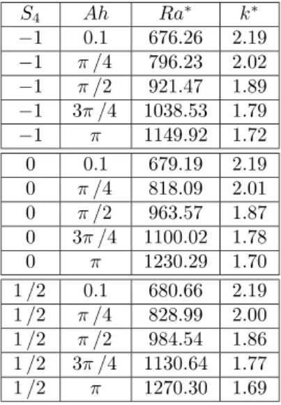
(10) 40. V. Eremeyev and D. Sukhov S4 −1 −1 −1 −1 −1 0 0 0 0 0 1 /2 1 /2 1 /2 1 /2 1 /2. Ah 0.1 π /4 π /2 3π /4 π 0.1 π /4 π /2 3π /4 π 0.1 π /4 π /2 3π /4 π. Ra∗ 676.26 796.23 921.47 1038.53 1149.92 679.19 818.09 963.57 1100.02 1230.29 680.66 828.99 984.54 1130.64 1270.30. k∗ 2.19 2.02 1.89 1.79 1.72 2.19 2.01 1.87 1.78 1.70 2.19 2.00 1.86 1.77 1.69. Table 1: Critical values of Rayleigh number and wave number (S2 = 10−6 , S3 = 10−6 (n = 1, h = 1)).. µ ¡ ¢ ¡ ¢ = S3 π 6 n6 + k 2 π 4 n4 + k 2 (2S3 + S2 S5 ) π 4 n4 + k 2 π 2 n2 + ¶Á ¡ ¢¡ ¢ ¡ 2 ¢ k 2 k 2 S3 + k 2 S2 S5 + 2S2 S4 S5 π 2 n2 + k 2 k S3 , µ ¡ ¢¡ ¢ Ra∗2 = π 6 n6 + k 2 π 4 n4 + 2k 2 + 2S4 − S1 S4 π 4 n4 + k 2 π 2 n2 + ¶ ¡ ¢¡ ¢ k 2 k 2 + 2S4 − S1 S4 π 2 n2 + k 2 × Áµ ¶ ¡ 2 2 ¢ ¡ ¢ π n + k2 k 2 π 2 n2 + k 2 + 2S4 .. Ra∗1. (31). (32). Formula (31) shows the Rayleigh numbers for a viscoelastic fluid, and formula (31) presents the Rayleigh numbers for a viscous micropolar fluid. Here we introduce the following dimensionless parameters Ra = ρgβ S3 = ν1 ρ. θ∗ h4 µ1 µ1 − µ 2 Ah , Pr = , S1 = , S2 = ν 1 ρ 2 , µ1 χ ρχ µ1 µ1. h2 (µ1 − µ2 ) h2 , S4 = , η 1 µ1 η1. S5 = Ah , S6 =. (33). µ1 γ . ρη1. By using formulas (31) and (32) we can construct the neutral curves in the plane (Ra, k), which determine the stability zone when (k < Ra(k)), and.

(11) Convective instabilities in fluids. 41. instability zone when (k > Ra(k)) for case viscoelastic and viscous fluids, respectively. For any value of n the neutral curve Ra (k) has a minimum. For all values of wave number k the minimal value of Rayleigh number corresponds to n = 1. For the viscoelastic micropolar fluid, the neutral curves are presented in figure 2, and the values of minimal Rayleigh numbers and corresponding wave numbers presented in Table 1. The case of other boundary conditions was investigated in [16] by using numerical calculations. From the obtained results we can see that taking into account the orientation elasticity property of a viscoelastic fluid leads to the increasing of critical Rayleigh numbers. From the physical point of view this means that the orientation elasticity of a viscoelastic fluid has an stabilizing influence. 7. Acknowledgements. The authors are deeply grateful to Prof. Leonid P. Lebedev for the inspiration. References [1] Aero E.L., Bulygin A.N., Kuvshinskiy E.V. Asymmetric hydromechanics (in Russian) // PMMÌ. 1965. Vol. 29. No 2. Pp. 297–308. [2] Eringen A.C. Theory of micropolar fluids // J. Math. Mech. 1966. Vol. 16. 1. P. 1–18. [3] Dinariev O. Yu., Nikolaevskiy V. N. Constitutive equations for viscoelastic media with microrotations (in Russian) // PMM. 1997. Vol. 61. 6. P. 1023–1030. [4] Allen S.J., de Silva C. N., Kline K.A. A theory of simple deformables directed fluids // Phys. Fluids. 1967. Vol. 10. 12. P. 2551–2555. [5] De Silva C. N., Kline K. A. Nonlinear constitutive equations for directed viscoelastic materials with memory // Z. Angew. Math. and Phys. 1968. Vol. 19. 1. P. 128–139. [6] Eringen A. C. Linear theory of micropolar viscoelasticity // Int. J. Eng. Sci. 1967. Vol. 5. 2. P. 191–204. [7] Eringen A. C. Microcontinuum Field Theories. I. Foundations and Solids. Berlin, et al: Springer-Verlag. 1999. [8] Migoon N. P., Prohorenko P. P. Hydrodynamics and heat transfer of gradient flows of microstructural fluid (in Russian). Minsk, 1984..

(12) 42. V. Eremeyev and D. Sukhov. [9] Zubov L. M., Eremeyev V. A. Equations of micropolar fluids // Doklady physics. 1996. Vol. 351. No 4. Pp. 472–475. [10] Eremeyev V. A., Zubov L. M. Theory of elastic and viscoelastic micropolar fluids // PMM. 1999. Vol. 63. No 5. pp. 801–815. [11] Gershuni G. Z., Zhukhovitsky E. M. Convective stability of incompressible fluid. Moscow, 1972. [12] Joseph D. D. Stability of fluid motions. I. II. Springer tracts in natural philosophy. Vol. 27, 28. Springer-Verlag: Berlin et al. 1976. [13] Hydrodynamic instabilities and the transitions to turbulence. Topics in Appl. Physics. Vol. 45. Eds. H.L.Swinney and J.P. Gollub. Springerverlag: Berlin et al. 1981. [14] Gershuni G. Z., Zhukhovitsky E. M., Nepomnjashchy A. A. Stability of convective flow. Moscow, 1989. [15] Eremeyev V. A., Sukhov D. A. Convective instability of plane layer of viscoelastic micropolar fluid with free boundaries (in Russian) //Izvestia Vuzov. Sev.-Kavk. Region. (Notices of Universities of South Russia) Natural sci. 2003. No 4. pp. 24–27. [16] Eremeyev V. A., Sukhov D. A. Convective instabilities in plane layer of viscoelastic micropolar fluid (in Russian) //Izvestia Vuzov. Sev.-Kavk. Region. (Notices of Universities of South Russia) Natural sci. 2004. Special issue. Mathematics and Mechanics of Continuum Mechanics. Pp. 101–109. [17] Truesdell C. Rational Thermodynamics. Springer-Verlag, New York, 1984. Dirección de los autores: V. A. Eremeyev, Southern Scientific Center of Russian Academy of Science, Mechanics and Mathematics Department of Rostov State University, Zorge str., 5, Rostov-on-Don, 344090, Russia, eremeyev@math.rsu.ru — D. A. Sukhov, Mechanics and Mathematics Department of Rostov State University, Zorge str., 5, Rostov-on-Don, 344090, Russia, sdrun@rambler.ru.

(13)