A radiosity based method to avoid calibration for Indoor Positioning Systems
48
0
0
Texto completo
(2) help domain experts develop services based on location faster. Keywords: Indoor positioning, Radiosity, Classification algorithm, Machine Learning. 1. Introduction Indoor positioning is a core technique for ubiquitous and pervasive computing applications. Such applications can exploit user’s position information in the services they provide to the user (Schilit et al., 1994; Abowd & Mynatt, 5. 2000; Hightower & Borriello, 2001; Kwon et al., 2005): a remote health-care monitoring system could use positioning information to recognise person’s activities and make decisions about health state (Yan et al., 2010); a position aware meeting service can provide mobile laptops with information regarding the meeting-room they are located at Castro et al. (2001); evacuation systems. 10. could provide the path to the nearest exit in an emergency case (Ingram et al., 2004). The position of the user can be estimated, for instance, in terms of latitude and longitude or at room level. The former is commonly used by guiding services where the position of the users in movement is used to guide them to their. 15. destination; the latter is used in applications where knowing the position of the user at room level is accurate enough to provide services, for example: healthcare applications, monitoring and security applications, and so on (Gu et al., 2009). Opposed to positioning systems that do not require any infrastructure to. 20. work with, like positioning systems based on the magnetic field of the Earth (Li et al., 2012), infrastructure based positioning systems need some kind of infrastructures to work with. Presented systems use cameras (Helal et al., 2009; Doukas & Maglogiannis, 2011), IR sensors (Noury et al., 2000; Demongeot et al., 2002; Costa et al., 2014); RFID technology (Calderoni et al., 2015); beacons. 25. (Tapia et al., 2012; Shirokov, 2012; Fernández-Llatas et al., 2013); and sound (Lopes et al., 2015; Cobos et al., 2016).. 2.
(3) Opportunistic WiFi signals have been extensively used as base technology for indoor positioning systems due to: a) its ubiquitous presence in urban populations; b) its relatively low cost when compared with other technologies; c) its 30. presence in most consumer mobile devices such as smart-phones, smart-watches or laptops. Different techniques have been used to exploit WiFi signals: Angle of Arrival (AoA) (Sen et al., 2013), triangulation (Lim et al., 2007) and trilateration (Mok & Retscher, 2007), being the most extended technique WiFi fingerprinting (He & Chan, 2016). The popularity of fingerprinting method is. 35. due to: a) its simplicity, b) it does not need any special hardware and, c) it is ubiquitously used. WiFi fingerprinting methods are based on the signal strength generated by a set of surrounding Wireless Access Points (WAPs) measured at different positions. This set of measures forms a WiFi map, also called radio map. Two stages are commonly used to create a WiFi map positioning system:. 40. calibration and operational stages. In the calibration stage, the set of WiFi intensity measures at different positions is taken to latter create the WiFi map. In the operational stage, a user’s device measures the WiFi signal strength of all surrounding WAPs, and this information is then used, by the positioning system, to provide an estimation of user’s position. WiFi intensity measuring is. 45. a time consuming and expensive task where different issues can happen (Casas et al., 2007; Deasy & Scanlon, 2007; Han et al., 2014), for example, any change in the environment, such as changing the location of some furniture elements, changing partition walls, changing the position of existing WAPs, deploying new WAPs, or removing existing WAPs, may degrade the positioning service, which. 50. implies the recalibration of the positioning system. Some works have appeared trying to reduce the effort needed in the calibration stage. In Gu et al. (2016) the authors reduce in a half the number of samples needed to create the WiFi map taking advantage of the hidden structure and redundancy characteristics of WiFi samples. Other works try to cope with. 55. re-calibration when changes in the environment are detected (Fet et al. (2016)), although an accuracy degradation is always present when moving furniture, new walls are lifted or removed, and so on. 3.
(4) The problem of signal propagation has been successfully solved in some other realms of science. In Physics, heat transfer between a bodies at different temper60. ature has been described using the radiosity model (Howell et al., 2010). Later, the same radiosity model was adapted and applied in Computer Graphics to model light propagation indoors for global illumination (Cohen et al., 1986; Cohen & Wallace, 2012). The definition of radiosity is: ”the radiant flux leaving a surface by unit area”. In the case of a WiFi signal, the radiant flux is the. 65. intensity of the WiFi signal. This way, existing techniques to solve the radiosity equation can be used to model the WiFi signal propagation in the presence of obstacles like walls and doors. 1.1. Motivations and Hypothesis The main motivation of this work is to use the radiosity model to describe. 70. the WiFi signal propagation indoors. This way the WiFi map used for WiFi fingerprinting indoor location systems, can be generated analytically, reducing acquisition costs in terms of time devoted to obtain the WiFi radio map, and people involved in that task. This motivation is base on the following hypothesis:. 75. 1. Given that WiFi radio waves are an electromagnetic signal, its propagation model can be simulated using the radiosity model (Cohen et al., 1986; Heckhert, 1992). 2. A WiFi radio map can be analytically obtained from the radiosity model. 3. Walls are the most important structural elements to have into account. 80. when calculating the radiosity map of the WiFi signal. Given that the WiFi radio map can be calculated analytically, the main benefits of the proposed solution are: 1. No domain expert intervention is needed in the acquisition phase, thus reducing costs.. 85. 2. The time to create the radiosity map using current CPUs is two orders of magnitude faster than manual acquisition. 4.
(5) 3. WiFi maps for new deployed WAPs, or for WAPs which changes its position, can be easily included at any time. 4. Any structural changes in the scenario can be easily taken into account to 90. re-calculate the WiFi maps. 1.2. Contributions The main goal of this work is to replace the manual acquisition of a Wifi radio map, which is a cost in term of time and people carrying out the task, by analytically calculating the WiFi radio map by means of the radiosity model.. 95. Our results show that the time consumend to analytically generate the WiFi radio map is one hundred times faster than manual acquisition. In addition, removing manual acquisition reduces the costs of creating a WiFi radio map. This main goal can be subdivided in the following contributions: 1. To model WiFi signal propagation using the radiosity technique. This. 100. way, the RSSI value is directly evaluated from the radiosity model. 2. To modify the Gaussian distribution for RSSI values to mimic its real temporal variation. 3. To compare the performance between classifiers built using real measured RSSI data, and the RSSI data calculated by the proposed radiosity model. 105. using well known Machine Learning algorithms. 4. To check if any improvement arises by mixing real measured RSSI and simulated RSSI when building a classifier. 5. To compare the impact on performance with regards to the size of the data sets used during the training phase between classifiers built using. 110. real and simulated data. To the best of our knowledge, this is the first work where the radiosity model to generate a WiFi map is applied for indoor positioning purposes. This technique would facilitate the development of new Expert Systems applications based on the users position information for ubiquitous and pervasive computing.. 115. This could relieve domain experts from the sampling task, substituting it by an 5.
(6) assistive procedure based on a radiosity WiFi map. This will allow them to focus on adding value to their applications by including the spatial context to provide better services to final users. The rest of paper is organized as follows: Section 2 presents the different 120. propagation models appeared in the literature, how WiFi maps can be used for indoor positioning, and the basics of the radiosity model. Section 3 presents the scenario used to perform the experiments, how the radiosity model has been applied to obtain the WiFi signals, the Machine Learning algorithms used, and how analytical data is perturbed to mimic the time series behaviour of real data.. 125. Section 4 presents the experimental results and discussion. Comparison with previous work, and the strengths and weaknesses of our work are presented in Section 5. Finally, the conclusions are presented in Section 6.. 2. Background and Related work First, this section presents WiFi signal propagation modelling presented in 130. previous works. Then, WiFi fingerprinting location technique is presented. Finally, a detailed description of the radiosity propagation model is presented. 2.1. WiFi signal propagation and modelling WiFi is an electromagnetic signal, which may be reflected, transmitted, absorbed and diffracted by physical objects in the scene. The intensity of an. 135. electromagnetic signal decreases with the inverse of the squared distance to the source I3D ∝. 1 r2. in a 3D open space. If the dimensions of the space reduces to. two, the signal decreases following an inverse of the distance rule I2D ∝ 1r . Decibels (dBm) are the common unit used for WiFi signal intensity, this unit takes the logarithm of the signal power, so the intensity of a WiFi signal decreases 140. with the logarithm of the distance when measured in dBm I(dBm) ∝ log r. When there are objects in the scene that interact with the electromagnetic signal, the previous rules do not work well because they do not have into account the multipath effect due to reflections on object surfaces present in the scene,. 6.
(7) absorption by objects, and diffraction on object with a size similar to the wave 145. length of the electromagnetic signal. The most common frequency used by WiFi access points (WAPs) is 2.4GHz. which corresponds to a wavelength of 12.5cm. Different models have been presented to describe the electromagnetic propagation in complex scenes. One of the most simple models is the log normal shadowing model also know as path loss model (Seybold, 2005; Ficco et al.,. 150. 2014). In this model, the different interactions with the objects in the scene are modelled as an exponent in the intensity formula, in such a way that the intensity of the electromagnetic signal decreases faster than in open space. The final result is that the intensity still remains linearly dependent with the logarithm of the distance. The main advantage of the path loss method is its simplicity.. 155. Its main drawback is the lack of accuracy. Path loss has been used in Deasy & Scanlon (2007) to calculate WiFi maps for localisation purposes, and the results presented underestimate the signal strength by up to 15 dBm. A combination of path loss WiFi modelling, Kalman filtering and RFID beacons is used in Chiou et al. (2010) to estimate the position of a user. Authors in Ali et al. (2017) use. 160. the floor plan/wall map and a path-loss model for WiFi signal propagation to estimate the WiFi signal intensity at any point on the floor plan. Ray tracing is a technique used in computer graphics to generate an image by tracing back the light rays arriving to a camera from all objects in a scene (Glassner, 1989). This model is more accurate than the path loss model because. 165. it has into account reflections, transmissions and refractions of the electromagnetic signal on objects in the scene (Kimpe et al., 1993; Yang et al., 1998). The main advantage of the ray tracing model is its accuracy when calculating the intensity of the electromagnetic signal for each point in the scene. Its main drawback is the computational time used to obtain the result. Ray tracing has. 170. been used to model WiFi signals for indoor locations in El-Kafrawy et al. (2010), Raspopoulos et al. (2012) and Ayadi et al. (2015). The radiosity method tries to directly solve the Rendering Equation (see Equation 1), which describes the interaction between an electromagnetic signal and all objects in the scene, and solves it by means of the finite elements 7.
(8) 175. technique (Zienkiewicz & Taylor, 2005). A detailed description of the radiosity method is given in Section 2.3. The ray tracing and radiosity methods are global methods because both take into account inter reflections of the electromagnetic signal between the objects present in the scene.. 180. A performance comparison of the three previously presented methods regarding its accuracy to calculate the WiFi intensity for an indoor 2D scenario is presented in Ayadi et al. (2015). The authors show that the path loss method provides the worst estimations in the scenario analysed by the authors. The most accurate method is radiosity, followed by the ray tracing method. Given. 185. the accuracy provided by the radiosity method to model WiFi signal propagation, it was chosen for testing its feasibility simulating data for developing indoor positioning services. 2.2. Indoor positioning using WiFi fingerprinting As previously mentioned, two stages are commonly used to create a WiFi. 190. fingerprinting positioning system: calibration and operational stages. In the calibration stage, the set of measures at different positions is taken to latter create the WiFi map. Lets denote this set as W = {w ~ i (~xj )} where each vector w ~ i = {s1 , s2 , ..., sk }i denotes the WiFi signal strengths for the k visible WAPs for the i-measure at position ~xj . Note that more than one measures can be. 195. taken at same position at different times. In the operational stage, a user measures the WiFi signal strength of all surrounding WAPs, and this is compared with all measures in the WiFi fingerprinting database. The estimated position for the user ~xu is such that its vector of WiFi signal intensities w ~ u minimizes some distance metrics ~xu =. 200. ~xj |min(d(w ~ i (~xj ), w ~ u )) (Torres-Sospedra et al., 2015). Machine Learning (ML) techniques have been commonly applied to estimate the position of a user based on the WiFi map information. WiFi fingerprinting positioning is a candidate problem to be solved by means of ML techniques, due to the particular characteristics of the problem: a) it is difficult to obtain an 8.
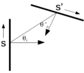
(9) 205. analytical result due to the complexity of modelling WiFi signal propagation, b) to build a computational model based on WiFi RSSI measures is a challenging problem due to its high variability over time, c) response time provided by ML algorithms is fast enough to be used in real-time applications. Extensive reviews about indoor positioning using WiFi fingerprinting can be. 210. found in Liu et al. (2007), Song et al. (2011) and He & Chan (2016). 2.3. The radiosity method The radiosity method was first developed to solve heat transfer between systems at different temperatures. Later, the radiosity method was successfully applied to solve the rendering equation, which describes the illumination for. 215. each element in a 3D scene (Cohen et al., 1986). A simplified version of such a method can be used for 2D scenes (Heckhert, 1992). For each point in a scene s, the radiosity b(s), is defined as the sum of the emitted radiation e(s), plus the reflected and transmitted radiation at such point coming from any other points in the scene. When ideal diffuse reflection. 220. and transmission is assumed, the radiosity equation is given by:. Z b(s) = e(s) + ρ(s). L. 0 0 cosθi cosθo. ds 0. 2r. 0. Z. vr b(s ) + τ (s). L. ds0. 0. cosθi cosθo0 vt b(s0 ) (1) 2r. where ρ(s) is the semicircular reflection coefficient of the diffuse material, τ (s) is the semicircular transmission coefficient of the diffuse material at point s, vr is the visibility term for reflection, vt the visibility term for transmission, and. 225. the geometric values are those shown in Figure 1. Note that for convenience, P the integral extends over all segments in the scene L = i Li The integral Equation 1 can be solved using the finite elements method, in which case, for any element in the scene i, the radiosity at this element bi can be expressed as:. bi = e i + ρ i. n X. bj Fij + τi. j=1. n X j=1. 9. bj Tij. (2).
(10) where Fij is the forward diffuse form factor given by: Z. ds0 ρh (s0 ). Fij = j 230. cosθi cosθo0 vr 2r. (3). and Tij is the backward diffuse form factor given by: Z Tij =. ds0 τh (s0 ). j. cosθi cosθo0 vt 2r. (4). Equation 2 can be written in matrix form as:. . 1 − ρ1 F1,1 − τ1 T1,1. −ρ2 F2,1 − τ2 T2,1 ... −ρn Fn,1 − τn Tn,1. .... −ρ1 F1,n − τ1 T1,n. .... −ρ2 F2,n − τ2 T2,n .... ... 1 − ρn Fn,n − τn Tn,n. . b1. . . e1. . b2 e2 = ... ... bn en. (5). Once Equation 5 is solved, the RSSI signal for any point in the scene r (RSSI(r)) can be calculated as the contribution of all radiating elements directly visible from r as:. RSSI(r) =. n X i=1. 235. bi vr 2π kr − ri k. (6). 3. Methodology This section describes the methods and materials used for data acquisition, the creation of the simulated WiFi fingerprinting data using radiosity, and the machine learning algorithms used to estimate the location of a user at room level.. 240. 3.1. Scenario description The floor plan of the scenario used to test the validity of the radiosity method applied to WiFi signals. This plan shows a corridor at the second floor of the Languages and Systems Department at Jaume I University, which dimensions. 10.
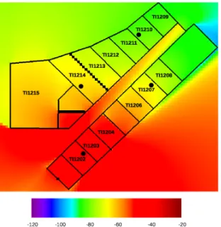
(11) are 33.0x30.5 meters. Rooms with labels TI1202 to TI1212 are teacher’s of245. fices, room TI1213 is a seminar, and rooms TI1214 and TI1215 are research laboratories. In Ayadi et al. (2015) the value for the reflection coefficient ρ = 0.1 is reported. Through experimentation, the former reported value for ρ provides the most similar results when compared with real data, so this is the value used. 250. in all performed experiments. Assuming that absorption coefficient is negligible in comparison with the transmission coefficient, the transmission coefficient was set to τ = 1 − ρ. The number of elements in the scene is a parameter fixed by the size of one of them. The lower the size of one element the more elements in the scene,. 255. and the better accuracy in the calculated radiosity map. On the contrary, the more elements in the scene, the more time spent by the algorithm to calculate the radiosity map. A size of 25cm. has been used for each element in the experiments. Four wireless access points (WAPs) were ad-hoc deployed for experimenta-. 260. tion. They are represented as black circles in Figure 2. The nominal transmission intensity was set to -20dB for all WAPs. The following assumptions were made when modelling the scenario: 1. All walls are made of the same material. 2. Doors are made of the same material as walls.. 265. 3. There is neither specular transmission nor reflection. 4. The absorption coefficient is negligible. With the former assumptions, the radiosity equation in Equation 1 was applied to simulate WiFi signal propagation. 3.2. The radiosity method. 270. The rendering Equation 1 was solved using the finite elements technique and matrix Equation 5, with the assumptions presented in Section 3.1. Four WiFi maps were calculated, one for each one of the WAPs showed in Figure 2.. 11.
(12) Once the radiosity was calculated for each structural element, the RSSI signal for each point in the space was calculated using Equation 6. Figure 2 shows 275. the calculated WiFi map for the WAP located at office TI1202. Similar results were obtained for the other three WAPs, which are not shown for brevity. 3.3. Machine Learning Techniques The problem of estimating, at room level {c1 = T I1202, ...cn = T I1215}, a user’s position p ∈ C ≡ {c1 , ..., cn } given the vector w ~ = {s1 , s2 , ..., sk } of. 280. measured RSSI of the k surroundings WAPs, can be seen as a supervised classification problem f (w ~ = {s1 , s2 , ..., sk }) ⇒ ci . A complete description of Machine Learning techniques dealing with classification problems can be found in (Alpaydin, 2004; Marsland, 2015). A data set is needed to train a classifier. For indoor positioning purposes,. 285. each element in the data set is made of the vector w ~ j of RSSI measures and the room cj where those were measured {w ~ j , cj }, also called the radio map. In this work, two different training data sets were used to build a classifier: a) the data set with measured RSSI, hereinafter named the real classifier; and b) simulated data provided by the generated radiosity maps, hereinafter named the simulated. 290. classifier. This way, the performance of the two classifiers can be compared to test the validity of our initial hypothesis. Six well known and widely used classifiers (Kotsiantis (2007); Wu et al. (2008)) were used to compare the performance of real and simulated classifiers: 1. Bayes Network (BN): probabilistic graphical classification algorithm based. 295. on the Bayes’ rule (Pearl (2014)). 2. K Nearest Neighbours (KNN): finds the k elements in the training set nearest to test sample, and estimates the class of the test sample based on the minimum distance. Euclidean distance was used, and a value for k = 1 (Sillverman et al. (1951)).. 300. 3. Multi Layer Perceptron (MLP): a Neural Network with one or more hidden layers. Eight neurons were used in the only hidden layer, which corresponds to the experssion. #attributes+#classes 2. 12. (Cybenko (1989))..
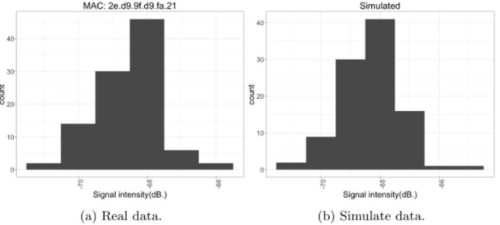
(13) 4. Random Forest (RF): ensemble of decision trees classifier. One hundred trees were used (Breiman, 2001). 305. 5. Support Vector Machine (SVM): Separates two classes with an hyperplane with maximal margins. Radial Basis Function were used as kernel (Cortes & Vapnik, 1995). 6. Sequential Minimal Optimization (SMO): Originally developed for training SVM, it can be also used as a classifier (Platt, 1998).. 310. An ensemble classifier was also used for performance comparison (Alpaydin, 2004). This ensemble is made up of the former six classifiers, and estimates user’s position based on the sum of probably estimates of the results of all six classifiers. Experimental results using the seven classification algorithms are presented. 315. in Section 4.3. 3.4. Time series of simulated data Gaussian distribution is commonly used to characterize the WiFi signal intensity measured in a single position (Kaemarungsi & Krishnamurthy, 2004). Although a more correct characterization implies a mixture of Gaussian distri-. 320. butions (Kaemarungsi & Krishnamurthy, 2012), a single Gaussian distribution can be used as a first approximation. Figure 3 (left) shows the distribution of a WiFi signal for 100 samples. Moreover, WiFi signal varies along the time for any fixed point in space. This is mainly due to interferences with other electromagnetic signals, fluctuations. 325. of the emitting WAP and in the receiver’s antenna, just to cite a few. Figure 4 (a) shows a time series of a WiFi signal for a single position. When simulating data it is important to mimic both behaviours: simulated data must follow a Gaussian distribution, and its time series must mimic real data. To mimic the first behaviour, the mean and standard deviation were esti-. 330. mated from real data. Maximum Likelihood was used to fit real measured RSSI to a Gaussian distribution. For the particular set of real data showed in Figure 3 (left) the fit provides µ = −68.54 ± 0.09 and σ = 0.94 ± 0.07. Figure 3 (right) 13.
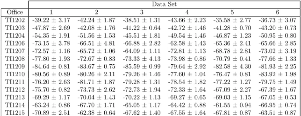
(14) shows the histogram obtained for a set of 100 samples randomly generated using a Gaussian distribution with the former values for the parameters. Although 335. both histograms may seem similar, they do not describe the RSSI variation along the time, Figures 4 (a) and (b), show the time series of real data and simulated data following a Gaussian distribution with the mean and standard deviation values provided when adjusting the real data. It can be noted that although both data sets have the same Gaussian distribution, the time series. 340. are quite different. For real data the same WiFi signal intensity might remain unchanged for some consecutive measures. On the contrary, the simulated data changes almost with any new simulated measure. To mimic the second behaviour, an inertial factor was introduced. This factor keeps the last simulated intensity for a random number of following mea-. 345. sures. From real data, it was estimated that each measure keeps unchanged 80% of samples, on average. Figures 4 (b) and (c) show a time series of simulated data without inertia (b) and with inertia (c). Through experimentation, it has been check that the resulting distribution followed a Gaussian distribution. Ten different experiments were performed. For each experiment, 1000 samples fol-. 350. lowing a Gaussian distribution with µ = −68.54 and σ = 0.94 were generated, and then the inertial factor was applied. The p-value for a Chi-Squared test was greater than 0.99 in all ten experiments. So, with a high confidence level, it can be concluded that the resulting data series followed a Gaussian distribution.. 4. Experimental Results 355. This sections firstly presents how data sets were acquired, and their main statistics. Then, simulated data using radiosity is presented, and compared with the real data. Also, the classification performance when using real versus simulated data is compared. Following, the same classifiers were used to study the performance when mixing real and simulated data. Finally, the performance. 360. dependency with regards to the number of samples used in the training stage is compared for the cases of real and simulated classifiers.. 14.
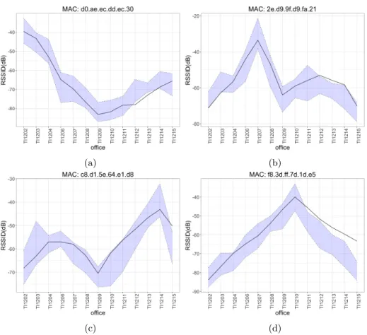
(15) 4.1. Real data Six data sets were acquired in six different days. The week of the day, and the time of the day were different for all six data sets. One hundred measures 365. were acquired at each office, while standing up at the centre of the room. All experiments were carried out by the same person, and with the same smart-phone: Aquaris BQ M5, Android version: 6.0.1. Table 1 summarizes the statistics for the RSSI of the WAP with MAC d0:ae:ec:dd:ec:30. Tables for other MACs are omitted for brevity. The average time to acquire one data set was 120 minutes.. 370. The mean value of standard deviation for all data acquired including all WAPs was σ = 1.64, its maximum value was σmax = 3.14 and its minimum value was σmin = 0.90. 4.2. Simulated data Following the assumptions made in Section 3.1, and having ρ = 0.1 (reflec-. 375. tion coefficient) and τ = 0.9 (transmission coefficient), four radiosity maps were generated, one of them for each WAP deployed. Figure 2 shows the radiosity map for WAP located at office TI1202. The location of all WAPs is showed in Figure 2. An Intel i7-4790 CPU at 3.60 GHz with 16 GB RAM and Linux Mint 18.2. 380. was used to generate radiosity maps. The average time consumed to generate a single radiosity map was 70 seconds. To generate a radiosity map is more than 100 times faster that to acquire real data. Moreover, the radiosity map provides data for each point in the floor plan, while manual acquisition provides data only for a set of selected points in the floor plan.. 385. The RSSI value read from the radiosity map for each position at the centre of the room office was altered following the scheme presented in Section 3.4. The value used to alter the simulated data was σ = 2.02. Figure 5 shows the RSSI for the simulated values compared with the RSSI for real data. Each of the four sub-figures shows the data for a particular. 390. WAP, identified by its MAC address. For each sub-figure, each point in the dashed upper strip-line is the maximum of RSSI plus the standard deviation 15.
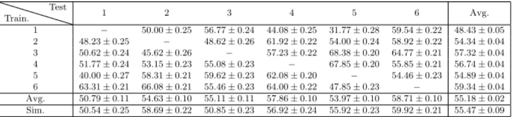
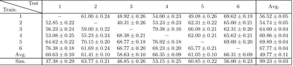
(16) for the corresponding office. For example, point for office TI1202 in Figure 5-a is the maxs∈S {RSSI + σs } for elements in first row of Table 1, where S ≡ {1, 2, 3, 4, 5, 6}. In the same way, each point in the dashed lower strip-line 395. is the minimum of RSSI minus the standard deviation for the corresponding office mins∈S {RSSI − σs }. Remarkably, more than 80% of simulated RSSI values, for the four studied WAPs, are between these two limits. 4.3. Performace comparison The particular classification task used to compare the performance was a. 400. challenging problem, only four characteristics were used to estimate the label (office ID) in a 13 classes classification problem. It was expected that, even using real data to build the classifier, the performance will be moderate. But the objective of the comparison it was to asses how good are the results provided by the simulated classifiers compared with the real ones, not to asses the. 405. performance of the simulated classifiers themself. The following procedure was used to compare the classification performance using real classifiers and simulated classifiers: first, seven classifiers were built using one data set as training data (data sets: 1 to 6 for real data, and Sim. for simulated data); second, data sets 1 to 6 were used for testing. Tables 2-7 show. 410. the percentage of correct estimates for each classification algorithm used. For each row, the data set on the left most column was used as training data when building the classifier, and all data sets in other columns were used to test the classifiers. The elements in the diagonal, which corresponds to the result when the training and test data sets are the same, are omitted. The row with label. 415. Avg. corresponds to the averages of all six elements in the same column (same testing data set). The row with label Sim. corresponds to the classifier built using simulated data. The last column shows the performance average for all five data sets used for testing with the same training set. Table 2 shows the results when using a Bayes Network classifier, in all cases,. 420. the classifier built using simulated data never gave the worst result. The percentage of correctly classified samples for the simulated classifier is always above 50% 16.
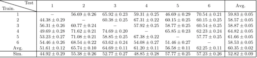
(17) of correctly classified rooms, far away from a random guess. The performance differences, for the same test set, between classifiers using real and simulated data ranges between 0.25 and 4.26. The mean performance for all tested data 425. set in the case of real classifier was 55.18 (see Table 9), and the mean performance for the simulated classifier was 55.47, which is remarkably close to the real performance. Table 3 shows the results when using a KNN classifier. The simulated classifier gave the worst results for 4 of 6 tests sets, but in one case only, the. 430. performance was below 50% of correctly classified rooms. The performance differences between classifiers, for the same test set, using real and simulated data ranges between 1.17 and 11.92. The mean performance for the real classifier was 60.35, and the mean performance for the simulated classifier was 52.82. Table 4 shows the results when using a Multi Layer Perceptron. Again, in. 435. this case the classifier built using simulated data gave the worst results in 3 of 6 tests sets, but in one case only the performance was below 50% of correctly classfied rooms. The performance differences between classifiers, for the same test set, using real and simulated data ranges between 0.20 and 23.25. The mean performance for the real classifier was 62.40, and the mean performance. 440. for the simulated classifier was 53.00. Table 5 shows the results when using a Random Forest classifier. Remarkably, the classifier built when using simulated data gave the best results in 2 of 6 test sets, and never gave the worst result. The performance differences between classifiers, for the same test set, using real and simulated data ranges between. 445. 0.72 and 13.31. The mean performance for the real classifier was 53.84, and the mean performance for the simulated classifier was 57.86, which is remarkably close to the real performance. In this case, the mean performance of the simulated classifier was higher than the real classifier. Table 6 shows the results when using a Sequential Minimal Optimization. 450. classifier. The simulated classifier gave the worst results in 2 of 6 test sets, but in these two case the percentage of correctly classified rooms were above 60%. The performance differences between classifiers, for the same test set, using real 17.
(18) and simulated data ranges between 6.57 and 11.91. The mean performance for the real classifier was 73.22, and the mean performance for the simulated 455. classifier was 66.31. Table 7 shows the results when using a Support Vector Machine classifier. The simulated classifier never gave the worst result using this classifier. The performance differences between classifiers using real and simulated data ranges between 0.53 and 12.37 for the same test set. The mean performance for the. 460. real classifier was 68.98, and the mean performance for the simulated classifier was 64.95. Table 8 shows the results when using an ensemble classifier using the results of all six previous classifiers. The ensemble built using simulated data gave the worst result in one case only. The percentage of correctly classified data. 465. was 68.92% which means 2 of 3 correctly classified rooms on average. The performance differences between classifiers using real and simulated data ranges between 2.55 and 11.13 for the same test set. The mean performance for the real classifier was 70.36, and the mean performance for the simulated classifier was 65.96.. 470. Table 9 shows a summary comparing the average performance between real and simulated classifiers, and its differences. The last row in the Table 9 shows the difference between the averaged values. The biggest difference was 7.35 for KNN classifier and the smallest was -4.02 for the RF classifier, which remarkably performs better, averaging all results, for the simulated classifier. In the case. 475. of the Ensemble classifier, the mean performance value is 65.96 ± 0.08, namely, the Ensemble correctly classifies 2 of 3 test samples. The difference in the mean, between real and simulated classifiers, for the Ensemble classifier is 4.40, this shows that simulated data generated using the radiosity algorithm provides accurate results when used to build indoor positioning classifiers.. 480. 4.4. Combining real and simulated data In this section, the classifier performance when real measures are combined with simulated data to create the classifiers is analysed. The objective of these 18.
(19) tests were to assess if it is possible to improve the performance of already built classifiers by adding new simulated data to the original training data set, without 485. taking new real samples. For each experiment, one hundred simulated samples were added to one hundred real measures, so the total number of elements in the training set was two hundred. After that, the performance was measured following the same procedure than in Section 4.3. For the sake of brevity, average results are. 490. presented only. Table 10 shows a summary comparing the performance between real and simulated classifiers, and their differences. All results improved with regards those presented in Table 9, even the difference becomes narrower in all cases but for the Bayes Network classifier. In the case of the Ensemble classifier, the. 495. mean performance value was 78.18 ± 0.07, so more than 3 of 4 test samples were correctly classified on average. The difference regarding the real Ensemble classifier was 1.89 ± 0.08, that is less than two percentage points. 4.5. Leave-one-out performance comparison This set of experiments compares the results when building each classifier. 500. leaving one of the six data sets out for training, and using the left data set for testing. Five hundred measures were used to build each classifier. In the case of the simulated classifier, five hundred simulated measures were generated following the scheme presented in Section 3.4. Table 11 shows the leave-one-out experimental results. The percentage of correctly classified rooms for the sim-. 505. ulated classifier is always below the corresponding real classifier. The smallest difference between real (78.08%) and simulated (76.77%) classifiers was for the Random Forest classifier when testing set was number 6, which is less than two percentage points. Although there is an improvement when more data is used to build real clas-. 510. sifiers, there is not a clear improvement in the case of the simulated classifiers. In the next section it is studied how generalization improves with regards the size of the training data. 19.
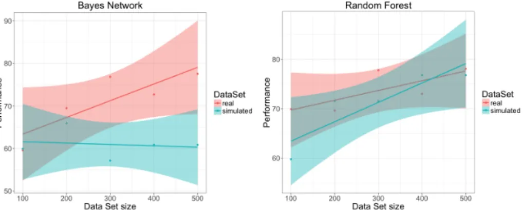
(20) 4.6. Generalization with regards the number of samples in the training set The performance of a classifier depends on how well it is classifying new data, 515. in other words, how well it generalises when classifying new data. It is desirable that a learning algorithm will improve its performance with experience, namely, when the number of samples in the training set increases (Flach, 2012). The results presented in this section study how performance behaves when increasing the size of the training data set for real and simulated classifiers.. 520. Performance was compared when the number of training data was increased in one hundred new samples at each steps. In the case of real measurements, this was done just summing up a new real dataset to the previous training data. In the case of the simulated data, this were done generating a new simulated data set of one hundred samples, and adding it to the previous simulated data set.. 525. Results are shown in Table 12. The first column in this table refers to the size of the training data set, 1 means that only the samples in data set 1 were used to train the classifier, 12 means that samples in data sets 1 and 2 were used to train the classifier, and so on. Sim100 refers to a training data set composed on 100 simulated samples, Sim200 refers to a training data set composed on 200. 530. simulated samples, and so on. Taken the results in Table 12 there is no clear increase in performance when increasing the number of samples used in the training phase. However, if results for 100 samples and 500 samples are compared, only, there is a clear improvement for all classifiers.. 535. Figure 6 shows the particular cases for the Bayes Network and MLP classifiers. Bayes Network real classifier clearly follows a linear trend with positive slope regarding the size of the training data set. On the contrary, when using simulated samples, the trend exhibits a negative slope. In the case of the Random Forest classifier, real and simulated training data sets show a linear trend. 540. with positive slope when increasing the size of the data sets used in training stage, even the performance in the simulated case exhibits a bigger value for the slope. Although for some classifiers the performance improves when more samples are used in the training data set, this is not true in general. 20.
(21) 5. Discussion 545. The radio propagation model for indoor positioning presented in Deasy & Scanlon (2007) uses an empirical model based on the radio signal absorption by walls, the final absorption is obtained by counting the number of walls between the radio signal emitter and the observer, no inter-reflexion between walls are taken into account as the radiosity model presented in this paper do. The work. 550. in Han et al. (2014) presents an ubiquitous application for indoor navigation based on the interpolation of the WiFi RSSI signal between sample points; although this approach reduces the number of samples, and so the acquisition time, they still need some manual data acquisition. The same interpolation approach, but using a different technique, is presented in Gu et al. (2016) where. 555. they use a sparsity rank singular value decomposition to interpolate the WiFi RSSI signal at sampled points; again, although the number of sampled points is reduced their solution still needs some manual data acquisition. In Ayadi et al. (2015) the authors compare three different empirical models to study its appropriateness to ITU accuracy statistics recommendation for 2.4 GHz indoor test. 560. environment, but they do not apply their conclusions to develop any application in the expert systems realm. In this paper, the data provided by the radio map obtained with the radiosity model is used to develop a positioning system based on machine learning algorithms commonly used in the expert system realm. Compared with previous works, the main strength of this work is to com-. 565. pletely remove the manual acquisition step in the offside development of a positioning system, which in turn dramatically reduces the time needed to develop them. Also, when the radio WiFi map is generated any number of sample points can be taken to build machine learning algorithms. Any change in the environment, as an addition or removal of a WiFi access point, or a relocation of an. 570. access point, can be easily taken into account by building a new WiFi radio map for the access point involved. To have the complete WiFi radio map might be a valuable tool for domain experts developing expert systems applications based on indoor location information.. 21.
(22) The weaknesses of the presented work rely on the information needed to 575. create the radiosity map. It is required to have a precise floor map of the area, on the contrary, the radiosity generated map could be degraded. To have an accurate measure of the material absorption for the walls is also important to obtain an accurate radiosity map.. 6. Conclusions 580. In this work, how to reduce or even completely remove the calibration stage when building radio maps for indoor positioning has been explored. The proposed alternative to sampling RSSI WiFi signal at different positions to create the radio map, is to calculate this radio map based on the radiosity model, which describes radio signal propagation for indoor scenarios in the presence of obsta-. 585. cles like walls and doors. Regarding the time consumed to generate simulated data sets, it is one hundred times faster to generate data using the radiosity model than with manual acquisition. Moreover, the radiosity map provides the RSSI level for each point in the floor plan, while manual acquisition provides data for the sampled point only. Additionally, removing manual data acquisition. 590. reduces the cost for creating WiFi maps. This might easy the use of positioningbased Expert Systems development in big scenarios where WiFi sampling is a high time consuming task (Casas et al. (2007); Han et al. (2014)). Experimental results, based on well known machine learning algorithms commonly used in expert systems development, showed that the accuracy of the presented method. 595. is close to manual acquisition of data. Even in those cases where positioning systems are already working, the results presented in this paper show that to add new samples from the radiosity map to real samples improves the final accuracy in almost 10% for the case of an ensemble of classifiers. The implication for already developed ubiquitous and pervasive applications based on position-. 600. ing information is that it might be possible to improve their performances by adding new radiosity simulated data. As short-term future work, we plan to adapt our radiosity implementation. 22.
(23) code to take profit of the power of modern GPUs, which could reduce the time consumed to generate the radiosity map two orders of magnitude. This improve605. ment would provide near real-time tools for Expert Systems applications based on positioning information; as an example, this could allow domain experts to accurately fix the position of WiFi access points to maximize the accuracy of the positioning algorithms. In the medium term, we plan to extend the radiosity algorithm to three dimensions, this could provide better radiosity maps at the. 610. expenses of more calculus; again, we could use a GPU implementation of the 3D radiosity to reduce processing time. As stated in one result of this work, to mix real and radiosity information improves the accuracy of positioning algorithms, so in the medium term we plan to use a robot to take real samples without any manual intervention. Finally, in the long term, and for those cases where the. 615. floor map is not available, we plan to use artificial intelligence algorithms, based on the information provided by radiosity map, to estimate the position of the walls in the area of interest.. Acknowledgements This work has been partially funded by the Spanish Ministry of Economy 620. and Competitiveness through the “Proyectos I + D Excelencia” programme (TIN2015-70202-P) and by Jaume I University “Research promotion plan 2017” programme (UJI-B2017-45).. References Abowd, G. D., & Mynatt, E. D. (2000). Charting past, present, and future 625. research in ubiquitous computing. ACM Trans. Comput.-Hum. Interact., 7 , 29–58. URL: http://doi.acm.org/10.1145/344949.344988. doi:10.1145/ 344949.344988. Ali, M. U., Hur, S., & Park, Y. (2017). Locali: Calibration-free systematic localization approach for indoor positioning. Sensors, 17 . URL: http://. 630. www.mdpi.com/1424-8220/17/6/1213. doi:10.3390/s17061213. 23.
(24) Alpaydin, E. (2004). Introduction to Machine Learning. MIT Press. Ayadi, M., Torjemen, N., & Tabbane, S. (2015). Two-dimensional deterministic propagation models approach and comparison with calibrated empirical models. IEEE Transactions on Wireless Communications, 14 , 5714–5722. 635. Breiman, L. (2001). Random forests. Machine Learning, 45 , 5–32. URL: http: //dx.doi.org/10.1023/A:1010933404324. doi:10.1023/A:1010933404324. Calderoni, L., Ferrara, M., Franco, A., & Maio, D. (2015). Indoor localization in a hospital environment using random forest classifiers. Expert Systems with Applications, 42 , 125 – 134. URL: http://www.sciencedirect.. 640. com/science/article/pii/S0957417414004497. doi:http://dx.doi.org/ 10.1016/j.eswa.2014.07.042. Casas, R., Cuartielles, D., Marco, A., Gracia, H. J., & Falco, J. L. (2007). Hidden issues in deploying an indoor location system. IEEE Pervasive Computing, 6 , 62–69.. 645. Castro, P., Chiu, P., Kremenek, T., & Muntz, R. (2001). A probabilistic room location service for wireless networked environments. In Ubicomp 2001: Ubiquitous Computing (pp. 18–34). Springer. Chiou, Y.-S., Wang, C.-L., & Yeh, S.-C. (2010). An adaptive location estimator using tracking algorithms for indoor wlans.. 650. Wireless Networks,. 16 , 1987–2012. URL: http://dx.doi.org/10.1007/s11276-010-0240-8. doi:10.1007/s11276-010-0240-8. Cobos, M., Perez-Solano, J. J., Belmonte, Ó., Ramos, G., & Torres, A. M. (2016). Simultaneous ranging and self-positioning in unsynchronized wireless acoustic sensor networks. IEEE Transactions on Signal Processing, 64 , 5993–. 655. 6004. Cohen, M. F., Greenberg, D. P., Immel, D. S., & Brock, P. J. (1986). An efficient radiosity approach for realistic image synthesis. IEEE Computer graphics and Applications, 6 , 26–35. 24.
(25) Cohen, M. F., & Wallace, J. R. (2012). Radiosity and realistic image synthesis. 660. Elsevier. Cortes, C., & Vapnik, V. (1995). Support-vector networks. Machine Learning, 20 , 273–297. URL: http://dx.doi.org/10.1007/BF00994018. doi:10. 1007/BF00994018. Costa, N., Domingues, P., Fdez-Riverola, F., & Pereira, A. (2014). A mobile. 665. virtual butler to bridge the gap between users and ambient assisted living: A smart home case study. Sensors, 14 , 14302–14329. Cybenko, G. (1989). Approximation by superpositions of a sigmoidal function. Mathematics of Control, Signals and Systems, 2 , 303–314. URL: http://dx. doi.org/10.1007/BF02551274. doi:10.1007/BF02551274.. 670. Deasy, T. P., & Scanlon, W. G. (2007). Simulation or measurement: The effect of radio map creation on indoor wlan-based localisation accuracy. Wireless Personal Communications, 42 , 563–573. URL: http://dx.doi.org/10.1007/ s11277-006-9211-x. doi:10.1007/s11277-006-9211-x. Demongeot, J., Virone, G., Duchne, F., Benchetrit, G., Herv, T., Noury, N., &. 675. Rialle, V. (2002). Multi-sensors acquisition, data fusion, knowledge mining and alarm triggering in health smart homes for elderly people. Comptes Rendus Biologies, 325 , 673 – 682. Longevite et vieillissement. Doukas, C., & Maglogiannis, I. (2011). Emergency fall incidents detection in assisted living environments utilizing motion, sound, and visual perceptual. 680. components. Information Technology in Biomedicine, IEEE Transactions on, 15 , 277–289. El-Kafrawy, K., Youssef, M., El-Keyi, A., & Naguib, A. (2010). Propagation modeling for accurate indoor wlan rss-based localization. In 2010 IEEE 72nd Vehicular Technology Conference - Fall (pp. 1–5). doi:10.1109/VETECF.. 685. 2010.5594108.. 25.
(26) Fernández-Llatas, C., Benedi, J.-M., Garcı́a-Gómez, J. M., & Traver, V. (2013). Process mining for individualized behavior modeling using wireless tracking in nursing homes. Sensors, 13 , 15434–15451. Fet, N., Handte, M., & Marrn, P. J. (2016). An approach for autonomous 690. recalibration of fingerprinting-based indoor localization systems. In 2016 12th International Conference on Intelligent Environments (IE) (pp. 24–31). doi:10.1109/IE.2016.13. Ficco, M., Esposito, C., & Napolitano, A. (2014). Calibrating indoor positioning systems with low efforts. IEEE Transactions on Mobile Computing, 13 , 737–. 695. 751. doi:10.1109/TMC.2013.29. Flach, P. (2012). Machine learning: the art and science of algorithms that make sense of data. Cambridge University Press. Glassner, A. S. (1989). An introduction to ray tracing. Elsevier. Gu, Y., Lo, A., & Niemegeers, I. (2009). A survey of indoor positioning systems. 700. for wireless personal networks. IEEE Communications surveys & tutorials, 11 , 13–32. Gu,. Z.,. (2016).. Chen,. Z.,. Zhang,. Y.,. Zhu,. Y.,. Lu,. M.,. & Chen,. Reducing fingerprint collection for indoor localization.. A.. Com-. puter Communications, 83 , 56 – 63. URL: http://www.sciencedirect. 705. com/science/article/pii/S0140366415003643. doi:http://dx.doi.org/ 10.1016/j.comcom.2015.09.022. Han, D., Jung, S., Lee, M., & Yoon, G. (2014). Building a practical wi-fibased indoor navigation system. IEEE Pervasive Computing, 13 , 72–79. doi:10.1109/MPRV.2014.24.. 710. He, S., & Chan, S. H. G. (2016). Wi-fi fingerprint-based indoor positioning: Recent advances and comparisons. IEEE Communications Surveys Tutorials, 18 , 466–490. doi:10.1109/COMST.2015.2464084.. 26.
(27) Heckhert, P. S. (1992). Radiosity in flatland. In Computer Graphics Forum (pp. 181–192). Wiley Online Library volume 11. 715. Helal, A., Schmalz, M., & Cook, D. J. (2009). Smart home-based health platform for behavioral monitoring and alteration of diabetes patients. Journal of Diabetes Science and Technology, (pp. 141–148). Hightower, J., & Borriello, G. (2001). Location systems for ubiquitous computing. Computer , 34 , 57–66. doi:10.1109/2.940014.. 720. Howell, J. R., Menguc, M. P., & Siegel, R. (2010). Thermal radiation heat transfer . CRC press. Ingram, S., Harmer, D., & Quinlan, M. (2004). Ultrawideband indoor positioning systems and their use in emergencies. In Position Location and Navigation Symposium, 2004. PLANS 2004 (pp. 706–715). IEEE.. 725. Kaemarungsi, K., & Krishnamurthy, P. (2004). Properties of indoor received signal strength for wlan location fingerprinting. In Mobile and Ubiquitous Systems: Networking and Services, 2004. MOBIQUITOUS 2004. The First Annual International Conference on (pp. 14–23). IEEE. Kaemarungsi, K., & Krishnamurthy, P. (2012). Analysis of wlans received signal. 730. strength indication for indoor location fingerprinting. Pervasive and mobile computing, 8 , 292–316. Kimpe, M., Bohossian, V., & Leib, H. (1993). Ray tracing for indoor radio channel estimation. In Proceedings of 2nd IEEE International Conference on Universal Personal Communications (pp. 64–68 vol.1). volume 1. doi:10.. 735. 1109/ICUPC.1993.528349. Kotsiantis, S. (2007). Supervised machine learning: a review of classification techniques. Informatica, 31 , 249–269. Kwon, O., Yoo, K., & Suh, E. (2005).. Ubidss:. a proactive intel-. ligent decision support system as an expert system deploying ubiqui740. tous computing technologies.. Expert Systems with Applications, 28 , 27.
(28) 149 – 161. URL: http://www.sciencedirect.com/science/article/pii/ S0957417404000983. doi:https://doi.org/10.1016/j.eswa.2004.08.007. Li, B., Gallagher, T., Dempster, A. G., & Rizos, C. (2012). How feasible is the use of magnetic field alone for indoor positioning? In 2012 International 745. Conference on Indoor Positioning and Indoor Navigation (IPIN) (pp. 1–9). doi:10.1109/IPIN.2012.6418880. Lim, C.-H., Wan, Y., Ng, B.-P., & See, C.-M. S. (2007). A real-time indoor wifi localization system utilizing smart antennas. IEEE Transactions on Consumer Electronics, 53 .. 750. Liu, H., Darabi, H., Banerjee, P., & Liu, J. (2007). Survey of wireless indoor positioning techniques and systems. IEEE Transactions on Systems, Man, and Cybernetics, Part C (Applications and Reviews), 37 , 1067–1080. Lopes, S. I., Vieira, J. M., Reis, J., Albuquerque, D., & Carvalho, N. B. (2015). Accurate smartphone indoor positioning using a wsn infrastructure and non-. 755. invasive audio for tdoa estimation. Pervasive and Mobile Computing, 20 , 29–46. Marsland, S. (2015). Machine learning: an algorithmic perspective. CRC press. Mok, E., & Retscher, G. (2007). Location determination using wifi fingerprinting versus wifi trilateration. Journal of Location Based Services, 1 , 145–159.. 760. Noury, N., Herve, T., Rialle, V., Virone, G., Mercier, E., Morey, G., Moro, A., & Porcheron, T. (2000). Monitoring behavior in home using a smart fall sensor and position sensors. In Microtechnologies in Medicine and Biology, 1st Annual International, Conference On. 2000 (pp. 607–610). Pearl, J. (2014). Probabilistic reasoning in intelligent systems: networks of. 765. plausible inference. Morgan Kaufmann. Platt, J. (1998). Sequential Minimal Optimization: A Fast Algorithm for Training Support Vector Machines. Technical Report. 28.
(29) Raspopoulos, M., Laoudias, C., Kanaris, L., Kokkinis, A., Panayiotou, C. G., & Stavrou, S. (2012). 3d ray tracing for device-independent fingerprint-based 770. positioning in wlans. In 2012 9th Workshop on Positioning, Navigation and Communication (pp. 109–113). doi:10.1109/WPNC.2012.6268748. Schilit, B., Adams, N., & Want, R. (1994). Context-aware computing applications. In 1994 First Workshop on Mobile Computing Systems and Applications (pp. 85–90). doi:10.1109/WMCSA.1994.16.. 775. Sen, S., Lee, J., Kim, K.-H., & Congdon, P. (2013). Avoiding multipath to revive inbuilding wifi localization. In Proceeding of the 11th Annual International Conference on Mobile Systems, Applications, and Services MobiSys ’13 (pp. 249–262). New York, NY, USA: ACM. URL: http://doi.acm.org/10.1145/ 2462456.2464463. doi:10.1145/2462456.2464463.. 780. Seybold, J. S. (2005). Introduction to RF propagation. John Wiley & Sons. Shirokov, I. (2012). Precision indoor objects positioning based on phase measurements of microwave signals. In S. Chessa, & S. Knauth (Eds.), Evaluating AAL Systems Through Competitive Benchmarking. Indoor Localization and Tracking (pp. 80–91). Springer Berlin Heidelberg volume 309 of Communi-. 785. cations in Computer and Information Science. Sillverman, B., Jones, M., Fix, E., & Hodges, J. (1951). An important contribution to nonparametric discriminant analysis and density estimation. International Statistical Review , 57 , 233–247. Song, Z., Jiang, G., & Huang, C. (2011). A survey on indoor positioning tech-. 790. nologies. In Theoretical and Mathematical Foundations of Computer Science (pp. 198–206). Springer. Tapia, D. I., Garcia, O., Alonso, R. S., Guevara, F., Catalina, J., Bravo, R. A., & Corchado, J. (2012). The n-core polaris real-time locating system at the evaal competition. In S. Chessa, & S. Knauth (Eds.), Evaluating AAL Sys-. 795. tems Through Competitive Benchmarking. Indoor Localization and Tracking 29.
(30) (pp. 92–106). Springer Berlin Heidelberg volume 309 of Communications in Computer and Information Science. Torres-Sospedra, J., Montoliu, R., Trilles, S., Belmonte, O., & Huerta, J. (2015). Comprehensive analysis of distance and similarity measures for wi-fi 800. fingerprinting indoor positioning systems. Expert Systems with Applications, 42 , 9263 – 9278. URL: http://www.sciencedirect.com/science/article/ pii/S0957417415005527. doi:http://doi.org/10.1016/j.eswa.2015.08. 013. Wu, X., Kumar, V., Quinlan, J. R., Ghosh, J., Yang, Q., Motoda, H., McLach-. 805. lan, G. J., Ng, A., Liu, B., Philip, S. Y. et al. (2008). Top 10 algorithms in data mining. Knowledge and information systems, 14 , 1–37. Yan, H., Huo, H., Xu, Y., & Gidlund, M. (2010). Wireless sensor network based e-health system-implementation and experimental results. IEEE Transactions on Consumer Electronics, 56 , 2288–2295.. 810. Yang, C.-F., Wu, B.-C., & Ko, C.-J. (1998). A ray-tracing method for modeling indoor wave propagation and penetration. IEEE Transactions on Antennas and Propagation, 46 , 907–919. doi:10.1109/8.686780. Zienkiewicz, O. C., & Taylor, R. L. (2005). The finite element method for solid and structural mechanics. Butterworth-heinemann.. 30.
(31) Figure 1: Geometry for the surface elements S and S’. The length of element S’ is Li .. 31.
(32) Figure 2: RSSI map generated using the radiosity method. WAP was located at office TI1202. Colours represents intensities in dBm. Black points show position of the four WAPs used in the experiments.. 32.
(33) (a) Real data.. (b) Simulate data.. Figure 3: Histograms of the WiFi signal intensity for real data (left), and simulated data (right), for 100 samples. The values for simulated data were µ = −68.54, σ = 0.94.. 33.
(34) (a) Real data.. (b) Simulated data.. (c) Simulated inertia.. Figure 4: Temporal series of real data (a), simulated data (b), and simulated data with hysteresis. For simulated data the normal distribution was generated taken µ = −68.54 and σ = 0.94. The inertia factor keeps the current data 80% of times on average.. 34.
(35) (a). (b). (c). (d). Figure 5: These figures show the measure intensity for each of the four WAP identified by their MAC address, compared with the simulated data. The upper limit of the light violet ribbon represents the maximum intensity measured in all six data sets. The lower limit of the ribbon represents the minimum. The solid line shows the RSSI signal for simulated data. On the horizontal axes, offices are sorted by code.. 35.
(36) Figure 6: Overfitting comparison between classifiers built with real and simulated data.. 36.
(37) Table 1: Statistics (mean ± standard deviation) for the RSSI of WAP with MAC address d0.ae.ec.dd.ec.30. Each row shows the data for an office, and for one of the six data sets acquired. Unit is dB. Data Set Office TI1202 TI1203 TI1204 TI1206 TI1207 TI1208 TI1209 TI1210 TI1211 TI1212 TI1213 TI1214 TI1215. 1 -39.22 ± -47.87 ± -54.35 ± -73.15 ± -72.57 ± -77.80 ± -84.64 ± -80.56 ± -76.20 ± -75.70 ± -69.29 ± -63.24 ± -70.89 ±. 3.17 2.69 1.91 3.78 1.16 1.93 0.81 0.89 2.63 0.82 1.17 0.86 2.51. 2 -42.24 ± -42.08 ± -51.56 ± -66.51 ± -65.72 ± -72.67 ± -83.67 ± -80.26 ± -81.71 ± -73.73 ± -70.04 ± -67.70 ± -62.38 ±. 1.87 1.76 1.53 4.81 1.06 0.83 0.75 2.11 1.87 2.62 1.43 1.71 0.64. 3 -38.51 ± -41.22 ± -45.51 ± -66.88 ± -64.09 ± -73.33 ± -85.59 ± -79.26 ± -79.28 ± -72.73 ± -70.22 ± -65.05 ± -67.62 ±. 1.31 0.64 1.81 2.82 1.11 4.13 0.99 1.46 1.31 1.94 1.13 1.17 1.40. 37. -43.66 -42.72 -49.54 -62.58 -72.81 -73.98 -79.64 -77.60 -78.54 -72.33 -69.27 -64.42 -67.55. 4 ± ± ± ± ± ± ± ± ± ± ± ± ±. 2.23 1.46 1.46 1.43 1.13 0.86 2.92 1.04 1.82 1.64 0.65 0.88 1.64. -35.58 -41.28 -46.87 -65.36 -68.78 -70.79 -82.58 -76.47 -77.22 -67.09 -69.03 -61.55 -67.81. 5 ± ± ± ± ± ± ± ± ± ± ± ± ±. 2.77 0.70 1.23 2.41 2.81 0.41 4.30 0.81 1.27 2.27 1.15 0.94 0.87. -36.73 -43.20 -50.95 -65.66 -73.02 -77.66 -81.93 -83.92 -79.75 -67.39 -67.05 -66.95 -63.51. 6 ± ± ± ± ± ± ± ± ± ± ± ± ±. 3.07 0.73 0.80 2.85 3.19 1.33 2.25 1.98 1.49 1.67 0.53 0.74 0.87.
(38) Table 2: Performance comparison results for the real and simulated Bayes Network. Test Train. 1 2 3 4 5 6 Avg. Sim.. 1. 2. 3. 4. 5. 6. Avg.. − 48.23 ± 0.25 50.62 ± 0.24 51.77 ± 0.24 40.00 ± 0.27 63.31 ± 0.21 50.79 ± 0.11 50.54 ± 0.25. 50.00 ± 0.25 − 45.62 ± 0.26 53.15 ± 0.23 58.31 ± 0.21 66.08 ± 0.21 54.63 ± 0.10 58.69 ± 0.22. 56.77 ± 0.24 48.62 ± 0.26 − 55.08 ± 0.23 59.62 ± 0.23 55.46 ± 0.23 55.11 ± 0.11 50.85 ± 0.23. 44.08 ± 0.25 61.92 ± 0.22 57.23 ± 0.22 − 62.08 ± 0.20 64.00 ± 0.22 57.86 ± 0.10 56.92 ± 0.24. 31.77 ± 0.28 54.00 ± 0.24 68.38 ± 0.20 67.85 ± 0.20 − 47.85 ± 0.23 53.97 ± 0.10 55.92 ± 0.23. 59.54 ± 0.22 58.92 ± 0.22 64.77 ± 0.21 55.85 ± 0.21 54.46 ± 0.23 − 58.71 ± 0.10 59.92 ± 0.21. 48.43 ± 0.05 54.34 ± 0.04 57.32 ± 0.04 56.74 ± 0.04 54.89 ± 0.04 59.34 ± 0.04 55.18 ± 0.02 55.47 ± 0.09. 38.
(39) Table 3: Performance comparison results for the real and simulated K Nearest Neighbours. Test Train. 1 2 3 4 5 6 Avg. Sim.. 1. 2. 3. 4. 5. 6. Avg.. − 44.38 ± 0.29 56.31 ± 0.26 49.69 ± 0.28 53.23 ± 0.27 54.46 ± 0.26 51.61 ± 0.12 44.92 ± 0.29. 56.69 ± 0.26 − 60.77 ± 0.24 71.62 ± 0.21 71.08 ± 0.21 68.54 ± 0.22 65.74 ± 0.10 55.38 ± 0.26. 65.92 ± 0.23 60.38 ± 0.25 − 74.69 ± 0.20 58.85 ± 0.25 63.62 ± 0.24 64.69 ± 0.11 52.77 ± 0.27. 59.31 ± 0.25 67.31 ± 0.22 57.92 ± 0.25 − 67.38 ± 0.22 54.08 ± 0.27 61.20 ± 0.11 48.85 ± 0.28. 46.69 ± 0.29 60.15 ± 0.25 58.77 ± 0.25 65.85 ± 0.23 − 51.46 ± 0.27 56.58 ± 0.11 57.77 ± 0.25. 70.54 ± 0.21 60.15 ± 0.25 60.54 ± 0.25 62.23 ± 0.24 57.77 ± 0.25 − 62.25 ± 0.11 57.23 ± 0.26. 59.83 ± 0.05 58.57 ± 0.05 58.87 ± 0.05 64.82 ± 0.05 61.66 ± 0.05 58.53 ± 0.05 60.35 ± 0.02 52.82 ± 0.09. 39.
(40) Table 4: Performance comparison results for the real and simulated Multi Layer Perceptron. Test Train. 1 2 3 4 5 6 Avg. Sim.. 1. 2. 3. 4. 5. 6. Avg.. − 52.85 ± 0.22 56.23 ± 0.24 53.08 ± 0.25 64.62 ± 0.22 76.38 ± 0.18 60.63 ± 0.10 37.38 ± 0.29. 61.00 ± 0.24 − 59.00 ± 0.22 55.23 ± 0.24 70.15 ± 0.20 61.69 ± 0.24 61.41 ± 0.10 63.77 ± 0.21. 48.92 ± 0.26 40.31 ± 0.26 − 68.38 ± 0.21 68.77 ± 0.18 66.77 ± 0.20 58.63 ± 0.10 46.85 ± 0.26. 54.00 ± 0.23 53.23 ± 0.23 79.38 ± 0.16 − 76.92 ± 0.18 68.23 ± 0.20 66.35 ± 0.09 53.15 ± 0.25. 49.08 ± 0.26 62.31 ± 0.22 66.08 ± 0.21 62.00 ± 0.21 − 65.77 ± 0.21 61.05 ± 0.10 60.85 ± 0.22. 69.62 ± 0.19 65.00 ± 0.21 62.31 ± 0.20 65.62 ± 0.21 69.00 ± 0.20 − 66.31 ± 0.09 56.00 ± 0.23. 56.52 ± 0.05 54.74 ± 0.05 64.60 ± 0.04 60.86 ± 0.04 69.89 ± 0.04 67.77 ± 0.04 49.77 ± 0.11 99.23 ± 0.03. 40.
(41) Table 5: Performance comparison results for the real and simulated Random Forest. Test Train. 1 2 3 4 5 6 Avg. Sim.. 1. 2. 3. 4. 5. 6. Avg.. − 41.46 ± 0.24 43.54 ± 0.25 61.08 ± 0.23 35.92 ± 0.27 70.46 ± 0.19 50.49 ± 0.11 43.38 ± 0.24. 54.77 ± 0.24 − 50.69 ± 0.23 58.00 ± 0.23 56.15 ± 0.21 53.85 ± 0.25 54.69 ± 0.10 68.00 ± 0.19. 54.62 ± 0.24 50.54 ± 0.24 − 79.62 ± 0.16 45.92 ± 0.23 51.77 ± 0.23 56.49 ± 0.10 55.77 ± 0.20. 37.08 ± 0.28 58.31 ± 0.22 54.85 ± 0.22 − 59.31 ± 0.22 62.00 ± 0.21 54.31 ± 0.10 61.92 ± 0.22. 37.46 ± 0.28 53.62 ± 0.25 51.38 ± 0.21 52.92 ± 0.23 − 51.31 ± 0.24 49.34 ± 0.10 58.31 ± 0.21. 69.92 ± 0.17 47.62 ± 0.23 51.69 ± 0.23 63.62 ± 0.19 55.69 ± 0.23 − 57.71 ± 0.10 59.77 ± 0.21. 50.77 ± 0.05 50.31 ± 0.05 50.43 ± 0.05 63.05 ± 0.04 50.60 ± 0.05 57.88 ± 0.04 53.84 ± 0.02 57.86 ± 0.09. 41.
(42) Table 6: Performance comparison results for the real and simulated Sequential Minimal Optimization. Test Train. 1 2 3 4 5 6 Avg. Sim.. 1. 2. 3. 4. 5. 6. Avg.. − 64.69 ± 0.25 71.85 ± 0.25 69.08 ± 0.25 72.00 ± 0.25 83.08 ± 0.25 76.14 ± 0.11 60.23 ± 0.25. 68.15 ± 0.25 − 65.85 ± 0.25 81.00 ± 0.25 77.23 ± 0.25 81.08 ± 0.25 78.58 ± 0.11 66.77 ± 0.25. 70.38 ± 0.25 68.08 ± 0.25 − 84.08 ± 0.25 84.69 ± 0.25 71.62 ± 0.25 79.33 ± 0.11 61.08 ± 0.25. 57.46 ± 0.25 70.23 ± 0.25 81.38 ± 0.25 − 76.31 ± 0.25 61.00 ± 0.25 73.76 ± 0.11 60.38 ± 0.25. 57.38 ± 0.25 63.92 ± 0.25 72.08 ± 0.25 82.31 ± 0.25 − 67.69 ± 0.25 73.56 ± 0.11 77.15 ± 0.25. 88.62 ± 0.25 80.08 ± 0.25 78.15 ± 0.25 75.46 ± 0.25 71.69 ± 0.25 − 81.86 ± 0.11 72.23 ± 0.25. 68.40 ± 0.05 69.40 ± 0.05 73.86 ± 0.05 78.39 ± 0.05 76.38 ± 0.05 72.89 ± 0.05 73.22 ± 0.02 66.31 ± 0.10. 42.
(43) Table 7: Performance comparison results for the real and simulated Support Vector Machine. Test Train. 1 2 3 4 5 6 Avg. Sim.. 1. 2. 3. 4. 5. 6. Avg.. − 48.08 ± 0.28 58.31 ± 0.25 67.62 ± 0.22 65.62 ± 0.23 81.08 ± 0.17 64.14 ± 0.10 51.77 ± 0.27. 57.23 ± 0.26 − 60.08 ± 0.25 72.23 ± 0.21 86.08 ± 0.15 66.31 ± 0.23 68.39 ± 0.09 68.92 ± 0.22. 68.00 ± 0.22 79.08 ± 0.18 − 91.31 ± 0.12 70.31 ± 0.21 66.08 ± 0.23 74.96 ± 0.08 66.77 ± 0.23. 41.46 ± 0.30 74.92 ± 0.20 73.92 ± 0.20 − 77.23 ± 0.19 67.85 ± 0.22 67.08 ± 0.09 59.23 ± 0.25. 52.77 ± 0.27 65.77 ± 0.23 65.69 ± 0.23 76.62 ± 0.19 − 57.54 ± 0.26 63.68 ± 0.10 73.62 ± 0.20. 83.23 ± 0.16 64.15 ± 0.23 75.31 ± 0.19 81.54 ± 0.17 74.00 ± 0.20 − 75.65 ± 0.09 69.38 ± 0.22. 60.54 ± 0.05 66.40 ± 0.04 66.66 ± 0.04 77.86 ± 0.04 74.65 ± 0.04 67.77 ± 0.04 68.78 ± 0.02 64.95 ± 0.09. 43.
(44) Table 8: Performance comparison results for the real and simulated Ensemble. Test Train. 1 2 3 4 5 6 Avg Sim.. 1. 2. 3. 4. 5. 6. Avg.. − 54.69 ± 0.21 64.08 ± 0.20 68.00 ± 0.21 66.62 ± 0.21 81.77 ± 0.16 67.03 ± 0.09 57.69 ± 0.22. 59.23 ± 0.21 − 62.38 ± 0.20 72.69 ± 0.18 84.92 ± 0.16 69.69 ± 0.19 69.78 ± 0.08 67.23 ± 0.18. 67.46 ± 0.19 65.69 ± 0.19 − 89.46 ± 0.14 72.92 ± 0.18 68.31 ± 0.18 72.77 ± 0.08 63.46 ± 0.20. 52.00 ± 0.22 77.38 ± 0.18 76.77 ± 0.17 − 77.54 ± 0.17 68.85 ± 0.18 70.51 ± 0.08 60.62 ± 0.21. 50.54 ± 0.23 69.38 ± 0.19 71.38 ± 0.18 79.23 ± 0.17 − 63.08 ± 0.20 66.72 ± 0.08 77.85 ± 0.18. 84.00 ± 0.15 70.38 ± 0.19 72.08 ± 0.18 77.62 ± 0.17 72.69 ± 0.18 − 75.35 ± 0.08 68.92 ± 0.19. 62.65 ± 0.04 67.50 ± 0.04 69.34 ± 0.04 77.40 ± 0.03 74.94 ± 0.04 70.34 ± 0.04 70.36 ± 0.02 65.96 ± 0.08. 44.
(45) Table 9: Average performance values and difference between real and simulated classifiers for tested classifiers.. Real Sim. Diff.. BN 55.18 ± 0.02 55.47 ± 0.09 −0.29 ± 0.11. KNN 60.35 ± 0.02 52.82 ± 0.09 7.53 ± 0.11. MLP 62.40 ± 0.02 53.00 ± 0.10 9.40 ± 0.12. RF 53.84 ± 0.02 57.86 ± 0.09 −4.02 ± 0.11. 45. SMO 73.22 ± 0.02 66.31 ± 0.10 6.91 ± 0.12. SVM 68.98 ± 0.02 64.95 ± 0.09 4.03 ± 0.11. Ensemble 70.36 ± 0.02 65.96 ± 0.08 4.40 ± 0.09.
(46) Table 10: Average performance for classifiers built with 100 real samples plus 100 simulated samples compared with simulated classifiers built with 200 simulated samples. Differences are shown in the last row.. 100Real+100Sim. 200Sim. Diff.. BN 75.75 ± 0.01 72.37 ± 0.07 3.38 ± 0.08. KNN 71.45 ± 0.02 70.05 ± 0.09 1.40 ± 0.10. MLP 74.28 ± 0.01 68.91 ± 0.08 5.37 ± 0.09. 46. RF 73.93 ± 0.02 75.17 ± 0.09 −1.24 ± 0.11. SMO 79.73 ± 0.02 77.86 ± 0.10 1.87 ± 0.12. SVM 77.94 ± 0.01 77.66 ± 0.07 0.28 ± 0.08. Ensemble 80.07 ± 0.01 78.18 ± 0.07 1.89 ± 0.08.
(47) Table 11: Leave-one-out comparison result for real and simulated classifiers. Train. 12345 Sim500 12346 Sim500 12356 Sim500 12456 Sim500 13456 Sim500 23456 Sim500. Test 6 6 5 5 4 4 3 3 2 2 1 1. Bayes Net. 77.54 ± 0.16 60.85 ± 0.22 65.23 ± 0.19 59.46 ± 0.23 76.46 ± 0.16 53.85 ± 0.24 69.46 ± 0.18 60.77 ± 0.23 71.92 ± 0.17 62.69 ± 0.21 71.54 ± 0.19 49.31 ± 0.26. KNN 72.38 ± 0.21 57.69 ± 0.25 68.15 ± 0.22 55.92 ± 0.26 66.23 ± 0.23 49.00 ± 0.28 69.15 ± 0.22 51.85 ± 0.27 65.08 ± 0.23 51.77 ± 0.27 55.54 ± 0.26 43.46 ± 0.29. MLP 81.38 ± 0.15 53.31 ± 0.25 71.15 ± 0.19 50.46 ± 0.26 68.54 ± 0.18 52.15 ± 0.26 65.46 ± 0.20 53.54 ± 0.26 75.23 ± 0.16 44.46 ± 0.27 75.31 ± 0.18 39.85 ± 0.29. 47. RF 78.08 ± 0.15 76.77 ± 0.18 69.69 ± 0.19 63.23 ± 0.20 62.62 ± 0.20 55.15 ± 0.22 76.31 ± 0.17 60.00 ± 0.22 63.46 ± 0.21 60.23 ± 0.19 67.85 ± 0.20 56.46 ± 0.22. SMO 88.92 ± 0.25 72.46 ± 0.25 80.54 ± 0.25 74.38 ± 0.25 85.69 ± 0.25 60.54 ± 0.25 83.92 ± 0.25 62.92 ± 0.25 84.85 ± 0.25 67.15 ± 0.25 80.08 ± 0.25 58.38 ± 0.25. SVM 89.15 ± 0.13 71.85 ± 0.21 76.08 ± 0.19 62.77 ± 0.24 86.77 ± 0.14 62.15 ± 0.24 81.62 ± 0.17 70.92 ± 0.21 76.38 ± 0.19 66.31 ± 0.23 74.23 ± 0.20 52.69 ± 0.27. Ensemble 89.08 ± 0.13 72.15 ± 0.18 75.69 ± 0.16 73.31 ± 0.19 82.31 ± 0.14 60.31 ± 0.21 83.77 ± 0.15 65.46 ± 0.20 71.77 ± 0.16 61.00 ± 0.20 77.46 ± 0.18 58.08 ± 0.22.
Figure

+7
Documento similar