Changes in beach shoreline due to sea level rise and waves under climate change scenarios: application to the Balearic Islands (western Mediterranean)

Texto completo

(1)Nat. Hazards Earth Syst. Sci., 17, 1075–1089, 2017 https://doi.org/10.5194/nhess-17-1075-2017 © Author(s) 2017. This work is distributed under the Creative Commons Attribution 3.0 License.. Changes in beach shoreline due to sea level rise and waves under climate change scenarios: application to the Balearic Islands (western Mediterranean) Alejandra R. Enríquez1 , Marta Marcos1 , Amaya Álvarez-Ellacuría2 , Alejandro Orfila1 , and Damià Gomis1 1 IMEDEA, 2 SOCIB,. Universitat de les Illes Balears – CSIC, Esporles, Spain Balearic Islands Coastal Observing and Forecasting System, Palma de Mallorca, Spain. Correspondence to: Alejandra R. Enríquez ([email protected]) Received: 4 November 2016 – Discussion started: 12 December 2016 Revised: 17 May 2017 – Accepted: 1 June 2017 – Published: 7 July 2017. Abstract. This work assesses the impacts in reshaping coastlines as a result of sea level rise and changes in wave climate. The methodology proposed combines the SWAN and SWASH wave models to resolve the wave processes from deep waters up to the swash zone in two micro-tidal sandy beaches in Mallorca island, western Mediterranean. In a first step, the modelling approach has been validated with observations from wave gauges and from the shoreline inferred from video monitoring stations, showing a good agreement between them. Afterwards, the modelling set-up has been applied to the 21st century sea level and wave projections under two different climate scenarios, representative concentration pathways RCP45 and RCP85. Sea level projections have been retrieved from state-of-the-art regional estimates, while wave projections were obtained from regional climate models. Changes in the shoreline position have been explored under mean and extreme wave conditions. Our results indicate that the studied beaches would suffer a coastal retreat between 7 and up to 50 m, equivalent to half of the present-day aerial beach surface, under the climate scenarios considered.. 1. Introduction. Rising sea levels represent one of the major threats for coastal regions, causing submersion, erosion and increased vulnerability to extreme marine events, among other negative impacts (Nicholls and Cazenave, 2010). It is expected that such effects will be aggravated in the coming decades as sea level rise accelerates in response to global warming (Church. et al., 2013) and coastal population and development grow (Hanson et al., 2011). Several studies have related coastline retreat during the last decades with sea level rise (e.g. Feagin et al., 2005; FitzGerald et al., 2008), although other relevant processes have also been identified (Passeri et al., 2015). These include oceanic forcing by wave climate and storms, direct or indirect human actions (e.g. mining activities or fluid extraction), and local features such as coastal morphology (Cazenave and Le Cozannet, 2014). Coastline retreat has important environmental impacts but also socio-economic implications as it affects population, infrastructures and assets. The impact of sea level rise in the shoreline position has therefore become a subject of increasing concern, particularly in densely populated regions with high urban development. This is the case for many Mediterranean regions, whose economies, which constitute about 14 % of the total gross domestic product of the EU (Eurostat, 2011), largely rely on tourism based on beach and other seaside recreational activities. Thus, sea level rise and its potential impacts are key factors that must be incorporated in coastal risk management and climate change adaptation measures. In this paper, we investigate the shoreline changes in two anthropized micro-tidal sandy beaches located in Mallorca (Balearic Islands, western Mediterranean Sea) are investigated. Here, the shoreline is defined as the water–land interface of the beach, i.e. the limit of the swash zone. The potential impacts of a shoreline retreat would increase the vulnerability of the nearshore infrastructures. In addition, both are typical tourism-oriented beaches in urban environments. Published by Copernicus Publications on behalf of the European Geosciences Union..

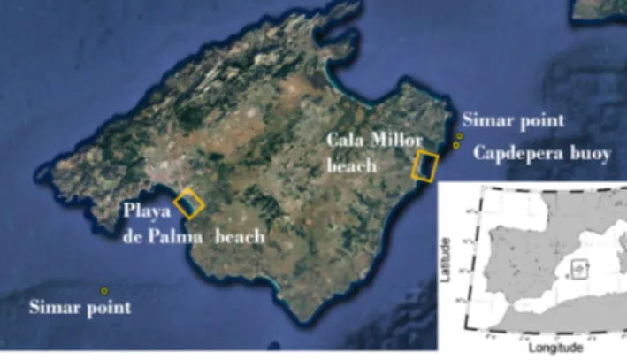
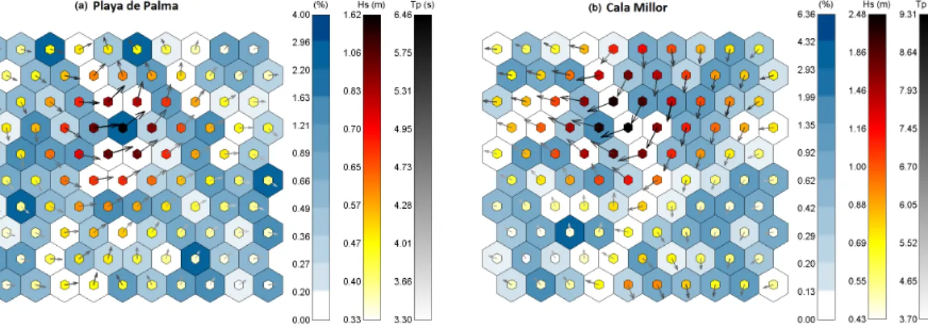
(2) 1076. A. R. Enríquez et al.: Changes in beach shoreline under climate change scenarios. of the Mediterranean region, so their reduction or disappearance would be detrimental for the local economies. The impact of sea level rise along sandy coastlines consists of two processes, namely inundation and erosion. Increased sea levels allow waves and surges to act at higher levels landward in the beach profile, increasing erosion rates (Zhang et al., 2004). However, in this study the beach erosion has not been considered, which means that our estimates of landward migration of the coastline could be biased low if erosion rates increase and sediments are carried offshore; in other words, what is assessed here is the minimum impact in beach shoreline retreat. This assumption is further discussed later. Some earlier studies have explored the potential impact of future sea level rise on shoreline changes, although without taking into account changes in the wave climate (see e.g. Wu et al., 2002; Stive, 2004; Poulter and Halpin, 2008; Le Cozannet et al., 2014). Others have addressed the impact of waves, including extreme events, erosion rates, morphological changes, flooding, and vulnerability of infrastructures but sometimes without including changes in sea level (see e.g. Ruju et al., 2012; Guimarães et al., 2015; Medellín et al., 2016). Here, in line with works in Villatoro et al. (2014), we address both effects. Furthermore, our study goes beyond the “bathtub” approach and takes into consideration the wave dynamic forces (as in, for example, Passeri et al., 2015; Plant et al., 2016; Gutierrez et al., 2011). To do so, we have used regional sea level changes retrieved from global sea level projections, with all the different contributions, in combination with regional wave projections over the western Mediterranean Sea up to the year 2100 under two different climate change scenarios. The paper is organized as follows. Section 2 is devoted to the description of the study areas, the characteristics of the wave climate, the data available and the numerical approach. The validation of the methodology, which includes the comparison between modelled and observed shallow water waves and coastline positions, is presented in Sect. 3. Section 4 describes the shoreline changes obtained under different climate change scenarios. Finally, a summary and some conclusions are presented in Sect. 5.. 2. Data and methods. Cala Millor and Playa de Palma are two micro-tidal sandy beaches located in Mallorca island (Balearic Islands, western Mediterranean Sea; Fig. 1). Cala Millor is 1.7 km alongshore by 35–40 m cross-shore, with a rock bed and a small cliff at the southernmost sector of the beach, and it is exposed to offshore waves from the NE to ESE. Both beaches are reflective, with the Playa de Palma slope being slightly steeper than Cala Millor. The wave regime in deep waters has a significant wave height (Hs ) of 1 m and a peak period (Tp ) of 4 s. Playa de Palma is 4 km alongshore by 30–50 m cross-shore and is exposed to offshore wave conditions from the SE to SW, Nat. Hazards Earth Syst. Sci., 17, 1075–1089, 2017. Figure 1. Mallorca island with Cala Millor and Playa de Palma beaches marked with orange squares. SIMAR grid points used to characterize the offshore wave climate and the Capdepera wave buoy are also marked. The inset map represents the western Mediterranean basin.. with an Hs of 0.7 m and a Tp of 4.8 s. Figure 2 characterizes the mean wave regime offshore at both sites using selforganizing maps (SOMs) that have been built with a 58-year wave hindcast (see Sect. 2.5 for more details). SOMs graphically display the temporal distribution of Hs , Tp and wave direction (in arrows). The results evidence that low-energy states are dominant at both sites and that, overall, Cala Millor is more energetic than Playa de Palma. These two beaches are considered urban beaches since they are backed by promenades and buildings; therefore, the beach responses to hydrodynamic changes are restricted by these features. Also, their aerial shape depends on the distribution of the sand that is carried out by the council workers according to the tourist comfortability. Playa de Palma and Cala Millor beaches have been part of the beach monitoring programme of the Balearic Islands Coastal Observing and Forecasting System (SOCIB) since 2011 (Tintoré et al., 2013). This programme includes periodic topography and bathymetry surveys, continuous video monitoring of the shoreline position and in situ measurements of nearshore waves and currents, among others. In addition, a dedicated field survey (RISKBEACH) was undertaken in Cala Millor in March–April 2014, during which higher resolution observations were obtained (Morales-Márquez et al., 2016). Specific data used in the present work are described in the following. 2.1. Topo-bathymetric surveys. Bathymetry surveys were conducted using a single-beam echo sounder, BioSonics DT/DE Series Digital Echosounder, in the Cala Millor beach and a multi-beam echo sounder, R2Sonic2020, in Playa de Palma. The final spatial resolution is 1 m cross-shore and 2 m alongshore in Cala Millor and 0.5 m × 0.5 m in Playa de Palma. These measurements were complemented with topographies of the aerial beach obtained using a survey-grade RTK-GPS (Real Time Kinematic www.nat-hazards-earth-syst-sci.net/17/1075/2017/.

(3) A. R. Enríquez et al.: Changes in beach shoreline under climate change scenarios. 1077. Figure 2. Playa de Palma and Cala Millor self-organizing maps (SOMs). SIMAR databases are shown in 100 cells displaying the more representative deep water sea conditions at the Playa de Palma (a) and Cala Millor (b) beaches. The blue colour illustrates the frequency of the sea states, together with the Hs in metres (yellow to red), the period in seconds (white to black) and the direction in arrows. It can be seen that the more energetic conditions come from the SW in Playa de Palma and from the NE in Cala Millor, the higher frequency waves are also low-energy at both sites.. Global Position System) mounted in a backpack carried by a human walker. These detailed beach topo-bathymetries were surveyed under calm conditions. 2.2. Hydrodynamic data. In Cala Millor, nearshore hydrodynamic data were obtained from three directional Acoustic Waves and Currents (AWACs) sensors located at 8, 12 and 25 m water depths; the AWACs were deployed as part of the RISKBEACH field survey, which covered 12 March to 14 April 2014. Offshore hourly hydrodynamic data have been recovered from Capdepera buoy, located 36.45 km northeast of Cala Millor at 48 m depth (see Fig. 1 for location). The buoy has been operative during the period 1989–2014 as part of Puertos del Estado (the Spanish holding of harbours) buoys network. On the other hand, in Playa de Palma, wave data came from a coastal buoy located at 23 m depth and an acoustic Doppler current profiler (ADCP) deployed at 17 m depth, both operating since January 2012 as part of the SOCIB beach monitoring programme. 2.3. Video imagery data. Five and fourteen video cameras are used to measure the coastline position along Cala Millor and Playa de Palma beaches, respectively. These cameras are part of the videobased coastal zone monitoring system called SIRENA developed by SOCIB and IMEDEA (Mediterranean Institute of Advanced Studies). Departing from images taken at 7.5 Hz the SIRENA system generates statistical products that provide quantitative information of hydrodynamics and morphodynamics after specific post-processing (Nieto et al., 2010). Specifically, the coastline is routinely obtained from the time image consisting of the addition of all images captured durwww.nat-hazards-earth-syst-sci.net/17/1075/2017/. ing 10 min (a total of 4500 images) and applying a postprocessing of cluster classification. After applying different corrections to overcome the coarser resolution of the far-field camera images as well as rectifying the perspective projection, the coastline is georeferenced in a world coordinate system. The processing of camera images involves two types of errors related to the intrinsic and extrinsic calibrations. After images have been optically corrected, the extrinsic calibration relates pixel position with real-world coordinates, and thus errors are associated with the georeferencing (Simarro et al., 2017). Typically, resolution ranges between 0.5 and 2 pixels for Cala Millor and from 0.5 to 5 pixels for Playa de Palma. Conversely, pixel resolution decreases with distance, but higher resolution (∼ 0.2 m) is obtained at the shore since cameras are oriented to measure this part at the centre of the image. Only pixels where errors are less than 3 m have been considered in this study. Exemplarily, the pixel resolution is added to Fig. 15 in one area with the lowest radial resolution in Playa de Palma. 2.4. Numerical approach. With the aim of simulating the shoreline changes under given offshore conditions, the SWAN (Booij et al., 1999) and SWASH (Zijlema et al., 2011) models have been combined to resolve the wave processes from deep waters up to the swash zone. SWAN is a third-generation wave model that solves the spectral action balance equation for the propagation of wave spectra (http://swanmodel.sourceforge.net/). This model allows an accurate and computationally feasible simulation of waves in relatively large areas. On the other hand, SWASH is a phase-resolving non-hydrostatic model governed by the nonlinear shallow water equations with the adNat. Hazards Earth Syst. Sci., 17, 1075–1089, 2017.

(4) 1078. A. R. Enríquez et al.: Changes in beach shoreline under climate change scenarios. Figure 3. SWAN and SWASH computational domains for the Cala Millor beach. Yellow line indicates the sector where the three ADCPs are located.. dition of a vertical momentum equation and non-hydrostatic pressure in horizontal momentum equations (http://swash. sourceforge.net/). Due to its computational cost, the application of SWASH is restricted to small areas. The combination of both models allows for high-resolution and accurate results with less computational cost. For the present study, SWAN simulations have been performed in a stationary mode over two regular nested grids. In Cala Millor, the coarser grid covers a domain of 21 km × 21 km, with its lowest left vertex at 39.53◦ N, 3.38◦ E (Fig. 3) and a resolution of 149 m × 119 m in the x and y directions, respectively. The size of the finer grid is 9.5 km × 9.5 km, with its lowest left vertex at 39.6◦ N, 3.38◦ E and a resolution of 60 m. The coarse grid in Playa de Palma covers a domain of 21.5 km × 27.7 km, with its lowest left vertex at 39.31◦ N, 2.5◦ E (Fig. 4) and a resolution of 100 m × 100 m in x and y directions. The domain of the finer grid is 13 km × 10.8 km starting at 39.47◦ N, 2.58◦ E, with a resolution of 50 m × 50 m. In all cases, the SWAN output consisted of the 2-D variance energy density spectrum and the spectral parameters of propagated wave conditions. Each output SWAN spectra corresponded to 1 h of simulation and were used as the input wave conditions of SWASH. SWASH simulations in Cala Millor have been performed on a 1.5 km × 3.2 km rectangular grid, with its lowest left vertex at 39.57◦ N, 3.38◦ E, a resolution of 3 m × 3 m (Fig. 3) and a maximum depth at 17 m. A larger SWASH domain was required in Playa de Palma, so a 3 m × 3 m grid covering a domain of 3 km × 7 km starting at 39.47◦ N, 2.75◦ E and tilted 45◦ in order to orient the wave maker boundary parallel to the beach, at 15 m depth, was used. The SWASH simulations lasted for 30 min, with a time step of 0.05 s to keep the Courant number between 0.01 and 0.5. The initial wave conditions imposed at the eastern boundary in Cala Millor and at the southwestern boundary in Playa Nat. Hazards Earth Syst. Sci., 17, 1075–1089, 2017. Figure 4. SWAN and SWASH computational domains for Playa de Palma. Yellow dots indicate the locations of the shallow water wave buoy and ADCP.. de Palma corresponded to the 2-D variance energy density spectrum field provided by the corresponding SWAN simulations. The simulations of SWAN and SWASH were performed with the same over-land extent as the width of the beaches, that is, 35–40 m in Cala Millor and 30–50 m in Playa de Palma. The SWASH model requires a rectangular computational grid, so dummy values were used behind the measured topography in order to complete the computational grid, given that the beach width is not uniform. The final output of the model combination consists of instantaneous water level elevations in the whole domain and the position of the coastline at each time step. The shoreline simulated is obtained as a mask of wet–dry points on the computational grid, providing the limit of flooding at each time step and mesh position. More precisely, the SWASH model obtains the moving shoreline ensuring non-negative water depths for a one-dimensional case (|u|1t)/(1x) ≤ 1. Flooding never happens faster than one grid size per time step, which is physically correct. Thus, the calculation of the dry areas does not need any special feature. Finally, the PETRA model is used to evaluate the changes in the beach profile under the different sea level and wave conditions, in order to assess the limitations of the assumption of the unchanged profile. PETRA is a cross-shore beach model that simulates the sediment transport along a single beach profile. It takes into account both the hydrodynamic conditions and the conservation of sand to study the response in 1-D shape. The wave conditions are computed as a phaseaveraged model and the sediment transport is calculated using different formulations. The reader is referred to González et al. (2007) for detailed information of this model.. www.nat-hazards-earth-syst-sci.net/17/1075/2017/.

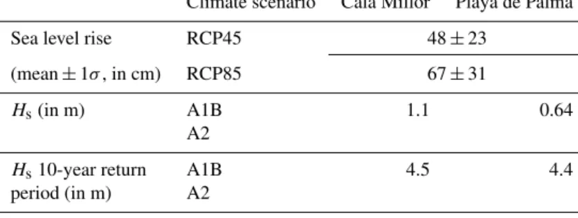
(5) A. R. Enríquez et al.: Changes in beach shoreline under climate change scenarios. 1079. Table 1. Input condition of the model set-up under climate change scenarios for the two beaches. See the text for details on their computation. Climate scenario. 2.5. Cala Millor. Playa de Palma. Sea level rise. RCP45. 48 ± 23. (mean ± 1σ , in cm). RCP85. 67 ± 31. Hs (in m). A1B A2. 1.1. 0.64. Hs 10-year return period (in m). A1B A2. 4.5. 4.4. Forcing of numerical models. The SWAN–SWASH model set-up described in Sect. 2.4 has been run under present-day and future climate conditions in both domains. The first step aims at validating the model performance, for which the present-day runs, forced with realistic offshore waves, have been compared against measured nearshore wave parameters. In the present-day runs deep water conditions were retrieved from the SIMAR database (Pilar et al., 2008), which is a 58-year wave reanalysis generated with the WAM model (WAMDI GROUP, 1988). The reanalysis, which is freely distributed by Puertos del Estado, covers the western Mediterranean and provides 3-hourly wave data up to 2011 and hourly data since then. The two closest SIMAR grid points to each of the domains were selected to force the SWAN model for the periods of validation (as detailed later). Although this data set has already been evaluated against observations (Pilar et al., 2008; MartínezAsensio et al., 2013, 2015), we have further compared the output with the offshore waves observed at Capdepera buoy in order to ensure the reliability of the forcing in the particular periods and locations studied here (Sect. 3.1). The sea level rise is included simply by indicating the still water level corresponding to the sea level in the projections by 2100. Once validated, the model set-up has been forced under future climate conditions. To so do, projected sea level rise together with changes in the wave climate have been run. A summary of the values used for sea level and waves is presented in Table 1. Regarding sea level, projections by 2100 have been estimated following Slangen et al. (2014), who provided the regional distribution of the different contributors to sea level change under two climate change scenarios, namely representative concentration pathway (RCP)45 and RCP85 (Moss et al., 2010). These are representative of moderate and large emission scenarios, respectively. Slangen et al. (2014) used an ensemble of 21 atmosphere–ocean coupled general circulation models (AOGCMs) from the Coupled Model Intercomparison Project Phase 5 (CMIP5) archive to estimate changes in ocean circulation and heat uptake contribution, atmospheric loading, land ice contribution (including all glaciers, ice caps and ice sheets on Greenland and www.nat-hazards-earth-syst-sci.net/17/1075/2017/. Antarctica), groundwater depletion and mass load redistribution worldwide, together with the associated uncertainties for each term. As the regional distribution of each component was provided, we selected the Mediterranean region and averaged the sum of the components as the input for projected sea level rise. The results lead to a regional sea level rise of 48 ± 23 cm and 67 ± 31 cm by 2100 for RCP45 and RCP85, respectively. Uncertainties quoted correspond to 1σ deviation from the ensemble mean (Slangen et al., 2014). Such values are thus consistent with the widely adopted values of sea level rise and the definition of the future climate scenarios (Brunel and Sabatier, 2009; Tamisea and Mitrovica, 2011; Church et al., 2011; IPCC, 2013) Changes in the wave climate during the 21st century have been obtained from regional wave projections over the western Mediterranean (Puertos del Estado et al., 2016). These projections were carried out using the WAM model with a spatial resolution of 1/6◦ (over the same grid as the SIMAR database) and forced with a set of dynamically-downscaled surface wind fields from AOGCMs. A total of six simulations were used, five corresponding to the A1B scenario and one to the A2 scenarios (IPCC SRES, 2000). Each projection was accompanied by a control simulation representing the climate of the last four decades of the 20th century, as it is usual practice. As the regional wave projections were computed before the adoption of the new set of RCP scenarios, for the purposes of the work, it is assumed here that the A1B (A2) scenario is equivalent to RCP45 (RCP85). One of these simulations is exemplarily represented in Fig. 5, in which the evolution of Hs under the A2 scenario is depicted for the mean regimen (Fig. 5a) and for the extremes (Fig. 5b). Changes in the mean and extreme wave regimes have been assessed by computing the differences between the values averaged over the period 2080–2100 (from the future projections, in blue in Fig. 5) and those averaged over 1980–2000 (from the control simulations, in black in Fig. 5). These differences reach 0.2 m under calm conditions and up to 0.3 during an extreme event. The obtained differences were then added to the hindcasted values from the reanalysis, which represent the best approach to the actual present-day climate (in red in Fig. 5). For each beach, the closest grid points (the same location as for the SIMAR database) were selected to simulate the future wave Nat. Hazards Earth Syst. Sci., 17, 1075–1089, 2017.

(6) 1080. A. R. Enríquez et al.: Changes in beach shoreline under climate change scenarios. Figure 5. Return periods in the A2 scenario for future projections (blue dashed line), control simulation (black dotted line) and hindcast (red line). Note that there are different time periods for the series as well as the overlapping of hindcast and control scenarios. The red line indicates the 1st day of hindcast time series.. Figure 6. Capdepera buoy observations (blue) and hindcasted SIMAR (black) time series of Hs , Tp and wave direction. RMSE and correlation are quoted for the wave direction (the values for Hs and Tp are quoted in Fig. 6).. climate. At the point representative of the deep water wave regime of Cala Millor, the resulting values for mean Hs were 1.20 and 0.95 m for the A2 and A1B scenarios, respectively, while in Playa de Palma the values were 0.63 m and 0.65, respectively. The storm events have been assessed computing the 10-year return periods by fitting a generalized Pareto distribution to each time series. The values obtained were 4.5 and 4.2 m under the A2 and A1B climate change scenarios in Cala Millor and 4.3 and 4.4 m in Playa de Palma. Given the similarities between the two wave climate change scenarios, a single (average) value for the simulations has been used (see Table 1). Regarding the wave direction, the changes are negligible and remain unchanged in the future simulations. In summary, six wave simulations have been carried out for each site to predict the shoreline changes under mean conditions: one for each of the two sea level rise scenarios Nat. Hazards Earth Syst. Sci., 17, 1075–1089, 2017. (RCP45 and RCP85) and one for their respective upper and lower uncertainty limits (i.e. plus 1σ and minus 1σ ). Please note that, for the sake of simplicity, hereinafter we will refer to ±1σ as our upper and lower uncertainty limits, respectively. In addition, four simulations have been performed for extreme conditions; due to computational constraints, we focused on the two highest sea levels for each scenario, that is, the occurrence of the 10-year return level storm occurring over the two sea level scenarios and their upper limit (i.e. for the mean value and the mean value +1σ ).. www.nat-hazards-earth-syst-sci.net/17/1075/2017/.

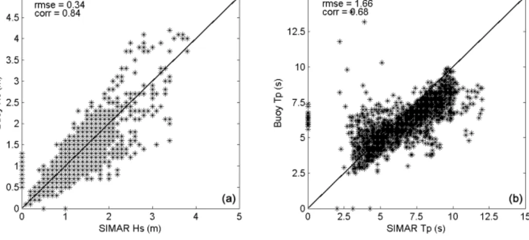
(7) A. R. Enríquez et al.: Changes in beach shoreline under climate change scenarios. 1081. Figure 7. Scatter plots of buoy observations vs. SIMAR hindcast for Hs (a) and Tp (b). RMSE and correlation are quoted in each figure.. 3. 3.1. Evaluation of model set-up under present-day climate conditions Comparison with wave observations. As described above, the SIMAR wave reanalysis has been taken as representative of the offshore wave conditions and used to force the numerical model set-up. To illustrate its reliability, the time series at the closest grid point in Cala Millor has been compared against observations from the nearby Capdepera buoy. The time series and scatter plots of the measured and modelled statistical wave parameters (Hs , Tp , θ ) are shown in Figs. 6 and 7 for a 3-month period (January– March 2014). The root mean square error (RMSE) and the correlation coefficient (ρ) between observed and modelled parameters are quoted in the figures. Results show that the hindcast agrees well with the observed Hs and Tp with correlations over 0.8 and a small RMSE. For wave direction, however, the correlation decreases down to 0.5, mostly due to the fact that the WAM resolution cannot properly resolve the coastal topography near the SIMAR location. A closer look at Fig. 6 (bottom panel) reveals that SIMAR contains waves from the NW (315◦ ) which are not recorded by the buoy. However, waves from the dominant directions (i.e. from N, 0◦ , to SE, 135◦ ) are not affected, and, therefore, Hs and Tp have enough accuracy to represent the wave climate of this offshore area. Despite the differences found in the wave direction, the advantages of using reanalysed data instead of observations for the input wave in SWAN are evident: first, the modelled time series are complete, while observations are often gappy; and second, the deep water waves can be propagated over large domains, thus providing values close to our two areas of study. Although the validation of the numerical hindcast is limited to a single grid point close to Cala Millor, previous assessments (e.g. Martínez-Asensio et al., 2013) also validated this hindcast, and it is therefore assumed that the reanalysis is equally valid for Playa de Palma. www.nat-hazards-earth-syst-sci.net/17/1075/2017/. The output of the SWAN model has been validated against observations in the two beaches. In Cala Millor the results of SWAN forced with SIMAR data were compared with nearshore wave observations during the period from 14 March to 14 April 2014 (i.e. a total of 755 h of simulation). The closest grid points of the SWAN model to each of the three directional wave ADCPs were selected. Resulting correlations, RMSEs and biases are listed in Table 2 for the three ADCPs and for the three wave parameters. Overall, the statistical parameters show good agreement between measurements and the model output, with correlations over 0.9 for Hs and Tp and over 0.7 for the wave direction. To further illustrate the model performance, observed and modelled time series are plotted in Figs. 8 and 9. Both reflect the ability of the model to capture the magnitude and variability of nearshore waves. Nevertheless, during the storm events recorded (as in 28 March), the model underestimates the observed Hs by up to 30 cm. In Playa de Palma, the simulated waves have been compared with the observations from a buoy moored at 23 m depth and with an ADCP at 17 m depth for the period from 1 to 30 September 2015 (i.e. a total of 720 h of simulation). The results are summarized in Table 3 and the time series are plotted in Figs. 10 and 11. Like in Cala Millor, there is a good agreement in Hs with correlations over 0.9. For Tp , however, observations display higher variability than modelled data, which makes the correlations drop to 0.32–0.34 and the bias reach 0.4–0.6 s for the buoy ADCP, respectively (see Fig. 11). Possible reasons for this discrepancy are the instrumental noise in measurements and/or the influence of local wind within the SWAN domain. The differences between observed and modelled wave directions are also larger than in Cala Millor, with non-significant correlations. The reason for the discrepancies in wave direction is probably the inability of the model to accurately represent the wave diffraction occurring at the SE of the bay of the Playa de Palma, where the buoy and the ADCP are located. This area is protected by. Nat. Hazards Earth Syst. Sci., 17, 1075–1089, 2017.

(8) 1082. A. R. Enríquez et al.: Changes in beach shoreline under climate change scenarios. Table 2. Comparison between SWAN results and nearshore wave observations in the Cala Millor beach. The period spanned by the series is from 14 March to 14 April 2014. ADCP 8 m. ADCP 12 m. ADCP 25 m. RMSE. Bias. Corr.. RMSE. Bias. Corr.. RMSE. Bias. Corr.. 0.13 1.21 25.60. 0.01 0.02 6.30. 0.97 0.94 0.74. 0.18 1.24 29.20. 0.03 0.01 3.65. 0.95 0.94 0.80. 0.23 1.22 40.43. 0.11 −0.22 14.20. 0.95 0.93 0.72. Hs (m) Tp (s) θp (◦ ). Figure 8. Hs , Tp and wave direction as modelled by SWAN and observed at the ADCP deployed at 12 m depth in the Cala Millor beach.. Table 4. Dates and forcing conditions of the SWASH simulations and results of the validation against observed shoreline position in the Cala Millor beach.. 27 March 28 March 1 April 2 April. Figure 9. SWAN vs. ADCP scatter plots of Hs (a) and Tp (b) in Cala Millor.. Table 3. Comparison between SWAN results and nearshore wave observations in Playa de Palma. The period spanned by the series is from 1 to 30 September 2015. Buoy 23 m. Hs (m) Tp (s) θp (◦ ). Hs (m). Tp (s). θ p (◦ ). RMSE (m). Bias (m). 1.6 0.8 0.5 1.1. 8.3 7.9 5.5 5.7. 13 28 137 134. 5.7 2.7 6.5 5.4. 3.2 −0.6 −3.2 −3.2. Table 5. Dates and forcing conditions of the SWASH simulations and results of the validation against observed shoreline position in Playa de Palma.. 3 September 15 September 28 September. Hs (m). Tp (s). θp (◦ ). RMSE (m). Bias (s). 0.4 0.6 0.4. 3.7 6.7 2.7. 154 223 47. 6.1 5.9 5.8. 1.5 1.7 1.4. a headland (see Fig. 4) that may cause worse results in wave direction.. ADCP 17 m. RMSE. Bias. Corr.. RMSE. Bias. Corr.. 0.19 1.56 46.19. 0.12 0.40 18.5. 0.95 0.32 0.29. 0.17 1.74 49.4. 0.09 0.60 30.9. 0.95 0.34 NS. Nat. Hazards Earth Syst. Sci., 17, 1075–1089, 2017. 3.2. Comparison with observed shoreline position. A total of four and three simulations have been carried out with the SWASH model for the Cala Millor and Playa de Palma beaches, respectively, in order to validate the model results with measurements of shoreline positions. The dates www.nat-hazards-earth-syst-sci.net/17/1075/2017/.

(9) A. R. Enríquez et al.: Changes in beach shoreline under climate change scenarios. 1083. Figure 10. Hs , Tp and wave direction as modelled by the SWAN model and observed at the buoy deployed at 23 m depth in Playa de Palma.. Figure 11. SWAN vs. ADCP scatter plots of Hs (a) and Tp (b) in Playa de Palma.. chosen for the validation correspond to dates in which the video monitoring provided good quality images, with them being also close to the dates when the bathymetry surveys were performed (they are listed in Tables 4 and 5). Wave makers were defined at the eastern boundary of the SWASH model domain in Cala Millor and at the southwestern boundary in Playa de Palma, in both cases with the SWAN wave conditions. These input wave conditions for the validation process are specified in Tables 4 and 5 for the indicated dates. Observed and modelled shoreline changes for each case study have been compared in Figs. 12 and 13 along the two beaches. Results show that the modelled shorelines line up with observations in all cases. In Cala Millor the agreement is better in the central part of the beach, while some differences are found in the northern and southernmost sector. It is important to remark that images obtained from the beach cameras are increasingly uncertain with the distance from the cameras (Sect. 2.3 for details). Therefore, part of the difference between the measured and simulated shoreline at the ends may come from this error in measurements. In Playa de Palma only the area between 39.51 and 39.53◦ N is used for the comparison as this is the stretch of the shoreline where the video system has the requested quality. We will also restrict the discussion on future projections to this sector.. www.nat-hazards-earth-syst-sci.net/17/1075/2017/. Figure 12. Observed (black) and modelled by SWASH (red) shoreline positions in Cala Millor.. The RMSEs and biases between observations and model results have been calculated for each case and are listed in Tables 4 and 5. These statistics must be set in a proper context in order to evaluate how good the model performance is. To do so, the temporal variability of the shoreline position has been estimated as the standard deviation (cross-shore) at each alongshore position for which 10 coastlines measured from video monitoring have been used. In Cala Millor, higher variability is observed, calculated between April and May 2014, in the central part of the beach (mean value of 8.4 m) and lower towards the ends, with a mean value along the entire beach of 5.5 m. Figure 14 shows the shorelines simulated for the case studies (red lines), the corresponding measured shorelines (blue lines) and the variability of the shoreline (grey area), zoomed in around an area at the centre of the beach. In the case of Playa de Palma, the shoreline displays a cross-shore variability of 6 m in the area around the centre of the beach and lower at the extremes, with a mean value of Nat. Hazards Earth Syst. Sci., 17, 1075–1089, 2017.

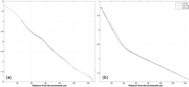
(10) 1084. A. R. Enríquez et al.: Changes in beach shoreline under climate change scenarios. Figure 15. Modelled (red) and observed (blue) shorelines positions in Playa de Palma with mean shoreline position (black line), its standard deviation (grey shadow) and the resolution of the pixels of the cameras (orange shadow). Figure 13. Observed (black) and modelled by SWASH (red) shoreline positions in Playa de Palma.. Figure 14. Modelled (red) and observed (blue) shorelines positions in Cala Millor with mean shoreline position (black line) and its standard deviation (grey shadow) zoomed in to the central sector.. 3 m, as calculated with observations between August and October 2014. The results are plotted in Fig. 15 in which again the central area has been zoomed in, in order to highlight the differences. Notably, the modelled shorelines are very similar to each other, because the forcing is also similar in the three case studies. 4. Shoreline changes under climate change scenarios. Since the model performance for present-day climate conditions is considered to be satisfactory, the same model setup has been used to assess the response of the shoreline under future climate change scenarios. Shoreline changes were simulated for both mean conditions and extreme waves (the latter being defined here as Hs corresponding to the 10-year return level) for the RCP45 and RCP85 climate change scenarios.. Nat. Hazards Earth Syst. Sci., 17, 1075–1089, 2017. Future projected changes in shoreline have been evaluated assuming that the present-day beach profile remains constant. In order to check the limitations of this assumption, we have run a numerical one-dimensional model capable of estimating profile changes under different mean sea level conditions. The model used here is PETRA (González et al., 2007), and it has been run for the central profile of each beach under the conditions of no sea level rise and 0.5 and 0.9 m of sea level rise and wave mean regime. The results of the model are plotted in Fig. 16 for both beaches, zoomed in to the nearshore sector where the largest changes are expected. Profile changes are, at most, 20 cm under the highest sea level rise of 0.9 m; that is, in these environments profile changes due to sea level rise are of the order of sandbar formation and mostly eroding the berm. We therefore have considered the variations in the beach profile to be negligible and the assumption of constant beach profile to be reasonable in this context. A second assumption in our climate change simulations is that the beach shape remains unchanged under future conditions. This means that we consider a constant direction in the mean wave energy flux. Thus, any redistribution in the alongshore sediments is neglected in front of the hydrodynamic response to increased mean sea level. The present-day modelled coastline has been used as a reference to assess the changes under climate change scenarios. The loss of aerial beach, defined here as the landward migration averaged over the entire beach, is indicated in Tables 6 and 7 for each simulation and for the mean and extreme conditions expected under climate change scenarios. For the extreme conditions, the maximum loss is also listed. In addition, Figs. 17 and 18 illustrate the maximum change in the shoreline position obtained for Cala Millor and Playa de Palma (corresponding to extreme wave conditions under the RCP85 +1σ scenario). Major changes are projected to occur in the central part of the Cala Millor beach, where the higher variability is shown (see www.nat-hazards-earth-syst-sci.net/17/1075/2017/.

(11) A. R. Enríquez et al.: Changes in beach shoreline under climate change scenarios. 1085. Figure 16. Changes in the cross profile in Cala Millor (a) and Playa de Palma (b) in the nearshore area under different sea levels. Table 6. Loss of aerial beach (defined here as the landward migration of the shoreline averaged over the entire beach) for both the mean and extreme conditions expected under climate change scenarios in Cala Millor (in m). For the extreme conditions, the maximum loss is also quoted. Sea level rise. Mean conditions. (climate scenario ± uncertainty, in cm) 0.25 (RCP45 −1σ ) 0.36 (RCP85 −1σ ) 0.48 (RCP45) 0.67 (RCP85) 0.71 (RCP45 +1σ ) 0.98 (RCP85 +1σ ). Figure 17. Present-day shoreline position (in black) and landward migration (in red) in the worst case scenario (mean sea level rise under RCP85 and extreme wave conditions) by the end of the 21st century in the Cala Millor beach.. www.nat-hazards-earth-syst-sci.net/17/1075/2017/. Extreme conditions. Mean loss (m). Mean loss (m). Max loss (m). 7.2 10.7 11.7 17.5 17.5 24.2. – – 18.5 21.8 24.6 29.0. – – 29.4 38.0 39.5 49.3. Figure 18. Present-day shoreline position (in black) and landward migration (in red) in the worst case scenario (mean sea level rise under RCP85 and extreme wave conditions) by the end of the 21st century in Playa de Palma.. Nat. Hazards Earth Syst. Sci., 17, 1075–1089, 2017.

(12) 1086. A. R. Enríquez et al.: Changes in beach shoreline under climate change scenarios. Table 7. Loss of aerial beach (defined here as the landward migration of the shoreline averaged over the entire beach) for both the mean and extreme conditions expected under climate change scenarios in Playa de Palma (in m). For the extreme conditions, the maximum loss is also quoted. Sea level rise. Mean conditions. (climate scenario ± uncertainty, in cm) 0.25 (RCP45 −1σ ) 0.36 (RCP85 −1σ ) 0.48 (RCP45) 0.67 (RCP85) 0.71 (RCP45 +1σ ) 0.98 (RCP85 +1σ ). Fig. 14). Larger relative impacts (loss of width), however, are projected towards the extremes of the beach, as these are the narrower sectors. In Playa de Palma, the projected changes in the shoreline are quite uniform along the beach. Since projected changes in Hs by 2100 are small, their potentially hazardous effects depend primarily on the mean sea level with which they are combined. In Cala Millor, the averaged coastline retreat ranges between 7 m under the moderate low scenarios and 24 m with the highest sea level rise considered. During extreme wave conditions the shoreline would retreat up to 29 m on average and may reach 49 m at some parts of the beach. With such values the flooding would reach the urbanized area over the promenade. However, it must be pointed out that the topography does not include the height of the wall backing the beach and the simulations were stopped there, so the flooding extension could actually be underestimated. In Playa de Palma the average coastline retreat ranges from the 7 m obtained for the low scenario to the 21 m obtained for the upper limit considered here. Under extreme conditions, the loss of the beach in Playa de Palma increases with higher sea level rise, and, in all the cases investigated, the water level reaches the promenade at least in part of the domain (Table 6). 5. Summary and conclusions. This paper has investigated the capabilities of state-of-theart numerical models to reproduce the changes in the shoreline position in the Cala Millor and Playa de Palma beaches. These two case studies were selected for two main reasons. First, they are representative of many other anthropized beaches in the Balearic Islands (and of many other beaches of the Mediterranean Sea): they are beaches located in urbanized areas, backed by walls, and therefore with limited possible landward migration of the shoreline. Second, these two sites are part of the beach monitoring programme carried out by SOCIB, and, consequently, a wide and complete set of observations is available, allowing the validation of the numerical models against measurements. Furthermore, the two beaches are exposed to offshore wave conditions from difNat. Hazards Earth Syst. Sci., 17, 1075–1089, 2017. Extreme conditions. Mean loss (m). Mean loss (m). Max loss (m). 7 8.2 11.3 14.8 15.7 21.4. – – 17 20.5 23.4 27.9. – – 30 30 30 30. ferent directions and different wave heights, with Playa de Palma being located inside a bay and Cala Millor facing the open sea. Much effort has been devoted to the validation of the model set-up to ensure that the chosen combination of SWAN–SWASH models is able to reproduce the shoreline variability within a reasonable accuracy. In both cases, modelled and observed Hs from nearshore instruments were in very good agreement, with correlations over 0.9. This increases our confidence in the forcing of the SWASH model. In turn, a satisfactory correspondence between the observed and modelled shoreline position has been found. The agreement between modelled and observed shorelines was better in the central sector of the beaches. This is because the observations derived from the video monitoring system are more reliable close to the location of the cameras and also because the SWASH model configuration requires a smooth bathymetry which can misrepresent some parts of the shore, as is the case for the southernmost sector of Cala Millor where a rock bed and a small cliff distort the wave field. Regarding the projections of the shoreline changes under climate scenarios of sea level and wave climate, a major assumption of our study is that the morphology of the beach will not change in the future. That is, both the beach shape and the profile will be the same under the climate conditions at the end of the century. It is well known that beach profile evolves in response to storms, moderate wave conditions and sea level rise causing changes in the beach morphology (e.g. erosion followed by recovery episodes, see Short, 1996; Simeone et al., 2014; Smallegan et al., 2016; Davidson-Arnott et al., 2002). It has also been demonstrated that the changes in the beach profile play a smaller role in the shoreline retreat due to sea level rise and waves. On top of the above reasons, numerical approaches reproducing the long-term morphological response of the beach are still very limited (e.g. Ranasinghe et al., 2012). Under the assumptions outlined above, we have found that the retreat in the future shoreline at both sites, Cala Millor and Playa de Palma, are primarily a consequence of waves acting onto a higher mean sea level. It must be mentioned. www.nat-hazards-earth-syst-sci.net/17/1075/2017/.

(13) A. R. Enríquez et al.: Changes in beach shoreline under climate change scenarios that changes in the wave climate are small and the impact of extreme waves increases mostly because they are projected to occur concurrently with higher sea levels. The results indicate that the beach regression varies between 7 and 24 m along Cala Millor and between 7 and 21 m in Playa de Palma, depending on the climate change scenario considered. This loss is further exacerbated under moderate (return period of 10 years) storm conditions, which may induce a temporary flooding reaching over 49 m in Cala Millor and 30 m in Playa de Palma, thus likely overtopping the walls of the promenade. The Playa de Palma coastal retreat is lower than in Cala Millor due to the steeper slope of the beach profile. As pointed out above in the introduction, the approach proposed here does not consider beach erosion, which means that the above estimates are conservative and could be biased low if erosion acts by removing beach sediments and accelerating aerial beach loss (Brunel and Sabatier, 2009). Playa de Palma and Cala Millor, like many other typical urban Mediterranean beaches, are subject to high touristic pressure, especially during the summer season, and thus concentrate valuable assets and infrastructures. Since tourism constitutes the main economic activity of a large fraction of the region, the social, environmental and economic impacts of future sea level rise are anticipated if no adaptation measures are implemented.. Data availability. The data used to validate the methodology (observations from shorelines and buoys) are freely available through the SOCIB data repository. The bathymetries are provided by SOCIB upon request. The results of the present study will also be provided upon request to the corresponding author.. Competing interests. The authors declare that they have no conflict of interest.. Acknowledgements. This work is supported by the CLIMPACT (CGL2014-54246-C2-1-R) funded by the Spanish Ministry of Economy) and MORFINTRA (CTM2015-66225-C2-2-P). Alejandra R. Enríquez acknowledges an FPI grant associated with the CLIMPACT project. Marta Marcos acknowledges a “Ramón y Cajal” contract funded by the Spanish Government. We thank Puertos del Estado for providing deep water wave data from the SIMAR database. Topo-bathymetries and video-monitoring observations are part of the beach monitoring facility of SOCIB. The authors are grateful to Aimée Slangen for providing the data for the regional sea level rise scenarios. Edited by: Paolo Tarolli Reviewed by: three anonymous referees. www.nat-hazards-earth-syst-sci.net/17/1075/2017/. 1087. References Booij, N., Ris, R. C., and Holthuijsen, L. H.: A thirdgeneration wave model for coastal regions 1. Model description and validation, J. Geophys. Res.-Oceans, 104, 7649–7666, https://doi.org/10.1029/98JC02622, 1999. Brunel, C. and Sabatier, F.: Potential influence of sealevel rise in controlling shoreline position on the French Mediterranean Coast, Geomorphology, 107, 47–57, https://doi.org/10.1016/j.geomorph.2007.05.024, 2009. Cazenave, A. and Le Cozannet, G.: Sea level rise and its coastal impacts, Earth’s Future, 2, 15–34, https://doi.org/10.1002/2013EF000188, 2014. Church, J. A., Gregory, J. M., White, N. J., Platten, S. M., and Mitrovica, J. X.: Understanding and projecting sea level change, Oceangraphy, 24, 130–143, https://doi.org/10.5670/oceanog.2011.33, 2011. Church, J. A., Clark, P. U., Cazenave, A., Gregory, J. M., Jevrejeva, S., Levermann, A., Merrifield, M. A., Milne G. A., Nerem, R. S., Nunn, P. D., Payne, A. J., Pfeffer, W. T., Stammer, D., and Unnikrishnan, A. S.: Sea Level Change, in: Climate Change 2013: The Physical Science Basis. Contribution of Working Group I to the Fifth Assessment Report of the Intergovernmental Panel on Climate Change, edited by: Stocker, T. F., Qin, D., Plattner, G.K., Tignor, M., Allen, S. K., Boschung, J., Nauels, A., Xia, Y., Bex, V., and Midgley, P. M., Cambridge University Press, Cambridge, United Kingdom and New York, NY, USA, 2013. Davidson-Arnott, R. G. D., van Proosdij, D., Ollerhead, J., and Schostak, L.: Hydrodynamics and sedimentation in salt marshes: examples from a macrotidal marsh, Bay of Fundy, Geomorphology, 48, 209–231, https://doi.org/10.1016/S0169555X(02)00182-4, 2002. Eurostat: The Mediterranean and Black Sea basins, available at: http://ec.europa.eu/eurostat/en/web/products-statistics-in-focus/ -/KS-SF-11-014 last access: 23 March 2011. Feagin, R. A., Sherman, D. J., and Grant, W. E.: Coastal erosion, global sea-level rise, and the loss of sand dune plant habitats, Front. Ecol. Environ., 3, 359–364, 2005. FitzGerald, D. M., Fenster, M. S., Argow, B. A., and Buynevich, I. V.: Coastal impacts due to sealevel rise, Annu. Rev. Earth Pl. Sc., 36, 601–647, https://doi.org/10.1146/annurev.earth.35.031306.140139, 2008. González, M., Medina, R., Gonzalez-Ondina, J., Osorio, A., Méndez, F. J., and García, E.: An integrated coastal modeling system for analyzing beach processes and beach restoration projects, SMC, Comput. Geosci., 33, 916–931, https://doi.org/10.1016/j.cageo.2006.12.005, 2007. Guimarães, P. V., Farinha, L., Toldo Jr., E., Diaz-Hernandez, G., and Akhmatskaya, E.: Numerical simulation of extreme wave runup during storm events in Tramandí Beach, Rio Grande do Sul, Brazil, Coast. Eng., 95, 171–180, https://doi.org/10.1016/j.coastaleng.2014.10.008, 2015. Gutierrez, B. T., Nathaniel, P. G., and Thieler, R. E.: A Bayesian network to predict coastal vulnerability to sea level rise, J. Geophys. Res., 116, F02009, https://doi.org/10.1029/2010JF001891, 2011. Hanson, S., Nicholls, R., Ranger, N., Halleegatte, S., CorfeeMorlot, J., Herweijer, C., and Chateau, J.: A global ranking of port cities with exposure to climate extremes, Climate Change, 104, 89–111, https://doi.org/10.1007/s10584-010-9977-4, 2011.. Nat. Hazards Earth Syst. Sci., 17, 1075–1089, 2017.

(14) 1088. A. R. Enríquez et al.: Changes in beach shoreline under climate change scenarios. IPCC: Climate Change 2013: The Physical Science Basis, Contribution of Working Group I to the Fifth Assessment Report of the Intergovernmental Panel on Climate Change, edited by: Stocker, T. F., Qin, D., Plattner, G.-K., Tignor, M., Allen, S. K., Boschung, J., Nauels, A., Xia, Y., Bex, V., and Midgley, P. M., Cambridge University Press, Cambridge, United Kingdom and New York, NY, USA, 1535 pp., https://doi.org/10.1017/CBO9781107415324, 2013. IPCC SRES: Intergovernmental Panel on Climate Change: Special Report on Emissions Scenarios, edited by: Nakicenovic, N. and Swart, R., Cambridge Univ. Press, New York, 612 pp., 2000. Le Cozannet, G., Garcin, M., Yates, M., Idier, D., and Meyssignac, B.: Approaches to evaluate the recent impacts of sealevel rise on shoreline changes, Earth-Sci. Rev., 13, 47–60, https://doi.org/10.1016/j.earscirev.2014.08.005, 2014. Martínez-Asensio, A., Marcos, M., Jordà, G., and Gomis, D.: Calibration of a new wind-wave hindcast in the Western Mediterranean, J. Marine Syst., 121–122, 1–10, https://doi.org/10.1016/j.jmarsys.2013.04.006, 2013. Martínez-Asensio, A., Tsimplis, M. N., Marcos, M., Feng, X., Gomis, D., Jordà, G., and Josey, S. A.: Response of the North Atlantic wave climate to atmospheric modes of variability, Int. J. Climatol., 36, 1210–1225, https://doi.org/10.1002/joc.4415, 2015. Medellín, G., Brinkkemper, J. A., Torres-Freyermuth, A., Appendini, C. M., Mendoza, E. T., and Salles, P.: Run-up parameterization and beach vulnerability assessment on a barrier island: a downscaling approach, Nat. Hazards Earth Syst. Sci., 16, 167– 180, https://doi.org/10.5194/nhess-16-167-2016, 2016. Morales-Márquez, V., Orfila, A., Gómez-Pujol, L. L., Conti, D., Simarro, G., Álvarez-Ellacuría, A., Osorio, A. F., Marcos, M., and Galán, A.: Numerical and observational data for addressing the beach dynamics and recovery associated to a storm group impact, Mar. Geol., in review, 2017. Moss, R. H., Edmonds, J. A., Hibbard, K. A., Manning, M. R., Rose, S. K., Van Vuuren, D. P., Carter, T. R., Emori, S., Kainuma, M., Kram, T., Meehl, G. A., Mitchell, J. F. B., Nakicenovic, N., Riahi, K., Smith, S. J., Stouffer, R. J., Thomson, A. M., Weyant, J. P., and Wilbanks, T. J.: The next generation of scenarios for climate change research and assessment, Nature, 463, 747–756, https://doi.org/10.1038/nature08823, 2010. Nicholls, R. and Cazenave, A.: Sea-Level Rise and Its Impact on Coastal Zones, Science, 328, 1517–1520, https://doi.org/10.1126/science.1185782, 2010. Nieto, M. A., Garau, B., Balle, S., Simarro, G., Zarruk, G. A., Ortiz, A., Tintoré, J., Álvarez-Ellacuría, A., Gómez-Pujol, L., and Orfila, A.: SIRENA: An open source, low cost video-based coastal zone monitoring system, Earth Surf. Proc. Land., 35, 1712–1719, https://doi.org/10.1002/esp.2025, 2010. Passeri, D. L., Hagen, S. C., Medeiros, S. C., Bilskie, M. V., Alizad, K., and Wang, D.: The dynamic effects of sea level rise on lowgradient coastal landscapes: A review, Earth’s Future, 3, 159– 181, https://doi.org/10.1002/2015EF000298, 2015. Pilar, P., Guedes Soares, C., and Carretero, J. C.: 44-year wave hindcast for the NortEast Atlantic European coast, Coast. Eng., 55, 861–871, https://doi.org/10.1016/j.coastaleng.2008.02.027, 2008.. Nat. Hazards Earth Syst. Sci., 17, 1075–1089, 2017. Poulter, B. and Halpin, P. N.: Raster modelling of coastal flooding from sea-level rise, Int. J. Geogr. Inf. Sci., 22, 167–182, https://doi.org/10.1080/13658810701371858, 2008. Plant, N. G., Thieler, E. R., and Passeri, D. L.: Coupling centennialscale shoreline change to sea-level rise and coastal morphology in the Gulf of Mexico using a Bayesian network, Earth’s Future, 4, 143–158, https://doi.org/10.1002/2015EF000331, 2016. Puertos del Estado, Agenca Estatal de Meteorología (AEMET), and Instituto Mediterráneo de Estudios Avanzados (IMEDEA): Vulnerabilidad de los puertos españoles ante el cambio climático, Vol. 1, Tendencias de variables físicas oceánicas y atmosféricas durante las últimas décadas y proyecciones para el siglo XXI. Edi., Puertos del Estado, Madrid, 2016. Ranasinghe, R., Callaghan, D., and Stive, M. J. F.: Estimating coastal recession due to sea level rise: Beyond the Bruun rule, Climatic Change, 110, 561–574, https://doi.org/10.1007/s10584011-0107-8, 2012. Ruju, A., Lara, J. L., and Losada, I. J.: Numerical analysis of run-up oscillations under dissipative conditions, Coast. Eng., 86, 45–56, https://doi.org/10.1016/j.coastaleng.2014.01.010, 2014. Short, A. D.: The role of wave height, period, slope, tide range and embaymentisation in beach classifications: a review, Rev. Chil. Hist. Nat., 69, 589–604, 1996. Simarro, G., Ribas, F., Álvarez, A., Guillén, J., Chic, Ò., and Orfila, A.: ULISES: An open source code for extrinsic calibrations and planview generations in coastal video monitoring systems, J. Coastal Res., in press, 2017. Simeone, S., De Falco, G., Quattrochi, G., and Cucco, A.: Morphological changes of a Mediterranean beach over one year (San Giovanni Sinis, western Mediterranean), J. Coastal Res., 70, 217–222, 2014. Slangen, A. B. A., Carson, M., Katsman, C. A., van de Wal, R. S. W., Köhl, A., Vermeersen, L. L. A., and Stammer, D.: Projecting twenty-first century regional sea-level changes, Climate Change, 124, 317–332, https://doi.org/10.1007/s10584014-1080-9, 2014. Smallegan, S. M., Irish, J. L., Van Dongeren, A. R., and Den Bieman, J. P.: Morphological response of a sandy barrier island with a buried seawall during Hurricane Sandy, Coast. Eng., 110, 102– 110, 2016. Stive, M. J. F.: How important is global warming for coastal erosion?, Climatic Change, 64, 27–39, https://doi.org/10.1023/B:CLIM.0000024785.91858.1d, 2004. Tamisiea, M. E. and Mitrovica, J. X.: The moving boundaries of sea level change: Understanding the origin of geographic variability, Oceanography, 24, 24–39, https://doi.org/10.5670/oceanog.2011.25, 2011. Tintoré, J., Vizoso, G., Casas, B., Heslop, E., Pascual, A., Orfila, A., Ruiz, S., Martínez-Ledesma, M., Torner, M., Cusí, S., Dierdrich, A., Balaguer, P., Gómez-Pujol, L., Álvarez-Ellacuría, A., Gómara, S., Sebastian, K., Lora, S., Beltrán, J. P., Renault, L., Juzà, M., Álvarez, D., March, D., Garau, B., Castilla, C., Cañellas, T., Roque, D., Lizarán, I., Pitarch, S., Carrasco, M. A., Lana, A., Mason, E., Escudier, R., Conti, D., Sayol, J. M., Barceló, B., Alemany, F., Reglero, P., Massuti, E., Vélez-Belechí, P., Ruiz, J., Oguz, T., Gómez, M., and Manriquez, M.: SOCIB: The Balearic Islands coastal ocean observing and forecasting system responding to science, technology and society needs, Marine Soci-. www.nat-hazards-earth-syst-sci.net/17/1075/2017/.

(15) A. R. Enríquez et al.: Changes in beach shoreline under climate change scenarios ety Journal, 47, 101–117, https://doi.org/10.4031/MTSJ.47.1.10, 2013. Villatorio, N., Silva, R., Méndez, F. J., Zanuttigh, B., Pan, S., Trifonova, E., Losada, I. J., Izaguirre, C., Simmonds, D., Reeve, D. E., Mendoza, E., Martinelli, L., Formentin, S. M., Galiatsatou, P., and Eftimova, P.: An approach to assess flooding and erosion risk for open beaches in a changing climate, Coast. Eng., 87, 50–76, https://doi.org/10.1016/j.coastaleng.2013.11.009, 2014. WAMDI Group: The WAM model – a third generation ocean wave prediction model, J. Phys. Oceanogr., 18, 1775–810, https://doi.org/10.1175/15200485(1988)018<1775:TWMTGO>2.0.CO;2, 1988.. www.nat-hazards-earth-syst-sci.net/17/1075/2017/. 1089. Wu, S.-Y., Yarnal, B., and Fisher, A.: Vulnerability of coastal communities to sea-level rise: a case study of Cape May County, New Jersey, USA, Clim. Res., 22, 255–277, https://doi.org/10.3354/cr022255, 2002. Zijlema, M., Stelling, G., and Smit, P.: SWASH: An operational public domain code for simulating wave fields and rapidly varied flows in coastal waters, Coast. Eng., 58, 992–1012, https://doi.org/10.1016/j.coastaleng.2011.05.015, 2011. Zhang, K., Douglas, B. C., and Leatherman, S. P.: Global warming and coastal erosion, Climate Change, 64, 41–58, https://doi.org/10.1023/B:CLIM.0000024690.32682.48, 2004.. Nat. Hazards Earth Syst. Sci., 17, 1075–1089, 2017.

(16)