The evolution of risk perception in Chile : a comparison of cross sectional studies (2001 2013)

Texto completo

(1)PONTIFICIA UNIVERSIDAD CATÓLICA DE CHILE ESCUELA DE INGENIERÍA. THE EVOLUTION OF RISK PERCEPTION IN CHILE: A COMPARISON OF CROSS SECTIONAL STUDIES (2001-2013). CAMILA ANDREA ZACHARIAS MOLINA. Thesis submitted to the Office of Research and Graduate Studies in partial fulfillment of the requirements for the Degree of Master of Science in Engineering Advisor: LUIS ABDÓN CIFUENTES LIRA. Santiago de Chile, December, 2013  2013, Camila Andrea Zacharias Molina.

(2) PONTIFICIA UNIVERSIDAD CATÓLICA DE CHILE ESCUELA DE INGENIERÍA. THE EVOLUTION OF RISK PERCEPTION IN CHILE: A COMPARISON OF CROSS SECTIONAL STUDIES (2001-2013). CAMILA ANDREA ZACHARIAS MOLINA. Members of the Committee: LUIS ABDÓN CIFUENTES LIRA NICOLÁS MAJLUF SAPAG NICOLÁS BRONFMAN CÁCERES JUAN ENRIQUE COEYMANS. Thesis submitted to the Office of Research and Graduate Studies in partial fulfillment of the requirements for the Degree of Master of Science in Engineering. Santiago de Chile, December, 2013.

(3) I dedicate this work to my family and all those who helped me in this process. A special feeling of gratitude to my loving parents, Nora and Jaime, who have taught me everything and have always encouraged me to follow my dreams.. iii.

(4) ACKNOWLEDGEMENTS I would like to express my gratitude to my supervisor, Dr. Luis Cifuentes, who always supported me throughout my research with his patience and knowledge, whilst allowing me the room to work in my own way. I would also like to thank my co-advisor, Dr. Nicolás Bronfman, for his infinite patience and sharing with me long hours of reflection and reading. Throughout my thesis-writing period, they provided encouragement, sound advice, good teaching, good company, and lots of good ideas. I would have been lost without them. I especially want to thank them for opening the doors of their homes, sharing their infinite knowledge of risk analysis with me, and giving me their precious time. I would also like to thank my committee members, Dr. Nicolás Majluf and Dr. Juan Enrique Coeymans, for taking time from their busy schedules to be a part of this investigation. Above all, I would like to thank my family. I would not have contemplated this road if not for my parents, Jaime and Nora, who instilled within me a love for creativity, sciences and exploring the unknown. I am very grateful for their love and dedication, and the many years of unconditional support during my childhood, undergraduate years, and in my master’s degree. I would like to thank my sisters, Javiera, Constanza and Macarena, who always found a way to make me laugh, even during the most stressful periods of this process. No one understands my weirdness and humor like you do. This thesis would also not be possible without the love and unequivocal support of my boyfriend Mauricio, who has put up with me for the many months I have been welded to my computer, has been my emotional pillar at all times, and has shared every excitement and frustration with me throughout this process. I take this opportunity to thank my friends, Marianne and Francisca, who have been my partners through this journey. I thank them for all the laughs, conversations and their constant encouragement. They have supported me through the dark times, celebrated with me through the good, and have been brilliant and understanding when I needed them to be.. iv.

(5) Table of Contents. Acknowledgements ..........................................................................................................iv Resumen ...........................................................................................................................ix Abstract ............................................................................................................................. x 1. Introduction .............................................................................................................. 1. 2. Theoretical Framework ........................................................................................... 4. 3. 4. 2.1. Expert and laypeople judgments about risk .................................................. 4. 2.2. The Psychometric Paradigm ........................................................................... 5. 2.3. The availability heuristic and its relationship with natural hazards .......... 7. 2.4. Risk perception studies in Chile ..................................................................... 7. 2.5. Changes in Chile over the last decade ............................................................ 8. Methods and Data .................................................................................................. 11 3.1. Instrument design .......................................................................................... 11. 3.2. Instrument validation .................................................................................... 13. 3.3. Instrument Implementation .......................................................................... 14. 3.4. Data Analysis .................................................................................................. 16. 3.4.1. Tukey’s HSD Test ........................................................................................ 17. 3.4.2. Normal probability Q-Q plot........................................................................ 17. 3.4.3. Levene’s Test of Equality of Variances ....................................................... 18. 3.4.4. Principal Components Analysis ................................................................... 18. 3.4.5. OLS Regression Model ................................................................................ 19. 3.4.6. Independent Samples T-Test ........................................................................ 19. Results ..................................................................................................................... 20 4.1. Sample population.......................................................................................... 20. 4.2. Transformation of Likert scales ................................................................... 22. 4.3. Normality of the data ..................................................................................... 22 v.

(6) 4.4. Homogeneity of variance ............................................................................... 23. 4.5. Description of Attributes ............................................................................... 23. 4.6. Factor analysis ................................................................................................ 26. 4.6.1. Combined Factor Analysis ........................................................................... 27. 4.7. Changes in male and female perceptions during the last decade .............. 31. 4.8. Relationship between factors of the psychometric paradigm and. perceptions of analysis variables .............................................................................. 35. 5. 4.9. Changes in social perceptions analyzed by type of hazard ........................ 36. 4.10. Changes in social perceptions analyzed by hazard ..................................... 41. Conclusions ............................................................................................................. 48 5.1. A challenge for regulators ............................................................................. 48. 5.2. Perspectives for future investigations........................................................... 50. References ....................................................................................................................... 52 Annexes ........................................................................................................................... 60 Annex A: Normal Q-Q plots ..................................................................................... 61 Annex B: Independent samples T-test ..................................................................... 64 Annex C: Mean scores for risk attributes by hazard and year.............................. 71 Annex D: Mean values per hazard for risk, benefit and acceptability (2001-2013) ...................................................................................................................................... 73 Annex E: Questionnaires administered to the sample population (2013) ............. 79. vi.

(7) Index of Tables Table 3-1. Attributes and analysis variables included in each questionnaire .................. 12 Table 3-2. List of hazards evaluated ................................................................................ 13 Table 3-3: Sample obtained per questionnaire ................................................................. 16 Table 4-1. Description of Sample .................................................................................... 20 Table 4-2. Nuclear weapons and genetic engineering’s homogenous subsets for α = 0.05 (Tukey's HSD, dependent variable = social acceptability) .............................................. 21 Table 4-3. Mean values (standard deviations) for risk attributes in 2001 and 2013 ........ 24 Table 4-4. Correlation matrix of risk attributes (combined 2001-2013) .......................... 25 Table 4-5: Rotated components matrix for each year ...................................................... 26 Table 4-6. Rotated components matrix for factor analysis 2001-2013 ............................ 27 Table 4-7. Mean scores (standard deviations) for analysis variables in 2001 and 2013 .. 32 Table 4-8. Mean scores for analysis variables by gender and year .................................. 34 Table 4-9: Bivariate correlation between social risk, social benefit and social acceptance .......................................................................................................................................... 35 Table 4-10. Standarized coefficients from OLS regression models ................................ 36 Table 4-11. Risk perception mean scores by type of hazard............................................ 37 Table 4-12. Benefit perception mean scores by type of hazard ....................................... 38 Table 4-13. Acceptability perceptions mean scores by type of hazard ............................ 39 Table 7-1. Independent samples T-test for analysis variables (2001-2013) and Levene’s test for equality of variances ............................................................................................ 64 Table 7-2. Mean scores for risk attributes by hazard and year ........................................ 71 Table 7-3. Social risk scores by hazard and year ............................................................. 73 Table 7-4. Social benefit scores by hazard and year ........................................................ 75 Table 7-5. Social acceptability scores by hazard and year............................................... 77. vii.

(8) Index of Figures. Figure 4-1: Position of hazards in factorial map in 2001 and 2013 (movement shown by arrows).............................................................................................................................. 29 Figure 4-2. Changes in risk, benefit and acceptability perceptions between 2001 and 2013. ................................................................................................................................. 40 Figure 4-3. Changes in risk perception by hazard............................................................ 42 Figure 4-4. Changes in benefit perception by hazard ...................................................... 44 Figure 4-5. Changes in acceptability perception by hazard ............................................. 45 Figure 4-6. Risk-Benefit Map (movement from 2001 to 2013 perception scores shown by arrows)......................................................................................................................... 47 Figure 7-1. Normal Q-Q plots for social risk in 2001 ...................................................... 61 Figure 7-2. Normal Q-Q plots for social risk in 2013 ..................................................... 61 Figure 7-3. Normal Q-Q plots for social benefit in 2001................................................. 62 Figure 7-4. Normal Q-Q plots for social benefit in 2013................................................. 62 Figure 7-5. Normal Q-Q plots for social acceptability in 2001 ....................................... 63 Figure 7-6. Normal Q-Q plots for social acceptability in 2013 ....................................... 63. viii.

(9) RESUMEN. Chile ha experimentado muchos cambios sociales y culturales durante la última década. Con un aumento del PIB per cápita y alta estabilidad política, Chile se ha posicionado como uno de los países más desarrollados de la región. A la vez, grandes desastres naturales han afectado a la población. El más relevante ocurrió en el 2010, cuando un terremoto de magnitud 8.9 y un tsunami afectaron al 80% de la población chilena, algo que no había ocurrido a este nivel de magnitud desde 1960. Con todos estos cambios, es esperable que la percepción de riesgo de la población haya cambiado en la última década. El principal objetivo de esta investigación es evaluar el cambio en percepciones de riesgo en Chile entre el 2001 y el 2013. Para llevar esto a cabo, se midieron las percepciones de riesgo actuales y se contrastaron con aquellas evaluadas en el estudio de Bronfman y Cifuentes (2003). Basándose en el paradigma sicométrico, y utilizando una encuesta similar a la del estudio pasado, se estudiaron las diferencias de percepciones de riesgo, beneficio y aceptabilidad para 31 peligros distintos.. La encuesta fue. implementada en Santiago de Chile en junio del 2013, donde 1.273 personas participaron del estudio. Los resultados muestran que el paradigma sicométrico no muestra grandes diferencias en la última década. El factor 1 (“Riesgo Terrible”) se mantiene como el más importante a la hora de explicar las percepciones de la población para el 2001 y el 2013. Las percepciones de riesgo, beneficio y aceptabilidad muestran cambios significativos en la última década: la población actual percibe los peligros con mayor riesgo y menor aceptabilidad que hace una década, particularmente para desastres naturales, males sociales y peligros ambientales. Las implicancias de este estudio en políticas públicas son discutidas.. Palabras claves: percepción de riesgo, evolución de percepción de riesgo, paradigma sicométrico, diferencias entre géneros, estudio transversal. ix.

(10) ABSTRACT Chile has experienced several social and cultural changes during the last 15 years. Percapita income growth and political stability have placed Chile in a leading position in South America, and development has produced many changes in its society. The population has raised awareness towards environmental hazards and inequality issues in health and education. Natural disasters have also affected the population. In 2010 Chile suffered an 8.9 magnitude earthquake and tsunami, something not experienced by the Chilean population since 1960. With all these changes, it is expected that public risk perceptions are different than it was a decade ago. The main objective of this investigation is to assess the change in risk perception in Chile between 2001 and 2013. To achieve this, current public concerns and perceptions of risk were characterized and contrasted with those quantified and reported a decade ago by the study of Bronfman and Cifuentes (2003). Based on the psychometric paradigm, and using a similar survey to the one implemented before, differences in perceptions of risk, benefit and acceptability for 31 hazards were studied. The survey was implemented to 1,273 participants from Santiago in June 2013. Results show that the psychometric paradigm has no relevant differences over the last decade. Factor 1 (Dread Risk) remains as the most important factor in explaining risk perception for 2001 and 2013. Perceived risk, benefit and acceptability have significantly changed over the past decade: today’s population perceives hazards with higher risk and less acceptability than a decade ago, especially regarding natural disasters, social ills and environmental hazards. Men and women show significant differences between their perceptions of 2001 and 2013. Main implications for public policies are discussed.. Key words: Risk perception, evolution of risk perception, psychometric paradigm, gender differences, cross sectional study. x.

(11) 1. 1. INTRODUCTION. Public perceptions of risk are a focal point of discussions regarding the management of different hazards (technologies, activities, substances, etc.). The policies that should be adopted and the structure of policy-making processes are often determined by different views of what the public knows and wants. The problem about this is that, more often than not, these views are based on anecdotal observation or speculation (Fischhoff et al., 1982). In order to develop appropriate policies regarding acceptability levels of risk and risk communication strategies, among others, empirical evidence regarding what the public truly knows and wants is needed. The study of risk perceptions began in the 1970’s, with the initial investigations by (Starr, 1969), (Fischhoff et al., 1978) and (Slovic et al., 1980). Using questionnaires with psychometric scales, researchers asked the public directly what their perceptions of risk and benefit were, regarding several hazards. Numerous researchers followed, and important findings were made in this field (Alhakami & Slovic, 1994; Bastide et al., 1989; Fischhoff, 1995; Fischhoff et al., 1997; Goszczynska et al., 1991; Hinman et al., 1993; McDaniels et al., 1997; Poumadere et al., 1995; Renn, 1998; Siegrist, 2000; Slovic, 2000a). One of these findings was that technical experts and laypeople judge risk in a very different way. While experts guide their assessments by mortality rates, laypeople assessments of risk are influenced by cultural, psychological and social factors, and that the characteristics of a risk, such as its controllability or catastrophic potential, have a powerful effect in how people perceive them (Slovic, 2000b). Another interesting finding was that, developed countries have populations more concerned about hazards, with greater demands for control and regulation than society’s at lower development stages (Wildavsky, 1979). In Chile, Bronfman and Cifuentes (2003) performed a cross sectional study in 2001 to investigate risk perceptions and attributes with a representative sample of Santiago. Since then, Chile has experienced several social and cultural changes. Social ills are a.

(12) 2. now primary concern, leading to laws controlling abuse of alcohol and drugs, and to efforts to reduce inequality in health and educational services. Environmental concerns have switched somehow from local and regional problems, such as particulate air pollution and wastewater pollution to global issues, such as climate change. In addition, natural disasters have affected the population. In 2010, Chile suffered an 8.9 magnitude earthquake and tsunami, something not experienced by the Chilean population since 1960. In light of these changes, it is expected that public risk perception have changed as well. The objective of this work is to study the evolution of risk perceptions and attributes in Chile, to provide essential information for the proper development of risk communication and management strategies. The specific objectives are the following: 1. Study the changes of main factors and the cognitive map between 2001 and 2013. 2. Study how genders have changed their risk perceptions in the last decade. 3. Study how perceptions of risk, benefit and acceptability over eight types of hazards and 31 different hazards have changed over the past decade. The following hypotheses have been drawn: H1: Risk perceptions of the population have increased significantly in the last decade, and acceptability perceptions have significantly lowered. H2: Women’s perceptions towards risk and acceptability are no longer significantly different from those of men. H3: Natural hazards and social ills are perceived as significantly riskier and less acceptable than in 2001. To achieve the research goals, a cross sectional study was performed to study current public concerns and characterizations of risk, and results were contrasted with those obtained in the previous study. A survey was implemented in June of 2013 to a representative sample of Santiago (1,273 participants) which was comparable to the sample of 2001 (508 participants). Differences in perceptions of risk, benefit,.

(13) 3. acceptability and eight risk attributes for 31 hazards were studied. Gender differences in perceptions were also studied. The following thesis is structured as follows: a brief introduction of the research topic is presented in the first chapter, where the main objective of the study is raised. In the second chapter, a revision of the most relevant literature for the purposes of this study is made: the psychometric paradigm is explained, results found in the study of Bronfman and Cifuentes (2003) are described, and the main social and cultural changes that have affected the Chilean population in the last decade are mentioned. Chapter 3 describes the methods implemented in the study: the survey design and implementation and how the data was analyzed. Results for the differences in perceptions and in the psychometric paradigm are described in chapter 4, and discussion and conclusions of this investigation are detailed in chapter 5, were perspectives for future studies are also mentioned..

(14) 4. 2 2.1. THEORETICAL FRAMEWORK Expert and laypeople judgments about risk. From the moment we get out of bed, we incur into a variety of risks. Trivial aspects of life, like walking down the stairs or taking the bus to work, have the possibility of becoming harmful to a person’s health (Wilson, 1979). The ability to sense and avoid harmful conditions, as well as learning from past experiences, is crucial for survival in this hazardous world (Slovic, 1987). There have been several international studies that investigate how the population assesses certain risks. In these studies, it has been shown that there are relevant differences between evaluations made by technical experts and laypeople in the variables that both groups take into consideration when evaluating risk (Fischhoff et al., 1982; Flynn et al., 1993; N. Kraus et al., 1992; Lazo et al., 2000; Savadori et al., 2004; Slovic et al., 1980, 1985; Slovic et al., 1995). According to Slovic (1987), when experts judge risk, their responses correlate highly with technical estimates of annual fatalities. However, laypeople’s judgments of risk are related to perceptions of other hazard characteristics, such as catastrophic potential, level of control, immediacy of effects, etc. As a result, the hazards that the population perceive with the most risk are not necessarily those with higher fatalities, despite that lay people can assess annual fatalities when asked specifically to do so (and can produce estimates somewhat like the technical estimates). Even though lay people sometimes lack the specific knowledge about certain hazards that experts do possess, their basic conceptualization of risk is much richer and reflects legitimate concerns that are typically omitted from expert risk assessments (Slovic, 2000b). This has made risk perception an important topic to politicians and policy makers (Sjöberg, 2004). Without listening to public judgments and opinions, it would be impossible to understand what they value, know and demand (Fischhoff et al., 1997)..

(15) 5. In order to make wise decisions, the population needs to understand the risks and benefits associated to the hazards they face. For the successful development of public policies of risk education and communication, where the population is provided with useful information regarding risks, it is important to consider how the population perceives them and their desires of regulation. Only with this information can there be a proper strategy of communication towards risks that leads to robust risk management policies, where public attitudes are taken into consideration to highlight the concerns of the population and forecast their reactions towards different hazards. Even though considering perceptions does not guarantee wise decisions, lack of such information would definitely increase the likelihood of failure of well-intentioned policies (Slovic et al., 1982). Research on risk perception has been dominated by the psychometric paradigm, a methodology that has been fruitful in bringing up important issues for policy people and regulators (Sjöberg, 2004). 2.2. The Psychometric Paradigm. The psychometric paradigm explains why people perceive different hazards in different ways, unveiling the factors that determine risk perception (Siegrist et al., 2005). This model was first published in the empirical investigation by (Fischhoff et al., 1978), with the basic assumption that, through psychophysical scales and multivariate analysis techniques, many of the factors that characterize risk can be quantified and modeled in order to determine social and individual preferences (and attitudes) towards risks (Slovic, 1987). In studies where the psychometric paradigm is used, participants assess different rating scales that characterize risk, such as “severity of consequences” (how likely are the consequences to be fatal) or “controllability” (to what degree can the risk be controlled by the population) for a set of hazards. Even though studies usually evaluate these scales on a heterogeneous set of hazards, which can range from marihuana to earthquakes, a number of studies have focused on a homogenous set, such as (N. N. Kraus & Slovic, 1988) for railroad hazards and (Sparks & Shepherd, 1994) for food hazards..

(16) 6. Results from numerous studies that have applied the psychometric paradigm, have found that laypeople’s risk perceptions are more related to hazard characteristics, such as perceptions of catastrophic potential and dreadfulness, rather than only considering statistical information, such as probability. Their basic conceptualization of risk is much richer than technical estimates of annual fatalities and reflects legitimate concerns that are typically omitted from these technical risk assessments (Slovic, 1987). Principal components analysis is commonly used to determine the factors found in the psychometric paradigm, where, in most studies, correlations between scales result in two main factors. Scales of controllability, dreadfulness and catastrophic potential usually compose the first factor, labeled “Dread Risk”, and degree of novelty, degree of knowledge, and latency of effects usually compose the second factor, labeled “Unknown Risk”. The ‘cognitive map’ that results from plotting these factors has become a key aspect of risk perception research. In this map, each factor becomes a dimension (Dread = x axes and Unknowledge = y axes) and hazards are plotted in the map. The psychometric paradigm has been conducted in various countries around the world, with very contributing research coming from studies applied in the United States (Fischhoff et al., 1997; Fischhoff et al., 1982; Fischhoff et al., 1978; Flynn et al., 1994; Poumadere et al., 1995; Renn, 1998; Slovic et al., 1980, 1985), Australia (Eiser et al., 1990), United Kingdom (Eiser et al., 1990; Eiser et al., 2002), Canada (Alhakami & Slovic, 1994),. Sweden (Nyland, 1993), Japan (Kleinhesselink & Rosa, 1991), among. others. Even though cross-cultural differences have been observed in numerous investigations, the two main factor structure has been replicated in most studies, with similarities being greater than any dissimilarities observed in the cognitive maps (Siegrist et al., 2005). The psychometric paradigm has become very useful for public policy people, engineers and anyone who should be concerned with public reactions towards risks for a better understanding of risk perceptions, and consequently, better public policies for risk communication..

(17) 7. 2.3. The availability heuristic and its relationship with natural hazards. Natural hazards are adverse events that are commonly associated with human loss and destruction. Disasters such as earthquakes, tsunamis, wild fires or extremely powerful storms often leave the affected population devastated and can cause major injuries and death. Due to the existence of technologies such as internet, television and smartphones, mass media and social media can reveal the effects of such events to the entire population. Hazards that are usually overestimated by lay people tend to be mentioned in the news media disproportionately (Combs & Slovic, 1979). This happens because the effects of these hazards are more available to people and can recall them easily. According to (Sjöberg, 2000a), of the three heuristics that people use for judgment: anchoring, representativeness and availability, this last one is often argued as the most important one for understanding risk perception. Sjöberg also mentions that there is an obvious relationship between mass media and how hazards are available for the population. Frequent media exposure of a certain hazard makes it become more memorable for people and the availability of that risk rises. In the investigation by Fischhoff et al (1982), it was observed that there were large differences in the estimated frequency of events that had similar statistical frequencies, illustrating the use of availability. People judge these events with larger likelihood of happening since they are easy to recall or imagine. 2.4. Risk perception studies in Chile. In 2001, (Bronfman & Cifuentes, 2003) performed a study in order to characterize risk perception in Chile, based on the psychometric paradigm. A survey was administered to residents of Santiago city (capital of Chile), where a representative sample of 508 participants (57.7% female) was required to quantify several risk attributes and risk constructs (perceived risk, benefit and acceptability) for 54 hazards. Using principal components analysis, 10 risk attributes were reduced to a three factor structure: Factor 1,.

(18) 8. labeled as Dread Risk, included the attributes “catastrophic potential”, “dreadfulness”, “severity of consequences”, “voluntariness” and control of exposed people”, and accounted for 37% of sample’s variance; Factor 2, labeled as Unknown Risk, included the attributes “knowledge”, “novelty” and “immediacy of effects”, and accounted for 28% of sample’s variance; and Factor 3, labeled as Personal Effect, included the attributes “number of exposed people” and “personal effect”, and accounted for 15% of sample’s variance. This result was aligned with previous studies (Fischhoff et al., 1978; Slovic, 1987). Considering the classical cognitive map reported in the psychometric paradigm literature (factors 1 and 2), results from this study suggest that higher scores in both factors were associated to higher perceptions of risk and unacceptability, with factor 1 having the greatest explanatory power. Natural hazards, social ills and environmental hazards obtained high scores in factor 1 and were the types of hazards with the highest scores in risk perception. Transport hazards obtained the lowest scores in both factors, being perceived with low risk and high acceptability. 2.5. Changes in Chile over the last decade. Chile has made a tremendous economic and social progress over the last decade, becoming the first South American country to join the OECD in 2010. GDP per-capita has grown from $6,691 in 2001 to $9,447 in 2012 (constant 2005 US$) (World Bank, 2013), while poverty rates have decreased considerably, with 5.8% less people living under the poverty line between 2000 and 2011 (World Bank, 2013). Social ills have become a greater concern over the years, leading to the development of regulatory instruments aiming at controlling alcohol and drugs abuse, and to efforts to reduce health inequalities. Access to education is also improving: from 10.8 average years of study for the population of Santiago in 2000 to 11.3 in 2011 (Government of Chile, 2011). Environmental concerns now not only include local problems, such as particulate air pollution and wastewater pollution, but have since incorporated global.

(19) 9. issues, such as climate change. This hazard was hardly known in 2001, and now it is common knowledge. Chile is located in the pacific ring of fire, which explains its high volcanic and seismic activity. During the last decade, strong geologic activity has affected the country and caused vast damage. The most recent and severe event occurred in 2010, when Chile suffered the 6th largest earthquake and tsunami recorded in history (U.S. Department of Interior. U.S. Geological Survey), affecting more than 80% of the country’s population and leading to 507 deaths and over 440.000 damaged dwellings. In 2008, the volcano Chaiten erupted unexpectedly and caused severe consequences in a nearby city, which was completely evacuated and later relocated. More recently, in 2012, another natural hazard strongly impacted Chileans when a wildfire in the Chilean Patagonia devastated more than 34.000 acres of the famous national park “Torres del Paine”. Gender is strongly related to risk judgments and attitudes. Many studies have found that men tend to judge risks as smaller and less problematic than women (Slovic, 1999), which is consistent with previous findings in Chile. Using the same data of 2001, (Bronfman, Cifuentes, et al., 2008) found that women have higher risk perceptions and lower acceptability than men in Chile, especially regarding technological hazards. According to (Steger & Witte, 1989), since women give birth and have the social task of nurturing and the duty to maintain life, they have been characterized as more concerned about human health and safety. The combination of biology and social experience has been put forward as the source of distinctions in perceptions between genders (Gilligan, 1982). Since it has been a man’s world for centuries, it is logical that they perceive risks differently than women. (Flynn et al., 1994) discuss that there is a sociopolitical explanation to different perceptions between men and women: males see less risk in the world because they create, manage, control and benefit from so much of it. Women see the world as more dangerous because they benefit less from technologies and institutions, and because they have less power and control. Gustafson (1998) and.

(20) 10. Hitchcock (2000) discuss in depth how and why men and women’s risk perceptions might differ. However, women have been raising their voices and gaining power in their communities and countries, accessing better educational opportunities that should be changing this last mentioned fact (Gustafson, 1998; Hitchcock, 2000). In Chile, there have been many changes over the last decade regarding equality issues between genders, especially in education and employment opportunities. Nowadays, women have higher access to education than a decade ago (from 10.5 in 2000 to 11.1 years of study in 2012) (Government of Chile, 2011). In 2009, 30% of women and 28% of men between 18 to 24 years of age were enrolled in superior education in the country, contrasted to 21% of women and 23% of men of the same age group in 2000. In 2001, only 25% of investigators financed by the National Commission of Scientific and Technological Research (CONICYT) were women, which increased significantly to 40% by the year 2011 (Boisier, 2012). Women have also increased in numbers and gained power in political positions. A clear example of this was shown in the elections of 2006, were the first female president was elected..

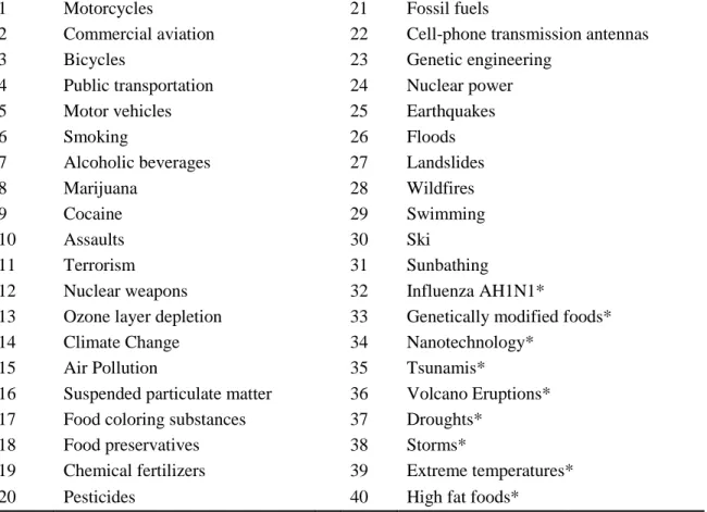
(21) 11. 3 3.1. METHODS AND DATA Instrument design. A survey including 40 hazards was designed, with 31 of them replicated from the preliminary study of Bronfman and Cifuentes (2003), and the other nine were related to new technologies, social ills and natural disasters that currently affect the country and were not included previously. The survey was designed to quantify eight risk attributes from the psychometric paradigm and three risk constructs (social risk, social benefit and social acceptability). All of these attributes and variables quantified social perceptions, that is, how participants perceive risks to be to the entire population, and not just to themselves. Additionally, nine questions were included to measure social trust. Of these questions, six of them were aimed at evaluating social trust (perceptions of competence and integrity) in 10 institutions responsible of risk communication regarding natural disasters, and the other three studied social trust in the participant’s community. In all questions associated to risk perception, the hazards were to be rated on a 7 point Likert scale, and questions regarding trust were to be rated on a 5 or 7 Likert scale, depending of the question. The survey was divided into three questionnaires: Form A included questions regarding the three analysis variables (and social trust questions), and forms B and C included 4 questions regarding the psychometric paradigm each. For the purpose of this study, which is to evaluate the evolution in perceptions of the Chilean population over the last decade, we will consider the 31 hazards that this study has in common with the study of Bronfman and Cifuentes (2003) and the 11 questions regarding risk perception (analysis variables and psychometric paradigm). Questions regarding social trust and the nine new hazards will be studied in further investigations, since they cannot be evaluated longitudinally at the time. The questions considered for this investigation and their distribution in the questionnaires can be observed in Table 3-1, and the 31 hazards (and the other 9 that were part of the survey) can be observed in Table 3-2. Additional. questions. sociodemographically.. were. also. included. to. characterize. the. participants.

(22) 12. Table 3-1. Attributes and analysis variables included in each questionnaire Variable. Scale end points. Description. Form. Low (1). High (7). Social risk. To how much risk is the national population subjected product of (……)?. No risk. High risk. A. Social benefit. How much benefits does the national population obtain product of (……)?. No benefit. High benefit. A. Social acceptability. How acceptable is the risk that affects the national population product of (……)?. Unacceptable. Acceptable. A. Novelty. Is the risk associated to (……) new and nonfamiliar, or is it old and familiar?. New. Old. B. Involuntariness. To what degree is the risk associated to (……) faced voluntarily by the exposed population?. Voluntary. Involuntary. B. Catastrophic potential. To what magnitude (……) has the potential to cause death and catastrophic destruction?. No catastrophic potential. High catastrophic potential. B. Dread. Is the risk associated to (……) a common risk or a terrible risk?. Common. Dread. B. Immediacy of the effects. Are the effects of the risk associated to (……) immediate, or do they take place later in time?. Immediate. Delayed. C. Severity of the consequences. When the risk associated to (……) appears: how likely is it that the consequences are fatal?. Non-fatal. Fatal. C. Social knowledge. In what degree is the risk associated to (……) known by the exposed population?. No knowledge. High knowledge. C. Social controllability. In what degree can the risk associated to (……) be controlled by the exposed population?. Not controllable. Highly controllable. C. Source: own elaboration.

(23) 13. Table 3-2. List of hazards evaluated. 1 2 3 4 5 6 7 8 9 10 11 12 13 14 15 16 17 18 19 20. Motorcycles Commercial aviation Bicycles Public transportation Motor vehicles Smoking Alcoholic beverages Marijuana Cocaine Assaults Terrorism Nuclear weapons Ozone layer depletion Climate Change Air Pollution Suspended particulate matter Food coloring substances Food preservatives Chemical fertilizers Pesticides. 21 22 23 24 25 26 27 28 29 30 31 32 33 34 35 36 37 38 39 40. Fossil fuels Cell-phone transmission antennas Genetic engineering Nuclear power Earthquakes Floods Landslides Wildfires Swimming Ski Sunbathing Influenza AH1N1* Genetically modified foods* Nanotechnology* Tsunamis* Volcano Eruptions* Droughts* Storms* Extreme temperatures* High fat foods*. Note: hazards with (*) were not considered in the 2001 survey Source: own elaboration. 3.2. Instrument validation. The questionnaire was validated through focus group sessions, conducted by the researchers and a sociologist in June 2013. For each questionnaire, a focus group was developed to measure the time length of each questionnaire and to see if the questions were easily understood. Considering that the study would cover a representative sample of Santiago’s population, it was decided to use a sub sample of six to eight individuals per focus group, where three criteria were considered in selecting the individuals. Males and females had to be represented in equal number, and four different age groups were established (from 18 to 30 years old, 31 to 45 years old, 46 to 60 years old and over 60 years old) where all categories had to be represented by at least one participant (ideally.

(24) 14. two). Since the lowest socioeconomic groups tend to have the poorest quality of education in the country, people belonging to socioeconomic groups C3 and D were selected in order to verify the clarity of the questions of the survey and the time taken to answer them. It was assumed that, if participants with the lowest educational levels in the country could answer the survey without problem, people with higher income and education would comprehend them as well. An introduction was included in the three questionnaires, informing of the content of the survey and the list of hazards. Additionally, an example was included for the three questionnaires to make it easier to respond the questions. Subjects took 20-30 minutes to answer questionnaire A and 15-20 minutes to answer questionnaires B and C. In general, there were no problems with understanding the questions and hazards, with the only exception of the hazards “Nanotechnology” and “Genetic Engineering”, were 50% of the participants of the focus groups claimed to be unfamiliar with them. These technologies were still included in the survey due to the numerous applications of them in Chile (computers and hard drives, cleaning products, frost resistant crops, etc.). For form A (analysis variables), subjects considered the example very helpful to understand the survey, however, for forms B and C (psychometric paradigm) it was considered confusing and not helpful at all. For these reasons, the example was only included in form A. A team of psychologists of Pontificia Universidad Católica that revised the survey also validated the instrument. Annex E shows the final questionnaires that were implemented. 3.3. Instrument Implementation. With the information provided by the National Institute of Statistics (INE)(Instituto Nacional de Estadísticas), 40 blocks were randomly selected from Santiago’s street map, where the four socioeconomic groups were equally characterized (10 blocks per socioeconomic level). A theoretical sample of a minimum of 384 participants was established per questionnaire that had to be representative of Santiago’s population. To achieve this, the population was segmented by gender, socioeconomic status (ABC1, C2,.

(25) 15. C3 and D) and age group (18 to 29 years old, 30 to 35 years old, 46 to 60 years old, and over 60 years old). To reach the number of participant needed, a minimum quota of 12 participants per gender, socioeconomic level and age group had to participate in the survey. Between July and September, a team of surveyors was hired and trained by the researcher in order to obtain the number of surveys required to achieve representation of the population. Through two training sessions and daily meetings, surveyors learned how to properly administer the survey to the population. The procedure to lift the information for each questionnaire (independently) began in the North-West corner of each block, where subjects were contacted in their households and had to answer the printed survey face to face. Surveyors were allowed to interview only one person per household and had to complete a quota of 12 surveys per block. In case they couldn’t complete the required amount of surveys, an adjacent block of similar characteristics was assigned to complete the quota. Subjects took 25-35 minutes to answer questionnaire A and 10-20 minutes to answer questionnaires B and C. Even though 384 surveys was the ideal quota per questionnaire, surveyors were asked to do a larger number of surveys (around 460) in order to eliminate possible outliers later. The sample obtained through this process is shown in Table 3-3..

(26) 16. Table 3-3: Sample obtained per questionnaire Form. 18 to 29 years old. 30 to 45 years old. 46 to 60 years old. Over 60 years old. Male. Female. Male. Female. Male. Female. Male. Female. ABC1. 15. 15. 15. 13. 11. 13. 12. 12. C2. 12. 13. 14. 15. 19. 15. 12. 16. C3. 13. 12. 13. 14. 12. 19. 12. 18. D. 14. 12. 14. 20. 13. 16. 17. 14. ABC1. 12. 12. 12. 12. 10. 14. 13. 14. C2. 14. 13. 13. 15. 15. 12. 13. 15. C3. 16. 14. 15. 18. 15. 17. 13. 16. D. 15. 11. 14. 14. 13. 15. 13. 14. ABC1. 14. 14. 13. 15. 14. 14. 12. 12. C2. 13. 15. 15. 13. 14. 20. 13. 19. C3. 14. 13. 13. 15. 14. 16. 14. 13. D. 14. 16. 16. 16. 14. 15. 16. 16. S.E. status. A. B. C. Source: own elaboration. A total of 1,381 surveys were obtained through this procedure, which were later digitalized in Excel and thoroughly revised by the researcher. Mean values and standard deviations were obtained for each question. Respondents who were outside the 95% confidence interval for more than 10% of the questions were considered outliers and purged from the sample. 108 participants were removed from the total sample in this process. 3.4. Data Analysis. The data was analyzed with Excel and the statistical program SPSS17. To compare rating scales of social risk and benefit between the study of 2001 (measured with 10 point scales) and the current study, the scales of 2001 for these variables were converted to a 7 point scale. To study any potential biases between the samples of 2001 and 2013 due to age differences, Tukey’s HSD tests were performed by hazard and year. Normality of the data was verified with quantile plots (Q-Q plots), and Levene’s test was run to study homogeneity of variances. Reliability of the psychometric scales was measured with Cronbach’s alpha (Cronbach, 1951), and confirmatory factor analysis.

(27) 17. was performed using Principal Components Analysis (PCA) with varimax rotation, where main factors and the cognitive map were extracted. OLS regression models were used to relate main factors with the three analysis variables (social risks, benefit and acceptability), and perceptions between genders and between years were compared through Independent Samples T-Tests. The different methods and techniques are further explained below. 3.4.1. Tukey’s HSD Test. The purpose of Tukey’s HSD test is to determine which groups in a sample have significant differences. This test is performed after an ANOVA test, and works by defining an HSD value (honest significant difference), that represents the minimum distance between two group means that must exist before two groups can be considered significantly different. 3.4.2. Normal probability Q-Q plot. Quantile plots (Q-Q plots) are a graphical technique used to determine if a dataset comes from a theoretical probability distribution or if two datasets come from populations with a common distribution (specified or unspecified).. These plots are built with the. quantiles of a certain dataset against the quantiles of another dataset (or theoretical distribution). A special case of the quantile plot is the normal probability plot, were the normality of a certain data is assessed (the data is set against a theoretical normal distribution) (Heiberger & Holland, 2004). Since normality is one of the requirements to use a parametric test such as independent samples t-test, it is important to check if the data distributes in such way. The straightness of the Q-Q plot indicates the degree of agreement of the data with the theoretical distribution. If a dataset matches with a normal distribution, but has certain departures of normality, the plot will show certain variations: . S shape: distributions with thinner tails than a normal.. . Inverted S shape: distributions with heavier tails than a normal. . J shape: positive skewness.

(28) 18. . Inverted J shape: negative skewness. . Isolated points at the extreme: presence of outliers. 3.4.3. Levene’s Test of Equality of Variances. When the population variances of two groups are equal, you have homogeneity of variances or homoscedasticity. Even though the violation of this assumption is not too serious, it is important to check it through Levene’s test in order to interpret properly the results of an independent samples T-test. If samples have homogeneity of variances, you must consider independent samples t-test calculated with pooled variances, and if the assumption is violated you consider results of the t-test with separate variances (nonpooled). 3.4.4. Principal Components Analysis. Principal components analysis (PCA) is a multivariate technique that reduces a large set of variables into a smaller set of uncorrelated variables (main factors or principal components), explaining as much of the variance as possible. These main factors are a linear combination of original variables (Dunteman, 1989). The goals of PCA are to reduce the dimensionality of the original data set, simplify the description of the data and analyze the structure of the variables (Abdi & Williams, 2010). In this study, main factors were extracted from the mean scores per hazard for the scales of the psychometric paradigm (quantified by participants in questionnaires B and C). To ensure the proper use of this technique, Kaiser-Meyer-Olkin (KMO) Measure of Sampling Adequacy for the overall data set and Bartlett’s test of sphericity were implemented. 3.4.4.1 KMO Measure of Sampling Adequacy The KMO measure is used as an index to determine if variables have a linear relationship between them and if PCA is appropriate to run on the data. Its value can range from 0 to 1, with values above 0.6 suggested as a minimum requirement for sampling adequacy. In this case, the KMO measure was 0.715, which is considered appropriate for the use of PCA, according to (Kaiser, 1974)..

(29) 19. 3.4.4.2 Bartlett’s Test of Sphericity The null hypothesis of this test is that there are no existing correlations between any of the variables, which would mean that the correlation matrix is an identity matrix. It is important to run this test before using PCA because, if there were no correlations between variables, it would be impossible to reduce them into a smaller number of components. Clearly, you want to reject the null hypothesis of this test in order to perform PCA. In this case, Bartlett’s Test of Sphericity was statistically significant (p<0.0005) indicating that the data was likely factorable. 3.4.5. OLS Regression Model. This type of regression model allows you to predict a dependent variable based on one or more independent variables. Through OLS regression models, you can determine the overall variance explained of the model and the contribution each of the independent variables (predictors) to the total variance explained. 3.4.6. Independent Samples T-Test. The independent-samples t-test determines if there are statistical significant differences between mean values of two independent groups on a dependent variable. Differences in perceptions between men and women, and changes in risk, benefit and acceptability in the last decade for each hazard (and types of hazard) are determined through this test..

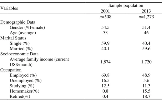
(30) 20. 4. RESULTS. 4.1. Sample population. 1,273 participants composed the sample. Each questionnaire was answered by a representative sample of Santiago, composed by 401 people in questionnaire A (M=47 years, SD=18 years, 52.3% women), 443 in questionnaire B (M=46 years, SD=18 years, 50.6% women), and 429 in questionnaire C (M=46 years, SD=18 years, 51.7% women). The final sample data is described in Table 4-1, along with the data from the study of 2001. Table 4-1. Description of Sample. Sample population 2001 2013 n=508 n=1,273. Variables Demographic Data Gender (%Female) Age (average) Marital Status Single (%) Married (%) Socioeconomic Data Average family income (current US$/month) Occupation Employed (%) Unemployed (%) Studying (%) Homemaker(%) Retired(%). 54.5 33. 51.4 46. 59.9 40.1. 40.4 59.6. 1,874. 1,720. 69.8 16.5 12.5 0.8 0.4. 48.9 5.6 11.3 15.5 18.7. Source: own elaboration. Considering that the mean age of the samples of 2001 and 2013 are rather different (33 and 46 years old), a Tukey’s HSD (honest significant difference) test was performed for each hazard per year, to observe if there were significant differences between age groups for mean values of social acceptability, risk and benefit. The purpose was to study the homogenous subsets of the test and determine if these age differences could be a bias for.

(31) 21. the study. The result of the test was that, for the majority of hazards, there were no significant differences in mean values for any of the groups. Only for a small group of hazards, significant differences between mean values were observed between the youngest and the oldest participants, but these groups had no significant differences with the other demographics. To illustrate this, Table 4-2 shows the homogenous subsets obtained for nuclear weapons and genetic engineering.. Table 4-2. Nuclear weapons and genetic engineering’s homogenous subsets for α = 0.05 (Tukey's HSD, dependent variable = social acceptability). Nuclear weapons 2001. Genetic engineering. 2013. 2001. Age Group. N. Set 1. N. Set 1. N. Set 1. 60-95 36-41 30-35 48-53 54-59 42-47 24-29 18-23. 4 19 28 7 9 13 65 28. 2 2.21 2.11 3.57 2.78 3.00 3.42 3.14. 91 35 38 38 39 36 54 38. 1.14 1.46 1.13 1.16 1.13 1.22 1.54 1.42. 4 18 29 7 10 14 65 28. 2.25 3.56 3.79 3.86 4.00 4.07. Sig.. 173. 0.683. 369. 0.087. 175. 0.195. 2013 Set 2 3.56 3.79 3.86 4.00 4.07 4.72 4.89 0.588. N. Set 1. 58 28 30 32 27 31 51 35. 3.24 3.32 3.57 3.44 2.89 3.74 3.57 3.37. 292. 0.463. Source: own elaboration. The case of nuclear weapons shows that all age groups have no significant differences in their mean scores, which is replicated for the majority of hazards. Mean values for acceptability regarding genetic engineering show that there are significant differences between 18-29 year old participants with 60-95 year old participants in the sample of 2001, which is a usual difference found when surveying a sample. Considering that the other hazards had similar results, this information indicates that, in general, participants of different age groups assess acceptability with no significant.

(32) 22. differences. Therefore, it is appropriate to compare the samples of 2001 and 2013 to study the evolution of perceptions in the last decade. 4.2. Transformation of Likert scales. In 2001, all variables and risk attributes were rated on a 7 point Likert scale, with exception of social risk and benefit which were rated on a 10 point scale. To compare the data of both years (in 2013 all variables were measured on 7 point Likert scales), all variables must be on scales with the same length. Following the recommendations of the study by (Colman et al., 1997), a linear transformation was used to convert the data of 2001 for social risk and benefit to a 7 point scale. The transformation equation applied to the data of 2001 is shown below: (. ). (1). In this equation, the ‘x’ represents the scores of the 10 point Likert scale and the ‘y’ represents the converted scores to a 7 point Likert scale. A correlation of 0.900 can be found between the original and the tranformed data of social risk, and, for social benefit, a correlation of 0.964 can be found between the original and transformed data (both values being significant at the 0.01 level). With these transformations, the pattern of results is very similar to the original data set and to standarized data, reflecting that it is appropiate to use the transformed data to analyze the evolution of risk and benefit perceptions between years. 4.3. Normality of the data. In order to compare perceptions between years with parametric tests, the assumption of a normal model must be met. For each year, the three analysis variables were tested for normality with normal probability Q-Q plots. In these plots, the data for the three variables appeared very similar to the theoretical normal distribution, clearly indicating that the underlying population was normally distributed. A very subtle inverted S shape.

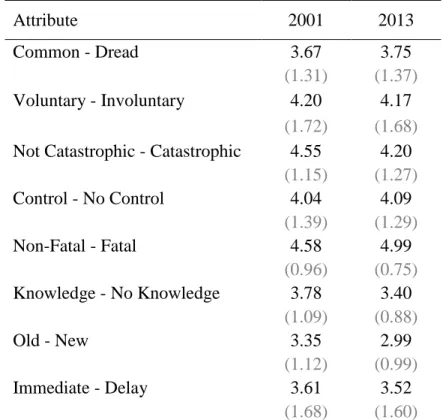
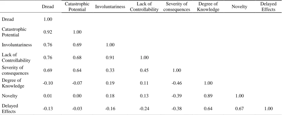
(33) 23. can be observed in all the plots, indicating slightly heavier tails in the datasets than in a theoretical normal distribution (to view the plots go to Annex A). 4.4. Homogeneity of variance. Homogeneity of variance was studied for each analysis variable with Levene’s test for equality of variances, where the variances of a hazard were compared between years for social risk, benefit and acceptability. In this process, it was determined that homogeneity differed between hazards and variables, with some hazards having homoscedasticity for one variable but not the other. Since this study compared mean values between years for each hazard with independent samples t-test, and this test offers two results for each hazard (assuming equal variances and not assuming equal variances), this is not an issue, and for every case the proper result was considered. 4.5. Description of Attributes. Considering the resulting factor structures obtained in the previous studies by Bronfman and colleagues, scale directions of social knowledge, control and novelty were inverted to have all attributes of a same factor with positive correlations (variables must measure a common entity in order to obtain positive alpha scores, which explains why they must correlate positively (Dixon, 2003; SAS Documentation, 2013)). “No knowledge”, “no controllability” and “new” became the high ends of the scales. Global mean values and standard deviations for each risk attribute are shown in Table 4-3, where it is observable that there are no significant changes in attribute scores between 2001 and 2013. When the population rates a hazard for its level of dread, this is highly correlated with the scores of catastrophic potential, lack of control, involuntariness and severity of consequences (see Table 4-4). On the other hand, scores of delayed effects, lack of knowledge and novelty have high correlations between them. For mean scores of risk attributes per hazard, go to Annex C..

(34) 24. Table 4-3. Mean values (standard deviations) for risk attributes in 2001 and 2013. Attribute. 2001. 2013. Common - Dread. 3.67 (1.31) 4.20 (1.72) 4.55 (1.15) 4.04 (1.39) 4.58 (0.96) 3.78 (1.09) 3.35 (1.12) 3.61 (1.68). 3.75 (1.37) 4.17 (1.68) 4.20 (1.27) 4.09 (1.29) 4.99 (0.75) 3.40 (0.88) 2.99 (0.99) 3.52 (1.60). Voluntary - Involuntary Not Catastrophic - Catastrophic Control - No Control Non-Fatal - Fatal Knowledge - No Knowledge Old - New Immediate - Delay. Note: no significant differences for any mean score between 2001 and 2013 Source: own elaboration.

(35) 25. Table 4-4. Correlation matrix of risk attributes (combined 2001-2013). Dread. Catastrophic Potential. Involuntariness. Lack of Severity of Controllability consequences. Degree of Knowledge. Novelty. Dread. 1.00. Catastrophic Potential. 0.92. 1.00. Involuntariness. 0.76. 0.69. 1.00. 0.76. 0.68. 0.91. 1.00. 0.69. 0.64. 0.33. 0.45. 1.00. -0.10. -0.07. 0.19. 0.11. -0.46. 1.00. Novelty. 0.01. 0.00. 0.18. 0.13. -0.39. 0.89. 1.00. Delayed Effects. -0.13. -0.03. -0.16. -0.24. -0.38. 0.64. 0.67. Lack of Controllability Severity of consequences Degree of Knowledge. Source: own elaboration. Delayed Effects. 1.00.

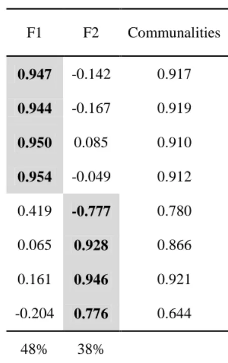
(36) 26. 4.6. Factor analysis. Based on a hazard x attribute rating matrix (created by averaging responses over participants), PCA was performed and a classic factor structure was obtained, accounting for 86% of sample’s variance (see Table 4-5). The first factor, labeled Dread Risk,. was composed of four attributes (social control, dread, voluntariness and. catastrophic potential). Severity, degree of knowledge, immediacy of effects and degree of novelty formed the second factor, labeled Unknown Risk. The only difference in relation to the factors obtained in 2001 was that the attribute “Severity of consequences” (Non-fatal to Fatal) switched from Factor 1 to Factor 2. This is not surprising since, in both years, this attribute correlates well with both factors.. Table 4-5: Rotated components matrix for each year 2001 Attributes Common - Dread Not Catastrophic Catastrophic Voluntary - Involuntary Control - No Control Non-Fatal - Fatal Knowledge - No knowledge Old - New Immediate - Delay. Total variance explained. 2013. F1. F2. Communalities. F1. F2. Communalities. 0.951. -0.074. 0.909. 0.947. -0.142. 0.917. 0.883. -0.035. 0.781. 0.944. -0.167. 0.919. 0.818. 0.172. 0.699. 0.950. 0.085. 0.910. 0.838. 0.128. 0.718. 0.954. -0.049. 0.912. 0.832. -0.315. 0.791. 0.419. -0.777. 0.780. 0.011. 0.960. 0.921. 0.065. 0.928. 0.866. 0.058. 0.933. 0.873. 0.161. 0.946. 0.921. -0.074. 0.832. 0.697. -0.204. 0.776. 0.644. 47%. 33%. 48%. 38%. Source: own elaboration.

(37) 27. 4.6.1. Combined Factor Analysis. Since there are no major differences between 2001 and 2013 in the composition of factors, a factor analysis was performed combining the information of 2001 and 2013, to observe the changes of each hazard in the cognitive map. This model explained 81% of sample’s variance and showed no relevant differences in composition with the factors previously obtained in this study (see Table 4-6). Internal consistency of the scales was studied through Cronbach’s alpha considering aggregated data by participants (matrix of scales and hazards). Factor 1 had an alpha of 0.935 and Factor 2 had an alpha of 0.838. (Nunnally & Bernstein, 1994) suggest a value of 0.70 as the lower acceptable bound for alpha, and (DeVellis, 2003) considers alpha ranges over 0.80 as “very good”, indicating that the scales obtained in this study are of a very high degree of reliability.. Table 4-6. Rotated components matrix for factor analysis 2001-2013. Attributes. F1. F2. Communalities. Common - Dread. 0.946. -0.112. 0.907. Not Catastrophic - Catastrophic. 0.899. -0.075. 0.814. Voluntary - Involuntary. 0.893. 0.134. 0.816. Control - No Control. 0.907. 0.045. 0.824. Non-Fatal - Fatal. 0.630. -0.544. 0.693. Knowledge - No knowledge. 0.046. 0.948. 0.900. Old - New. 0.107. 0.941. 0.897. Immediate - Delay. -0.141. 0.791. 0.646. 47%. 34%. Total variance explained. Source: own elaboration.

(38) 28. Source: own elaboration. Figure 4-1 shows the cognitive map for the 31 hazards and indicating their positions in 2001 and 2013. General tendencies regarding the positioning of hazards in the map have not been considerably altered through time. Aligned with results observed in the study by Slovic (1987) and colleagues, Factor 1 (“Dread Risk”) is defined at its high end by perceived catastrophic potential, dread, lack of control, involuntariness and fatal consequences (severity).. Factor 2 (“Unknown. Risk”) is defined at its high end by hazards that are judged as unknown, new and delayed manifestation of harm. An important observation that can be drawn from the cognitive map, is that the great majority of risks have lower scores in Factor 2 in 2013 than they did in 2001. This means that, in general, the population has a better understanding of risks and perceives them as older risks. Evidently, education has a very important role in this change of perception, since it provides the necessary tools for the population to understand risks. Most hazards remain in the same quadrants than a decade ago, showing that their relative positions have had no drastic alterations. Technological and environmental hazards are still located in the upper right quadrant, which is the quadrant with highest scores for “Dread Risk” and “Unknown Risk”. The level of dread that these hazards produce in the population is high, and it is very likely that more strict regulation to achieve risk reduction of these hazards is what the public wants (Slovic, 1987). Chemical products and substances (and one technological hazard) are located in the upper left quadrant, where there are high scores of “Unknown Risk” and low scores of “Dread Risk”. These hazards are perceived as more common, with lower perceptions of catastrophic potential and higher controllability than those positioned in the right upper quadrant. Natural disasters and social ills continue to be located in the lower right quadrant, which is where hazards with the highest scores of “Dread Risk” and lowest scores of.

(39) 29. “Unknown Risk” are positioned. Hazards that fall into this category have characteristics that make them well known and understood by the population but at the same time are.

(40) 30. Source: own elaboration Figure 4-1: Position of hazards in factorial map in 2001 and 2013 (movement shown by arrows).

(41) 31. perceived with high levels of dread, lack of control and catastrophic potential. Even though natural disasters had high scores for Factor 1 in 2001, they continue to move to the high extreme of the scale, and are perceived are more dreadful, catastrophic and less controllable than before. Finally, transport hazards, forbidden and addictive substances and other hazards fall in the lower left quadrant, where there are low scores for both factors. Hazards that are positioned in this quadrant represent those hazards that the population perceive as old risks with high degree of knowledge and control. Genetic engineering is still perceived in the highest position regarding Factor 2. After 12 years, floods, earthquakes, landslides, wildfires, terrorism and nuclear weapons continue to be perceived as the most dreaded hazards. By observing the cognitive map, it is clear that scores for “Unknown Risk” in 2013 are lower than those of 2001. The hazards with the most pronounced movements in the factor space (greater than 0.5 in a factor) were studied, in order to determine if their movements were because of changes in all attributes or because of a change in a particular set of attributes. For Factor 1, bicycles moved towards the right due to significantly higher scores in the severity of consequences attribute (+1.85)1 and lack of controllability (+0.84). Marijuana and cocaine have moved to the left due to significantly lower scores for catastrophic potential (-2.31 for marijuana and -2.12 for cocaine) and dread (1.53 for marijuana and 1.23 for cocaine). Wildfires have moved considerably to the right, and this movement is because scores for all attributes in Factor 1 have significantly increased for this hazard. Nowadays, the population perceives wildfires to be more dreadful, catastrophic, involuntary, severe and less controllable. Food coloring substances is the only hazard that shows large movements in both factors. For Factor 1, significantly higher scores can be observed in all attributes with exception of lack of controllability, explaining its movement towards the right end of the scale. For Factor 2, the population perceives to. 1. Changes in scores between 2001 and 2013 for the given attribute, on a 7 point Likert scale. A positive (negative) sign means that there is an increase (decrease) in an attributes’ score..

(42) 32. have a higher degree of knowledge of food coloring substances (+0.78), explaining why this hazard has moved to the lower end of the scale. Smoking and air pollution also show movements in this factor towards the lower end of the scale, which is explained by similar score differences between years in all the attributes that compose this factor (between |. |. |. | ). Both hazards are perceived today with higher degree of. knowledge, as older risks and effects are sensed as more immediate than before. Ozone layer depletion, sunbathing, cell phone transmission antennas and suspended particulate matter have moved in Factor 2 mainly because they are perceived as older risks and with greater degree of knowledge than before, with significant differences for these attributes between years (-1.16Novelty, -0.73Unknowledge for ozone layer depletion, -0.69. Novelty,. -. 0.78Unknowledge, for suspended particulate matter, -1.32Novelty, -0.95Unknowledge for cell phone transmission antennas and -1.29 Novelty, -0.93Unknowledge for sunbathing).. 4.7. Changes in male and female perceptions during the last decade. In a decade, risk perceptions have significantly changed in the Chilean population. With an improved quality of life, better education and opportunities, social acceptability and benefit perceptions are significantly lower and risk perceptions higher in 2013 than in 2001 for the total population..

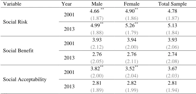
(43) 33. Table 4-7. Mean scores (standard deviations) for analysis variables in 2001 and 2013. Variable. Year 2001. Social Risk 2013 2001 Social Benefit 2013 2001 Social Acceptability 2013 **. Male 4.66 ** (1.87) 4.99** (1.88) 3.93 (2.12) 2.76 (2.05) 3.82** (2.00) 2.81 (1.89). Female 4.90** (1.86) 5.26** (1.79) 3.94 (2.00) 2.76 (2.11) 3.52** (2.04) 2.82 (1.99). Significant differences between genders of a same year at p<0.01. Source: own elaboration. Total Sample 4.78 (1.87) 5.13 (1.84) 3.93 (2.06) 2.74 (2.08) 3.67 (2.03) 2.81 (1.94).

(44) 34. As shown in Table 4-7, for each gender, mean values for risk, benefit and acceptability show significant differences (p<0.01) between 2001 and 2013. In general, both genders appreciate hazards today as less acceptable, with higher social risk and lower benefit perceptions. Women and men continue to perceive social risk significantly different in 2013, despite narrower differences in education than before. In 2001, significant differences in risk perceptions between genders could be observed for natural and technological hazards, forbidden or addictive substances, social ills and other hazards. Nowadays, these differences keep existing (with exception of natural hazards), and transport hazards, and chemical products and substances are also added to hazards where genders have significant differences for social risk. In benefit scores, males and females of 2001 show significant differences for transport and environmental hazards. In 2013, these differences keep existing and chemical products and substances and natural hazards are also perceived by males and females with significant differences. Acceptability scores show the opposite effect. In 2001, significant differences existed for forbidden or addictive substances, social ills, chemical products and substances, technological and natural hazards. The present situation has changed considerably, with men and women having very similar mean scores for acceptability in 2013 and no significant differences in their perceptions for all hazards, with exception of transport hazards (at p<0.05). Table 4-8 shows mean scores of risk, benefit and acceptability perceptions by gender and year..

(45) 35. Table 4-8. Mean scores for analysis variables by gender and year. Social Risk. Social Benefit 2013. 2001 Male Female. Male. Female. Transport hazards(b)(c) (d) (f). 3.65. 3.69. 3.96. Forbidden or addictive substances(a)(b)(e). 5.55. 5.91. Social ills(a)(b)(e). 5.56. Environmental hazards(c) (d) Chemical products and (b (d)(e) substances Technological hazards Natural hazards Other hazards. (a)(d)(e). (a)(b). (a) (b) (e). Social Acceptability. 2013. 2001 Male Female. Male. Female. 4.29. 5.73. 5.46. 5.22. 5.54. 5.82. 2.24. 2.09. 5.92. 5.66. 6.13. 1.81. 5.38. 5.47. 5.70. 5.83. 4.32. 4.33. 5.18. 4.14. 4.46. 5.33 3.36. 2013. 2001 Male Female. Male. Female. 5.40. 4.87. 4.69. 4.80. 4.96. 1.79. 1.68. 3.01. 2.50. 2.27. 2.30. 2.08. 1.17. 1.17. 2.84. 2.43. 1.26. 1.27. 1.54. 1.94. 1.57. 1.47. 3.03. 2.91. 1.80. 1.73. 5.37. 3.14. 3.15. 2.28. 2.10. 3.75. 3.47. 2.59. 2.52. 4.52. 4.94. 4.46. 4.36. 3.60. 3.42. 4.04. 3.66. 3.41. 3.30. 5.72. 5.88. 6.02. 1.42. 1.43. 1.26. 1.17. 3.71. 3.37. 1.48. 1.46. 3.79. 3.57. 3.84. 4.04. 3.98. 4.67. 4.82. 5.14. 4.93. 4.34. 4.55. (a). Significant differences between genders of 2001 for social risk at p<0.05. Significant differences between genders of 2013 for social risk at p<0.05. (c) Significant differences between genders of 2001 for social benefit at p<0.05. (d) Significant differences between genders of 2013 for social benefit at p<0.05. (e) Significant differences between genders of 2001 for social acceptability at p<0.05. (f) Significant differences between genders of 2013 for social acceptability at p<0.05. (b). Source: own elaboration.

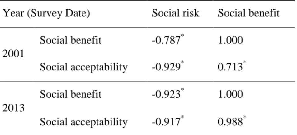
(46) 36. Very high correlations between risk, benefit and acceptability can be observed in Table 4-9. Benefit and acceptability have a positive correlation between them, while risk has a negative correlation with the two other variables.. Table 4-9: Bivariate correlation between social risk, social benefit and social acceptance. Year (Survey Date). Social risk. Social benefit. Social benefit. -0.787*. 1.000. Social acceptability. -0.929*. 0.713*. Social benefit. -0.923*. 1.000. Social acceptability. -0.917*. 0.988*. 2001. 2013. * Indicates p<0.01 for the correlation being equal to zero. Source: own elaboration. 4.8. Relationship between factors of the psychometric paradigm and perceptions of analysis variables. OLS regression models were run to predict perceived social risk, benefit and acceptability from Factor 1 and Factor 2. The assumptions of linearity, independence of errors, unusual points and normality were met. Only Factor 1 predicted the three variables with statistical significance (p<0.05). For both years, higher scores in Factor 1 relate with an inequitable distribution of risks and benefits (high risks and low benefits), which lead as well to a low perception of acceptability. Regression coefficients and significance levels can be found in Table 4-10..

(47) 37. Table 4-10. Standarized coefficients from OLS regression models Dependent variables. Year 2001. Social Risk 2013 2001 Social Benefit 2013 2001 Social Acceptability 2013. Independent variables Factor 1: Dread Risk Factor 2: Unknown Risk Factor 1: Dread Risk Factor 2: Unknown Risk Factor 1: Dread Risk Factor 2: Unknown Risk Factor 1: Dread Risk Factor 2: Unknown Risk Factor 1: Dread Risk Factor 2: Unknown Risk Factor 1: Dread Risk Factor 2: Unknown Risk. Beta 0.69 -0.05 0.53 -0.13 -0.51 -0.05 -0.59 -0.03 -0.59 -0.20 -0.67 -0.01. Standarized coefficients t p-value 5.08 0.00 -0.35 0.73 3.36 0.00 -0.80 0.43 -3.18 0.00 -0.34 0.74 -3.83 0.00 -0.23 0.82 -3.96 0.00 -1.33 0.20 -4.72 0.00 -0.07 0.95. Source: own elaboration. 4.9. Changes in social perceptions analyzed by type of hazard. Table 4-11 shows mean scores of risk perceptions by type of hazard. In general, risk perception of today’s population has become higher than it was a decade ago, with the exception for the groups of forbidden and addictive substances, social ills and other hazards. Natural hazards have the highest risk perceptions for 2013, which significant changes from 2001 (. ). The largest difference in risk perceptions can be. observed for the group of chemical products and substances (. )..