Decoherence in generalized measurement and the quantum Zeno paradox

Texto completo

(1)Physics Reports 540 (2014) 1–23. Contents lists available at ScienceDirect. Physics Reports journal homepage: www.elsevier.com/locate/physrep. Decoherence in generalized measurement and the quantum Zeno paradox Gerhard Mack a , Sascha Wallentowitz b , Peter E. Toschek c,∗ a. II. Institut für Theoretische Physik, Universität Hamburg, Luruper Chaussee 149, D-22761 Hamburg, Germany. b. Facultad de Física, Pontificia Universidad Católica de Chile, Casilla 306, Santiago 22, Chile. c. Institut für Laser-Physik, Universität Hamburg, Jungiusstr.9, D-20355 Hamburg, Germany. article. info. Article history: Accepted 9 February 2014 Available online 18 February 2014 editor: J. Eichler Keywords: Quantum measurement Decoherence Quantum Zeno paradox. abstract In the development of quantum mechanics, the evolution of a quantum system was a controversial item. The duality of unitary evolution and state reduction as proposed by John von Neumann was widely felt unsatisfactory. Among the various attempts to reconcile the two incompatible modes of dynamics, the model of decoherence has turned out rather convincing. While the debate has been going on mainly by reasoning the consequences of gedanken experiments, the technical progress has made available techniques of addressing real experiments, even on an individual quantum object. In particular, the impeded evolution of an atom under continuous or reiterated measurement, predicted long ago, has been proven. The procedure of such an experiment – as with many a more conventional one – includes sequences of alternating time intervals of preparation and detection, known as ‘‘pump–probe’’, or ‘‘drive–probe’’ measurements. We discuss this procedure in the context of the decoherence model. The emergence of pointer states of the meter is outlined. We show compatibility of this approach with photon counting, and emphasize the importance of information transfer in the course of measurement. Qualitative conditions having been considered so far necessary and sufficient criteria for meeting the ‘‘quantum Zeno paradox’’ are being quantified. © 2014 Elsevier B.V. All rights reserved.. Contents 1. 2.. 3.. ∗. Introduction............................................................................................................................................................................................. A measured quantum system................................................................................................................................................................. 2.1. The model.................................................................................................................................................................................... 2.2. The unitary time evolution ........................................................................................................................................................ 2.3. The interaction of system and environment simulator............................................................................................................ 2.4. Generalized measurements on system A .................................................................................................................................. A system with a meter immersed in an environment .......................................................................................................................... 3.1. Environment simulator as a meter in an environment of its own .......................................................................................... 3.2. A two-level system and its one-qubit meter ............................................................................................................................ 3.3. The reduced density matrix for system and meter .................................................................................................................. 3.4. Reading the meter ....................................................................................................................................................................... Corresponding author. Tel.: +49 40428382381; fax: +49 40428386571. E-mail address: toschek@physnet.uni-hamburg.de (P.E. Toschek).. http://dx.doi.org/10.1016/j.physrep.2014.02.004 0370-1573/© 2014 Elsevier B.V. All rights reserved.. 2 3 3 4 4 5 5 5 6 7 7.

(2) 2. G. Mack et al. / Physics Reports 540 (2014) 1–23. 4.. 5.. 6. 7. 8. 9.. 10. 11.. Evolution determined by reiterated measurement .............................................................................................................................. 4.1. Quantum Monte Carlo trajectories ............................................................................................................................................ 4.2. Evolution of the modeled system and meter ............................................................................................................................ 4.3. The probability distribution of light scattering ........................................................................................................................ Fluorescence probing of a coherently prepared three-level atom....................................................................................................... 5.1. The system .................................................................................................................................................................................. 5.2. Coupling of system and meter ................................................................................................................................................... 5.3. Detection and read-out .............................................................................................................................................................. 5.4. Successive cycles of measurement ............................................................................................................................................ The quantum Zeno effect........................................................................................................................................................................ The emergence of pointer states: absorptive probing .......................................................................................................................... Dynamics and information in one drive–probe measurement............................................................................................................ Information, selectivity, and the QZP .................................................................................................................................................... 9.1. Information from a series of drive–probe measurements ....................................................................................................... 9.2. Flow of information and the quantum Zeno paradox .............................................................................................................. Summary ................................................................................................................................................................................................. Conclusions.............................................................................................................................................................................................. Acknowledgment .................................................................................................................................................................................... Appendix. Evaluation of the probability Nk of a sequence of no-clicks ......................................................................................... A.1. The diagonalization and exponentiation of a traceless 2 × 2 matrix ..................................................................................... A.2. The trace of matrix M = −iHA /h̄ − J ........................................................................................................................................ References................................................................................................................................................................................................. 7 7 7 8 8 9 10 11 13 14 15 17 17 17 18 20 20 21 21 21 21 22. 1. Introduction During the past decades, sophisticated novel techniques for the preparation and manipulation of matter and radiation fields have allowed the experimentation with individual ions [1], neutral atoms [2,3], and single-mode fields [4,5]. These achievements have rekindled the simmering debate on the foundations of quantum mechanics, since quite a share of the early gedanken experiments seem addressable today in experiment, or have been done so already. One of the central problems concerns the process of measurement on a microscopic object, and consequently the interaction of a macroscopic apparatus with an object subjected to quantum mechanics [6]. A particularly controversial ingredient of the quantum evolution of an observed system was the requirement to accept two, as it seems, incompatible modes of evolution: the deterministic unitary evolution of the system, governed by the Schrödinger equation, and the ‘‘state reduction’’, taking place after a recorded observation of typically random results [7]. Novel concepts have stressed the action of the environment on both the observed quantum system and the measuring device, the ‘‘meter’’, and have elucidated important aspects of quantum evolution [8]. These concepts have matured up to a level that promises useful applications to the interpretation of real experiments on a quantum system, including recorded data. A characteristic example of a problem accessible by contemporary experiments, and closely related to the question of quantum measurement, is the inhibition of the quantum evolution by the system’s continuous or reiterated observation predicted long ago [9–11]. For the demonstration of this ‘‘quantum Zeno paradox’’ (QZP), a system seems appropriate that is represented by an evolving pseudo-spin 1/2, i.e., a driven two-level system. With such a system the occupation of one of two active levels was suggested to be probed by recurrent excitation on an adjacent strong line [12]. Certain observations on ensembles of such systems, i.e. clouds of trapped ions [13] (see also [14,15]) have yielded results in agreement with predictions from quantum mechanics. They have been claimed to demonstrate the quantum Zeno effect (QZE). However, the interpretations of these experiments have been challenged for not measuring the survival of the system in its initial state [16], for possible dynamic back action of the meter on the quantum system, i.e. lacking the quality of quantum non-demolition (QND) [17], and for the use of non-selective measurements, i.e., the detection of expectation values from the ensembles of objects, instead of eigenvalues, as from an individual object [17]. Consequently, the results of such measurements seem necessary for the presence of a QZE, but not sufficient, as they are with a selective QND measurement of survival on an individual quantum object. The conceptually simplest measurement of an observable of a microscopic object is a ‘‘yes-or-no’’ interrogation of one state of an individual pseudo-spin 1/2 system, since the relevant Hilbert space is two-dimensional, and the possibly extracted information is just one bit. More measurements are required when the observations are to be compared with a quantummechanical expectation value of the observable, which here relates to an ensemble of observations, not of objects. Each of these interrogations consists of suitably probing one of the two energy eigenstates, e.g. by the attempt of exciting light scattering from the system in the corresponding state. If the system has been initially in the probed eigenstate or in the opposite one, results of this repeated probing form a sequence of only ‘‘yes’’ (1) or only ‘‘no’’ (0) data, respectively. When shifted, by a preceding driving pulse, into a superposition state, the system will respond to interrogation of its state occupation – that formally represents the pseudo-spin vector’s z component – by making yield the meter a conditionally random result 1 or 0, that goes along with state reduction of the system. Assume the initial state was 0. Then, this result signals ‘‘survival’’, result 1 ‘‘transition’’ of the system. When 0 has been found, another coherent preparation of the system by the next (equal) driving pulse generates an identical unitary rotation trajectory..

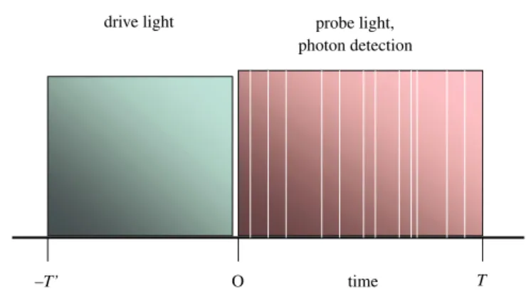
(3) G. Mack et al. / Physics Reports 540 (2014) 1–23. 3. Pump-probe measurement drive light. –T’. probe light, photon detection. O. time. T. Fig. 1. Drive–probe measurement. Detection of probe-induced fluorescence pulses; alternative single-photon detection of fluorescence or detection of absorption.. A few years ago, results in form of bit sequences have become available from measurements on a well defined quantum system, namely an individual ion stored in the isolating environment of an electrodynamic trap [18–20]. It has been pointed out that such measurements meet the stringent criteria for the observation of the QZE, and even of the quantum Zeno paradox [17]. On the other hand, this suppression of the temporal evolution of a quantum system by measurement requires detailed analysis since it has been ascribed so far to various phenomena, e.g. decoherence [21], or back action of the meter upon the system, as it had been invoked for the initial explanation of complementarity [22]. The present work aims to gain more profound understanding of the above procedure of preparation and measurement on an individual quantum object by analyzing this procedure in terms of the decoherence hypothesis [23–25]. This task seems the more appropriate as the reiterated driving and probing represents the simplest non-trivial combination of preparation and observation, known as ‘‘pump–probe’’, or ‘‘drive–probe’’ measurement (Fig. 1). We show the respective roles of environment and meter, and outline the emergence of the meter’s ‘‘pointer states’’ in the above and related scenarios. The consequences of ‘‘read’’ and ‘‘unread’’ measurements for this strategy are pointed out. A useful characterization of the recorded data set is the information accumulated either by photon counting during probing, or by recording just one result per probe interval in the sequence of subsequent measurements. In Section 2, a two-level system interacting with an ‘‘environment simulator’’ is modeled. The simulator represents a particular mode of the radiative environment which may act as the quantum sensor of the meter, as in the application addressed later, laser-induced fluorescence is being detected. Thus, the meter is represented by part of the environment of the system, a particular mode of the electromagnetic field. The structure of a generalized measurement is analyzed. Section 3 extends this model to including a meter with an environment of its own, and gives the resulting master equation. The role of a photon counter is discussed. Section 4 describes the derivation of quantum jump trajectories for the evaluation of the statistics of recordings. A three-level atom is addressed in Section 5 in order to allow for a more general preparation preceding the probing, and matching the procedure of previous experiments. In Section 6, QZE and QZP are outlined in the given context. Section 7 describes an arrangement where, for the probing, light scattering by the atom is replaced with the atom’s absorption as the meter signal. Finally, the flow of information is considered: within a drive–probe cycle (Section 8), and at the end of a sequence of drive–probe cycles (Section 9). 2. A measured quantum system 2.1. The model We consider a quantum system A whose non-degenerate states form a Hilbert space H A and a qubit B, whose states are assumed to form a 2D Hilbert space H B . We identify B with an ‘‘environment simulator’’ (Fig. 2). Measurements in B are envisaged of some observable O : H B → H B . Accordingly, there is a distinguished basis in H B which consists of eigenvectors, |eb ⟩ ∈ H B of O with the ground state |e0 ⟩ = |0(B) ⟩ (off), and an excited state |e1 ⟩ = |µ(B) ⟩ (on), where µ = 1. The Hilbert space of system + environment simulator is H B ⊗ H A . For the moment we consider a unitary evolution in A that involves a trivial Hamiltonian HA = 0, and there be only one Lindblad operator Lµ : H A → H A , which enters the master equation for the reduced density matrix ρA of the system A [26]. The problem is to find a unitary time evolution U (τ ) : H B ⊗ H A → H B ⊗ H A. (1). for system + environment simulator (possibly a meter) which reproduces the master equation for ρA . A and B turn out entangled, at the end of the time interval τ . An unread measurement on B erases this entanglement and leaves A in a (more).

(4) 4. G. Mack et al. / Physics Reports 540 (2014) 1–23. a. b. c. Fig. 2. Schemes of coupling an atom to meter and environment: a: Atom coupled to a meter represented by an environment simulator. b: Atom coupled to meter immersed in environment of its own. c: Atom coupled to meter made up of a qubit coupled to a macroscopic detector.. mixed state. On the other hand, a read-out measurement projects A onto a new state vector that may be taken as initial state for the next step of the evolution. 2.2. The unitary time evolution Expanding in the basis |eb ⟩ for H B we may write, for arbitrary |Ψ ⟩ ∈ H A , U (τ )(|ea ⟩ ⊗ |Ψ ⟩) =. . |eb ⟩ ⊗ Uba |Ψ ⟩. (2). b. with a 2 × 2 matrix U whose entries Uba are operators in H A . We want to describe the evolution of system A by expanding U after the lapse of a time increment τ in terms of one time-independent Lindblad operator Lµ . To first order in τ , U(τ ) = with J =. . 1 ∗ L L 2 µ µ. 1 − τJ. √. τ Lµ. and J̃ =. √  − τ L∗µ , 1 − τ J̃ 1 L L∗ . 2 µ µ. (3). One verifies by matrix multiplication that the block matrix U(τ ) is unitary to order τ ..  (Uba )∗ Ubc = δac + o(τ ).. (4). b. It follows from the naming of states |eb ⟩, Eqs. (2) and (3), that U (τ )(|0(B) ⟩ ⊗ |Ψ ⟩) = |0B ⟩ ⊗ (1 − J τ )|Ψ ⟩ + |µ(B) ⟩ ⊗. √ τ Lµ |Ψ ⟩,. (5). in agreement with Eq. (4.66) [26]. In addition we get U (τ )(|µ(B) ⟩ ⊗ |Ψ ⟩) = |µ(B) ⟩ ⊗ (1 − J̃ τ )|Ψ ⟩ − |0(B) ⟩ ⊗. √ ∗ τ Lµ |Ψ ⟩. (B). The unitary time evolution makes transitions from meter state |0. (6) (B). (B). (B). ⟩ to |µ ⟩ and also from |µ ⟩ to |0 ⟩!. 2.3. The interaction of system and environment simulator Consider the following transition operators in H B :. σ+B = |µ(B) ⟩⟨0(B) |,. σ−B = |0(B) ⟩⟨µ(B) |.. (7).

(5) G. Mack et al. / Physics Reports 540 (2014) 1–23. 5. Now we can write U (t ) = exp. . −i h̄.  HI t. (8). for arbitrary t, with.  ih̄  HI = √ σ+B Lµ − σ−B L∗µ .. (9). τ. This Hermitian operator in H B ⊗ H A may account for the fluorescent decay of an atom plus its reexcitation necessary for keeping flow equilibrium in the open system. By power series expansion of the exponential in Eq. (8) to second order one verifies that the block matrix form of U (τ ) agrees with (3) to order τ . The correctness of Eq. (8) for all t follows from the product law for exponentials. This also furnishes an alternative proof of the unitarity of U (τ ) as defined by Eq. (3). Up to now, the Hamiltonian for the system A has been assumed to be 0. Otherwise, Eq. (8) has to be replaced by U (t ) = exp. . −i h̄. . [H + HI ]t . A. (10). The usual type of measurement on a system made up of an unstable atom is based on the detection of fluorescence photons. Now, a corresponding Hamiltonian HI = ih̄Γ σ+ Lµ , is non-Hermitian, since fluorescent decay is irreversible, and the evolution is not unitary. However, resetting B to its distinguished state |0B ⟩ after a time increment τ ≈ Γ −1 , where Γ is the decay rate of the excited light mode, leaves the evolution approximately unitary and vindicates Eq. (9). 2.4. Generalized measurements on system A A generalized measurement M (positive operator-valued measurement, POVM) on system A requires the state of A to become entangled with a meter qubit (ancilla), as which may serve here the environment simulator B. This operation is defined by a set of not necessarily Hermitian Kraus operators Mµ [27], in arbitrary number, including M0 which plays a distinguished role later on, and with normalization M0∗ M0 +.  µ̸=0. Mµ∗ Mµ = 1.. (11). The entangling evolution extends over a short time interval τ . The Lindblad operators Lµ = L(µA) considered later are related to Mµ by. √ τ Lµ , µ ̸= 0  L∗µ Lµ . M0 = 1 − τ Mµ =. (12) (13). µ̸=0. At the beginning of the time interval, the meter qubit B is supposed to be in the distinguished state |0(B) ⟩. Then the system and the ‘‘meter’’ (the environment simulator) get entangled by a unitary time evolution UM , as described before, with Lµ and Mµ related as in Eq. (12). At the end of the time interval, an unread measurement on B is made. It may involve the interaction of this meter qubit with its own environment (Fig. 2b), or with a photon counter which is part of this environment, and whose clicks are possibly recorded (Fig. 2c). The required resetting of the meter qubit B is then formally retraced to these interactions. The generalized measurement may be reiterated after subsequent time increments τ that should exceed the correlation time τc of this environment. 3. A system with a meter immersed in an environment 3.1. Environment simulator as a meter in an environment of its own We shall now set up a model where the environment simulator B is characterized by a Hilbert space H B spanned by a distinguished ground state |0B ⟩ ∈ H B , and a finite number of other states |µB ⟩ ∈ H B and by Lindblad operators Lµ that act in the system’s Hilbert space H A for every µ ̸= 0, and a time scale τ (Fig. 2b). The simulator qubit is now considered to act as a meter of the system. The resetting of this meter to |0⟩ is dictated by the requirement that the meter has no memory. Otherwise, what the meter indicates would not be determined by the state of the system alone but also by the system’s history. In order to elucidate the emergence of ‘‘pointer states’’ that represent the alternative results of this measurement, the coupling of B to an environment of its own seems adequate. The effect of the environment can be summarized by new Lindblad operators LB which enter the Lindblad equation for the reduced density matrix of system + meter. They act on.

(6) 6. G. Mack et al. / Physics Reports 540 (2014) 1–23. H B ⊗ H A by acting on H B . The necessity of setting back the meter to state |0(B) ⟩ after each decay of the system’s excited state suggests that the natural Lindblad operators are. √ Γ |0(B) ⟩⟨µ(B) |,. LBµ =. (14). µ ̸= 0 characterizes the excited states, and Γ determines the decay time τes of the environment simulator; presumably Γ = τes−1 up to a factor around 1. This model would explain the appearance of ‘‘pointer states’’ |0(B) ⟩, |µ(B) ⟩ of the meter. They are determined by the coupling of the system to the meter via an interaction Hamiltonian HI (which is given by Eq. (9)); this introduces the operators Lµ , and the fixing of a distinguished state |0(B) ⟩ of the meter. Thus, natural pointer states of the meter emerge [28], and the Lindblad operator for the meter destroys excitations of the meter. The Lindblad equation for the reduced density matrix ρ AB of system + meter reads dρ AB (t ) dt. i. = − [H + HI , ρ ] + A. AB. h̄.  µ̸=0. AB BĎ. Lµ ρ Lµ − B. 1 2. BĎ B. Lµ Lµ ρ. AB. 1. AB BĎ B. . − ρ Lµ Lµ . 2. (15). This master equation for the density matrix ρ AB (t ) of the coupled system A and meter B can be understood as a consequence of the interaction of the system A (with Hilbert space of states H A ) with an environment simulator B (with Hilbert space of states H B ) [26, section 4.3.3]. It is an essential feature of the scheme that there is a distinguished neutral state |0⟩ ∈ H B and that B is reset to |0⟩ after every time interval τ , since the meter is considered to lack a memory. In between, the state of B gets entangled to the state of A by a unitary time evolution U (τ ), and an unread measurement of the state of B is carried out. It increases the mixedness of the state of A + B, i.e., of A after the resetting of the state of B. Let |µ⟩ together with |0⟩ form a basis of the meter’s Hilbert space H B , and Bµ. σ+ = |µ⟩⟨0|,. Bµ. σ− = |0⟩⟨µ|.. (16). The unitary time evolution of system + meter is given by U (t ) = exp(−i[HA + HAB ]t /h̄), HAB.   √  Bµ Bµ = ih̄ Γ σ+ Lµ − σ− LĎµ. (17) (18). µ. where Lµ are some operators in H A ; they will acquire the role of Lindblad operators for A. HA is the Hamiltonian for the system A in isolation. The second term in HAB is needed to make HAB self-adjoint, but it has no effect to leading order in τ because of the resetting of the meter to |0⟩ after every time interval τ . The absence of a memory suggests to let the environment of the meter do the resetting. Moreover, a generalized measurement (POVM) includes a projective measurement on the meter, by a macroscopic detector in order to read out emerging pointer states (Fig. 2c). This situation asks for the following Lindblad operators for B, LBµ =. √ Bµ Γ σ− .. (19). This is a universal construction for arbitrary environment simulators subject to Markov approximation. The Lindblad equation (15) with HI = HAB and Eq. (19) may be solved with the help of quantum Monte Carlo trajectories (see below) in order to come up with the time evolution of the reduced density matrix ρAB . This evolution is supposed to show the disappearance of the non-diagonal matrix elements, and the emergence of pointer states of the meter. 3.2. A two-level system and its one-qubit meter The system, as in the previous section, is restricted to a two-level atom with ground state |g ⟩, and excited state |e⟩ at atomic energy h̄ωeg above |g ⟩. It is coupled in the standard way to a classical electromagnetic wave of frequency ωr . The Hamiltonian HA of A is therefore, in the standard approximation which neglects fast oscillating terms, HA =. h̄∆r 2. σzA −.  h̄Ωr  −iϕ A e σ+ − eiϕ σ−A . 2. (20). σzA = |e⟩⟨e| − |g ⟩⟨g |,. (21). σ+ = |e⟩⟨g |,. (22). A. σ−A = |g ⟩⟨e|,. (23). ∆r = ωeg − ωr .. (24). The meter qubit B is characterized by a 2D Hilbert space spanned by {|0⟩, |1⟩}, and by the transition operators of Eq. (16), with µ = 1..

(7) G. Mack et al. / Physics Reports 540 (2014) 1–23. 7. Physically, the atom in excited state |e⟩ emits fluorescence radiation whose detected mode serves as the meter, eventually to be read out. We assume that no light escapes. The emission is associated with the transition of the atom to the ground state |g ⟩. The evolution during τ is governed by Eq. (10) of Section 2.3. When the radiative degrees of freedom are integrated out, an effective interaction of the system and meter results, as in Eq. (9), viz.. √ . HAB = ih̄ Γ σ+B1 L1 − σ−B1 L ∗1 ,. . (25). where the only Lindblad operator of the atomic system A is L1 =. √ γ |g ⟩⟨e|,. (26). and γ is half the decay rate γe of the system’s level e. 3.3. The reduced density matrix for system and meter In the case of a two-level atom and a meter qubit, the configuration space H B ⊗ H A of system + meter is 4D, and AB AB AB AB the reduced density matrix ρ AB is a 4 × 4 matrix with elements ρ0g , ρ1g , ρ0e , and ρ1e . However, in the limit τ → 0, the probability vanishes that the atom has become reexcited before the meter has been reset to |0⟩. The atom is then certainly in state |g ⟩ when the meter is in state |1⟩, so that the state |1⟩ ⊗ |e⟩ of the combined system is never assumed. In this limit, its reduced density matrix ρ AB becomes a 3 × 3 matrix. It satisfies the master equation (15). 3.4. Reading the meter The generalized measurement on the system A is completed by a projective measurement of the simulator B. This is done by a detector array that monitors the emitted fluorescent photons (Fig. 2c). In the above model, the detector represents a macroscopic extension of the meter. Its states {|0D ⟩, |µ = 1D ⟩} echo the corresponding states of B. However, the macroscopic detector partakes of an environment whose vast number of degrees of freedom make quickly vanish phase relationships and the non-diagonal elements of its density matrix. The detector reads the meter qubit (fluorescence mode) by recording destructive events (absorbed photons). We say that the detector ‘‘clicks’’, and both meter qubit and detector are excited to their respective states |1⟩, if a fluorescence photon is recorded in one of the counters that monitor the accessible spatial field modes, signaling the atom to decay from its excited state |e⟩ into its ground state |g ⟩. If another photon is absorbed before the detection is reset, this has no effect. After some time τes , whose average is approximately Γ −1 , the detector is reset to its ground state |0⟩, and so is the meter qubit since the photon has been annihilated by its absorption in the course of detection. In formal terms, the interaction of meter qubit B and detector is reciprocal, such that B is reset to its neutral state after each time increment τ by the absoptive nature of the macroscopic detector. Thus, the states of detector and meter qubit need not be distinguished, but rather are identified as ‘‘meter states’’. Every history of system A + meter B results in a sequence of clicks at certain times ti . We may assume a coarse-grained history, dividing time into intervals τ ′ being larger than the memory time τc of environment and detector. But it should be small enough to let one neglect, at the end, the impurity acquired by the state of the combined system A + B, such that the evolution approximates a unitary evolution. At the end of τ ′ , we record (or simulate) whether one (or more) clicks have occurred within each such time interval (meter state |1⟩), or none (meter state |0⟩). When one click occurs, we know that at least one fluorescence photon was emitted within τ ′ . 4. Evolution determined by reiterated measurement 4.1. Quantum Monte Carlo trajectories Instead of solving the master equation, it is convenient to simulate a generalized or indirect measurement, on a discretized time scale, by a sequence of real or simulated measurements. The system A is considered to start out in a pure state. After evolving for a small time τ , the observable OB is measured. The result indicates whether or not a quantum jump has taken place in the system. Consequently, the system becomes projected into the corresponding eigenstate. This state vector is taken as the initial state for the next step of duration τ , while the meter is reset to its neutral state |0(B) ⟩. This procedure generates ‘‘quantum Monte Carlo’’ trajectories [29–32]. 4.2. Evolution of the modeled system and meter The general model of Section 3.1 is simplified according to Section 3.2. (1) There are only two states, |0⟩ and |1⟩, of the meter. A transition |0⟩ → |1⟩ represents an event of detection, a ‘‘click’’. (2) Since the time increments τi are assumed small.

(8) 8. G. Mack et al. / Physics Reports 540 (2014) 1–23. enough, either one or no click is detected. To record the history of results, it suffices to record, in which time intervals a click was detected. In these time intervals, the system underwent a quantum jump |g ⟩⟨e| made by L1 . By default, in all other time intervals, there is no quantum jump. (3) Just before the time of a click, the system is in state |e⟩, and right after the click, it is in state |g ⟩. This fixes the state vectors up to phases. The evolution proceeds accordingly in the subsequent time intervals τi , giving rise to a (measured or simulated) quantum trajectory, with system A remaining approximately in a pure state. Also, the reduced density matrix ρ AB (t ) satisfies the master equation (15) of Section 3.1. 4.3. The probability distribution of light scattering From the temporal evolution of the reduced density matrix of the system, the distribution of the probability for light scattering may be derived, or its conjugate quantity, the ‘‘waiting time’’ distribution for fluorescence emission. Starting from |φ (A) (0)⟩, the no jump probability p0 (0) in the first time interval is, by Eqs. (4.67), (4.68) of [26] Ď. p0 (0) = 1 − τ ⟨φ (A) (0)|L1 L1 |φ (A) (0)⟩,. (27). and the state of A is then projected to a new state,. |φ (A) (τ )⟩ = √. 1. p0 (0). (1 − iHA τ /h̄ − J τ ) |φ (A) (0)⟩.. (28). The factor p0 (0)−1/2 ensures that |φ (A) (τ )⟩ has norm 1. It follows that the conditional probability of no click in the time interval after t = kτ (the (k + 1)th time interval), given that no click occurred in the preceding time intervals, is (A). Ď. p0 (kτ ) = 1 − τ ⟨φ0 (kτ )|L1 L1 |φ (A) (kτ )⟩. (29). and. |φ (A) ((k + 1)τ )⟩ = √. 1. p0 (kτ ). = √. 1. Nk+1. where that. (1 − iHA τ /h̄ − J τ ) |φ (A) (kτ )⟩. exp (−i[HA /h̄ − iJ ](k + 1)τ ) |φ (A) (0)⟩. (30) (31). √. Nk is determined by the requirement that the state |φ (A) ((k + 1)τ ) has norm 1. On the other hand, Eq. (30) implies. Nk+1 =. k . p0 (jτ ).. (32). j =0. But this is the conditional probability that no click occurs in the time intervals from 0 to (k + 1)τ , given that at time 0 the system was in state φ (A) (0). The case of interest will be. |φ (A) (0)⟩ = |g ⟩.. (33). It follows that for this initial condition, the probability of no click in any of the first k time intervals is. Nk = ⟨g | exp (+i (HA /h̄ + iJ ) kτ ) exp (−i (HA /h̄ − iJ ) kτ ) |g ⟩.. (34). This is the matrix element of a 2 × 2 matrix. It remains to be evaluated. Since the system A is in state |g ⟩ after every click, this formula gives us the probability distribution of sequences of clicks. The formula exploits that in the approximation considered, HA is not time dependent (and neither is J). Otherwise, time ordered exponentials would have to be used. The probability of a sequence of intervals lacking fluorescence (‘‘no clicks’’) is derived in the Appendix. It is known as ‘‘waiting time distribution’’. 5. Fluorescence probing of a coherently prepared three-level atom Now we are prepared to extend the model of Sections 2 and 3 to the subsequent interaction of two coherent modes of radiation with the two neighboring resonances of a three-level atom. This is the prototypical system of a drive–probe measurement, and also the factual system that has been applied to studies of quantum evolution under reiterated observation [18–20]. So far we have analyzed the fluorescent response of a two-level atom irradiated by a quasi-resonant pulse of coherent radiation. For simplicity, we have assumed that all emitted fluorescence is observed by a detector array and registered by a display. The detection of a photon by any one of the detectors is destructive. The presence or absence of a fluorescent photon was described by the quantum states |1⟩ and |0⟩ of the simulator or ‘‘ancilla’’ B which models that part of the radiative.

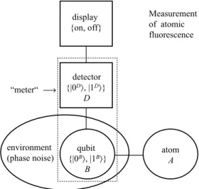
(9) G. Mack et al. / Physics Reports 540 (2014) 1–23. 9. Fig. 3. Scheme of measurement of atomic fluorescence.. environment which consists of the detected fluorescent field modes. The state of B gets entangled with the state of A – the atom – in a unitary evolution during τ , and the generalized measurement of A is completed by a von Neumann-type projective measurement on the entangled simulator B. As a consequence, the state of detector D (Fig. 3) mimics the state of B. However, the non-diagonal elements of ρB and ρD decay quickly by the coupling of B with the macroscopic detector, leaving the detector’s state diagonal,. ρD = p0 |0⟩⟨0| + p1 |1⟩⟨1|,. (35). where pi (i = 0, 1) is the probability for the respective states. We say that the detector clicks if it gets excited to the state |1⟩. If another photon is detected before the detector is reset to state |0⟩, this has no effect. But after some time, the detector is reset to |0⟩. Concerning the resetting. There are two possibilities: Reiterated attempts of recording separated by time increments τ may yield a random series of detector clicks to be registered by a display: The latter, initialized into its referential state ‘‘off’’, shifts to state ‘‘on’’ at time τ upon a photon detection at td where 0 ≤ td ≤ τ . This recording of the detector signal at time τ is made to set back the display to its state ‘‘off’’ with a small delay τm ≪ τ , and all fluorescence photons become consecutively registered. This procedure warrants a ‘‘selective’’ measurement of the atom’s fluorescence emission within the overall probing time T. In contrast, if the recording by the display is postponed to the end of the probe pulse, at time T, the display merely discriminates the final state ‘‘off’’: no photons, from ‘‘on’’: non-zero photons during the probe interval T. This is a ‘‘nonselective’’ measurement. 5.1. The system The model atom of Section 3, characterized by energy levels e and g, will be extended such as to include a metastable level s connected with the ground state g by a weak line, say, an electric quadrupole resonance (Fig. 4). The energy difference between e and g is denoted h̄ωeg , and the energy difference between s and g is h̄ωsg . The states |g ⟩, |e⟩ and |s⟩ span the 3-dimensional Hilbert space H A of states of the atom. In the preparatory first step, driving radiation of frequency ω′ = ωsg + ∆′ , detuned by ∆′ , is assumed to coherently interact with the atom for a time interval of length T ′ , lasting from time −T ′ to 0. This will prepare the atom in a definite state φ A (0). At the beginning of the preparation (‘‘driving’’), the atom is assumed to be in state |g ⟩. Then its state at time 0 is a superposition of |s⟩ and |g ⟩, and will be. φ A (0) = d0 |g ⟩ + d1 |s⟩. (36). where [33] d0 (0) = cos. θr′ 2. −i. ∆′ θ′ sin r , ′ Ωr 2. d1 (0) =. Ω′ θ′ ′ ′ sin r e−i∆ T . ′ Ωr 2. (37). Here is θr′ = Ωr′ T ′ , and Ωr′ is the generalized Rabi flopping frequency defined by.   2 Ωr′2 = ∆′ − i γs − γg + Ω ′ 2,. (38).

(10) 10. G. Mack et al. / Physics Reports 540 (2014) 1–23. Fig. 4. Driving and probing a three-level atom.. where Ω ′ is the Rabi frequency of the driving light. With the relaxation rates γs and γg being equal or neglected, and in the case of resonant driving (∆′ = 0),. θr′ = θ ′ = Ω ′ T ′ ,. (39). and d0 T ′ = cos.  . θ′ 2. ,. d1 T ′ = sin.  . θ′ 2. .. (40). In the second step, probing radiation which is nearly resonant with the transition g → e, of frequency ω = ωeg + ∆ is to act on the atom from t = 0 till t = T and excite resonance scattering. The resonant scattering occurs as a consequence of the coupling of the atom to a simulator B. The simulator B is the same as for two-level atom considered before, but the atom now has three states. For later discussion we distinguish bright states which are superpositions of |g ⟩ and |e⟩, and the dark state |s⟩. The driving prepares a superposition of the bright state |g ⟩ and the dark state |s⟩. By contrast, the probing only induces transition between bright states. 5.2. Coupling of system and meter The probe light induces a dipole moment on the line g − e of the atomic system whose interaction with the vacuum fluctuations of the spatial field modes generates fluorescent radiation. This field excitation heralding atomic decay to state g is the ancilla in the generalized measurement (POVM) on the atom: It is the target of the projective measurement by the detector. The fluorescent radiation is considered the only relaxation process of the free atom, generated by the radiative environment, and thus this measurement is performed on (part of) the environment of the atom. We suppose, for simplicity, that this environment is simulated by only one radiative mode, the simulator B. Let the creation and annihilation operators for this mode be denoted by aĎ and a. The measured observable is the energy h̄ωeg aĎ a of the fluorescent radiation. Since the atom may, out of state |e⟩, only emit one photon at a time, we restrict attention to states of the field with 0 or 1 photon. The configuration space of the field simulator B is then a two-dimensional Hilbert space H B spanned by the orthogonal eigenstates |0⟩ and |1⟩ of aĎ a. We define raising and lowering operators in H B as in (7), with |0(B) ⟩ = |0⟩, and |µ(B) ⟩ = |1⟩, and an interaction Hamiltonian HAB . The interaction HAB of atom A and simulator is the same as in the two-level atom, Eq. (25), and involves the product of the simulator’s Lindblad operator LBµ =. √ Bµ Γ σ−. (41). and a single atomic Lindblad operator L1 which describes the atomic decay. The time evolution of the atom A under the influence of the probe light, in secular approximation, is described by the time-independent Hamiltonian HA = HÂ + h̄ωse |s⟩⟨s|. (42). where HÂ is the Hamiltonian of the two-level atom, HÂ =. h̄∆r 2. σzA − ih̄. Ω 2. e−iϕ σ+A + ih̄. Ω 2. eiϕ σ−A ,. (43). with σz = |e⟩⟨e| − |g ⟩⟨g |, σ+A = |e⟩⟨g |, σ−A = |g ⟩⟨e|. The unitary time evolution UAB (t ) in H B ⊗ H A is UAB (t ) = exp(−i [HA + HAB ] t /h̄). It is followed by a projective measurement on B.. (44).

(11) G. Mack et al. / Physics Reports 540 (2014) 1–23. 11. Now suppose that the coupled system A + B is initially in state φ A (0) ⊗ |0⟩. The unitary time evolution during a short time interval τ maps this into the entangled state. |φ AB (τ )⟩ = (1 − iHA τ /h̄ − J τ )φ A (0) ⊗ |0B ⟩ +. √ τ L1 φ A (0) ⊗ |1B ⟩. (45). Ď. to first order in τ , with J = (1/2)L1 L1 . The excited state |1B ⟩ of the simulator models an emitted fluorescent photon. It decays quickly, at a rate Γ ≫ τ −1 , since its detection is destructive, and the detector is macroscopic. Thus, the simulator B is reset to |0B ⟩ early in the next time increment beginning at τ . 5.3. Detection and read-out The detector D performs a repeated projective measurements on the simulator B, such that the evolution of B after multiples of τ is stepwise mapped on that of the detector. Consequently, measurements of the quantum energy h̄ωa+ a of fluorescence are reduced to projections by the observable Pi = |iB ⟩⟨iB | at time τ , 2τ , 3τ . . . , and the state of D is conditionally described by the density matrix ρDi = Pi |φ A (τ )⟩⟨φ A (τ )|PiĎ /TrPi |φ A (τ )⟩⟨φ A (τ )|PiĎ . In measuring the atomic environment B, the detector D monitors the history of the atom: Random time intervals of undisturbed atomic evolution are interrupted by events of atomic decay that display jumps in the recorded trajectory of results. This causes phase diffusion of the Rabi nutation at the emission times of fluorescence photons, (see [26], Fig. 4.4). It can be shown that the non-diagonal elements of the density matrix ρ B of the simulator B decay quickly [28], and the diagonal elements are retained. In detail: The master equation of the atom’s environment turned into meter B is.   ρ̇ B = γ n̂ρ B n̂ − n̂2 ρ B /2 − ρ B n̂2 /2. (46). where n̂ = aĎ a is the number operator [28]. In the number basis, the matrix elements of the density operator evolve as.   γ ⟨n|ρ B (t )|m⟩ = exp − t (n − m)2 ⟨n|ρ B (0)|m⟩, 2. (47). such that the non-diagonal elements quickly decay, and the diagonal elements are retained. Thus, the atomic decay provides ‘‘pointer states’’ that represent the detector D, the measured state of B evades entanglement with the state of its own environment, and D qualifies as a ‘‘photon detector’’. Its actual state represents an ‘‘unread result’’ of the measurement on B, and we may drop the index D or B in the pointer states. Reading out the detector usually means to release a ‘‘click’’ with result |1⟩, and ‘‘no click’’ with result |0⟩. For a more general approach, let us assume that the results are to be read out by way of a macroscopic display with the reading ‘‘off’’ and ‘‘on’’ corresponding to results |0⟩ and |1⟩, respectively. The display is to read the result, and to reset the detector to its state |0⟩, after each time increment τ with a delay τd . If the reading is ‘‘on’’, there was an event of emission and detection during τ . Note that τd ≪ τ allows the faithful recording of all intervals with just one click and without a click, as long as the mean waiting time between the clicks, tw , far exceeds τ , i.e., tw ≫ τ . This mode of measurement is ‘‘selective’’. In contrast, when τd = T ≫ τ , and D starts off in the pointer state |0⟩ and switches to |1⟩ at a time k1 τ (k1 integer ), the detector is not reset up to the end of the probe pulse. This ‘‘non-selective’’ measurement only discriminates between results whose ‘‘off’’ on the display corresponds to ‘‘never |1⟩, and ‘‘on’’ to ‘‘not all |0⟩’’. We shall adopt this mode of detection in what follows. The probability of finding the eigenvalue 0 after the first time interval τ is Ď. p0 (0) = 1 − τ ⟨φ A (0)|L1 L1 |φ A (0)⟩,. (48). and the state of the atom is then projected to a new state. |φ A (τ )⟩ =. 1 − iHA τ /h̄ − J τ. √. p0 (0). |φ A (0)⟩.. (49). The factor p0 (0)−1/2 ensures that |φ A (τ )⟩ has norm 1. The state |φ A (τ )⟩ is made to evolve during the next time interval in order to come up with |φ A (2τ )⟩, and so on. It follows that the conditional probability after kτ given that no click occurred in the preceding time intervals the pointer state is still |0⟩, and the display still shows ‘‘off’’ is Ď. p0 (kτ ) = 1 − τ ⟨φ A (kτ )|L1 L1 |φ A (kτ )⟩,. (50). and the state of the atom will then be. |φ A ((k + 1)τ )⟩ =. 1 − iHA τ /h̄ − J τ. √. p0 (kτ ). |φ A (kτ )⟩.. (51).

(12) 12. G. Mack et al. / Physics Reports 540 (2014) 1–23. If the pointer state is |0⟩, and the display shows ‘‘off’’ at some time t = kτ between 0 and T then we know that pointer state |1⟩ has never been observed (no click has occurred) at any time increment before t. It follows (by iterating Eq. (51)) that the state of atom at time t is 1. |φ A (t )⟩ = √. Nt. exp (−i[HA /h̄ − iJ ]t )|φ A (0)⟩,. (52). where Nt is the probability that the pointer state at time t has never been |1⟩, and the display still shows ‘‘off’’. It can be determined from the requirement that this state is normalized. The initial state of the atom at time t = 0 was prepared to be. |φ A (0)⟩ = d0 |g ⟩ + d1 |s⟩.. (53). It follows that 1. |φ A (t )⟩ = √. . Nt. d0 exp (−i[HA /h̄ − iJ ]t ) |g ⟩ + d1 e−iωsg t |s⟩ .. . (54). The norm of this state is Nt = d20 exp (−γe t ) + d21 .. (55). In case that level s cannot be approximated as being stable, the last term has to be completed by the factor exp(−γs t ). Under experimental conditions of interest, γe ≫ T −1 ≫ γs . Therefore, up to an exponentially small error, the atom is in the state. |φ A (T )⟩ = e−iωsg t |s⟩. (56). if the display at time T shows ‘‘off’’, indicating that no fluorescent photon was recorded at any time before T, and the probability for this is NT = |d1 |2 .. (57). Recall that |s⟩ is the ‘‘dark state’’ of the atom, and all the states in the two-dimensional Hilbert space spanned by |g ⟩ and |e⟩ are ‘‘bright states’’. Mixtures of bright states are also called ‘‘bright states’’. This terminology is motivated by the atom’s dark state being correlated with pointer state |0⟩ and display reading ‘‘off’’, while the bright states, or their superpositions or mixtures, are correlated with pointer state |1⟩ and display reading ‘‘on’’ such that at least one photon was detected during the probe interval T. We will now argue that at least one fluorescent photon will be detected during the probe interval of length T if the atom is initially in the bright state |g ⟩, while none is detected if the atom is initially in the dark state |s⟩. This assertion assumes that the probe interval is very long compared to τ . The assertion is deduced from the quantum regression theorem which confirms that the probability of resonance fluorescence is equal to the probability that the atom is in the excited state |e⟩. This probability is equal to the expectation value 21 (⟨σz ⟩ + 1). It is determined by solution of the Lindblad equation for atom + simulator. The result can be deduced from the known result for a two-level system [28, Eq. (10.59)]:. ⟨σ+ (t )σ− (t )⟩ = =. 1 2. (⟨σz ⟩ + 1) Ω2. (γe /2)2 + 2Ω 2. . 1 − e−3γe t /4. . cosh κ t +. 3γe 4κ. sinh κ t.  (58). where. κ=. 1. . (59) (γe /2)2 − (4Ω )2 , 2 σ+ , σ− , σz are the components of the atomic spin vector, and Ω is the Rabi frequency of the probe radiation at the atom’s site. If Ω is below γe /8, the probability approaches a stationary state, otherwise it oscillates. In any case, resonance fluorescence will occur in a sufficiently long time interval T. Thus, the conditional probability for a scattering event at time t after the start of the probe pulse is d20 (T ′ )⟨σ+ σ− (t )⟩. Upon arrival of the first photon, the pointer state switches from |0⟩ to |1⟩, which is kept as an ‘‘unread’’ result, when the display is supposed to operate in the delayed mode that resets the detector eventually at the end of the probe pulse, at time T. Consequently, each probe pulse having caused the detection of at least one photon is correlated with the meter’s pointer state ‘‘on’’. The probability that the atom is in a bright state at the end of the drive–probe interaction, when the initial state at time −T ′ was the bright state |g ⟩, and the probability that the atom is in the dark state at the end when the initial state is the dark state |s⟩, are equal and given by the initial probabilities of bright vs dark states, Eqs. (37) and (40), as P (bright → bright) = p11 = cos2. θ′ 2. = p00 = P (dark → dark).. (60).

(13) G. Mack et al. / Physics Reports 540 (2014) 1–23. 13. In conclusion, probing with delayed readout performs a measurement of whether the atom has or has never decayed from its excited state |e⟩ to its ground state during the probing interval of duration T. If state |s⟩ is long-lived, i.e. if γe ≫ γs holds, an ‘‘off’’ result on the display indicates survival of the atom in the dark state |s⟩, while an ‘‘on’’ result signals the appearance of an undisclosed number of transitions to the bright states. For an alternative verification of these statements, suppose that at time T the pointer state is |1⟩ and the display shows ‘‘on’’. Then there must have been at least one (unread) click of the detector. Suppose it occurred at time t. Right after the click, the atom is in state |g ⟩. Later clicks have no effect on the pointer states. Therefore the state of the atom evolves under the unitary time evolution of atom + detector for time intervals τ , followed by unread measurements of PB = |1⟩⟨1|. In general, this leads to a mixed state, which is described by a density matrix ρA (t ′ ), t ′ ≥ t. Enumerating the states |s⟩, |g ⟩, |e⟩, by 0, 1, 2, a bright state will have a density matrix of the form. ρA (t ′ ) =. . . 0 0. 0 ρ̂A (t ′ ). (61). where ρ̂A is a density matrix for the two level atom with pure states |g ⟩, |e⟩. The initial state |g ⟩ at time t corresponds to a density matrix ρA (t ) = |g ⟩⟨g |. This is a projector. It is to be shown that the time evolution is such that the density matrix is of the same form ever thereafter. According to the general theory, the time evolution is described by the Lindblad equation, dρA (t ) dt. =. −i h̄. Ď. [HA , ρA ] + L1 ρA L1 −. 1 2. Ď. L1 L1 ρA −. 1 2. ρA LĎ1 L1 .. (62). If ρA is of the form of a projector, then all the terms on the right hand side of this equation are of the same form and so is therefore dρ/dt. The form of the density matrix of a bright state of the atom is therefore perpetuated, as claimed. 5.4. Successive cycles of measurement The strategy of measurement outlined above that makes use of final readout and reset only seems to entail an enormous waste of recordable information, namely of the arrival times of individual detector clicks, and saving only one result per measurement cycle. This mode of detection leaves a potentially selective measurement merely non-selective. However, single-photon detection of an atom’s resonance fluorescence requires temporal resolution in the sub-nanosecond range. It is afflicted by much less than perfect efficiency, in particular with a detector whose spatial angle of acceptance covers a small fraction of 4π only. In contrast the above type of measurement warrants close to 100% efficiency thanks to the large number of fluorescence photons detected within T. In order to provide access to a selective mode of detection, an ensemble of subsequent drive–probe interactions has to be applied to the atomic system. This approach is applicable as long as the duration of an individual drive–probe cycle does not exceed the lifetime of level s, i.e. T ′ + T < γs−1 .. (63). Consider now a sequence of drive–probe cycles applied on the atom with recording of the terminal pointer state of each cycle. From the result of the previous subsection, the probabilities of sequences of q equal results (‘‘on’’ or ‘‘off’’) may be calculated. We compute the conditional probabilities P (on/off|r ) for results ‘‘on’’ and ‘‘off’’ in the (n + 1)st experiment, given that the result of the previous experiment was r, where r = ‘‘on’’ or ‘‘off’’. A very short time after the end of the probe pulse of the nth cycle, the state of the atom is |g ⟩ if r = ‘‘on’’, and |s⟩ if r = ‘‘off’’. The result (60) together with Eqs. (40) imply that the conditional probabilities are P (off|off) = cos2 P (on|off) = sin2. θ′ 2. θ′ 2. ,. (64). ,. (65). independent of n, and P (on|r ) = 1 − P (off|r ). Therefore, P (on|on) = P (off|off) ,. P (on|off) = P (off|on) .. (66). The probability Pq (r ) that the detection of a pointer state r at the end of the nth drive–probe cycle will be followed by at least q − 1 detections of the same pointer state r in the q − 1 following drive–probe cycles, is therefore Pq (r ) = cos2(q−1). θ′ 2. ,. (67). independent of r and n. These results can be used to reestablish a selective measurement using a sequence of pump–probe cycles, and to exemplify the QZE..

(14) 14. G. Mack et al. / Physics Reports 540 (2014) 1–23. 6. The quantum Zeno effect The QZE is a prediction of quantum theory which asserts that frequent observation inhibits or retards the evolution of an unstable quantum system ([9]–[11], see also [34]). The experimental verification of the QZE can furnish insight concerning the foundations of quantum theory, including measurement theory. Potential insight presupposes that the requirements are precisely specified which must be fulfilled in order that such a non-trivial inhibition may take place. The QZE as defined originally by Misra and Sudarshan [11] requires entanglement of system and meter in the course of observations, which are in fact measurements (or ‘‘monitoring’’) of the survival of the unstable system in its initial state. It is obvious that a measurement of survival of the system must be performed on an individual system, not on an ensemble of systems: 1. Measurements of the residual of the systems in the (large) ensemble left over in their initial state yield relaxation rates γ = Σ (1/Tn ), where Tn is the survival time of the nth system. Being average values already, these rates do not represent the results of quantum measurements, namely eigenvalues. Several experiments which have been claimed to demonstrate QZE – including the experiment on a cloud of trapped ions by Itano et al. [13] – were based on the recording of relaxation rates and could not acquire survival times, let alone from quantum measurements [35]. For the demonstration of the QZE, the acquisition of survival times by observations on an individual quantum object, as in the experiments by Balzer et al. and Toschek et al. [18–20] are indispensable. Also, measurements of the survival time on an individual system by a series of interactions whose individual results are left unrecorded – except the result of the final interaction – do not prove QZE: 2. Again, the result of the final monitoring represents an average value, not an eigenvalue. Moreover, the final monitoring cannot warrant survival of the system in its initial state: It may have been in different eigenstates at intermediate times, since trajectories including back-and-forth transitions are not rejected [16]. This fact has been addressed as ‘‘repopulation effect’’ [36]. Restriction of the measurements to read-out after the final interaction only, i.e., to non-selectivity, as in the experiment of Itano et al. [13] does not provide knowledge of the micro-structure of the ensemble of measurements, that contains statistical information on the survival times. In contrast, results of all the intermediate measurements were read out with the experiments of Refs. [18–20]. The decrease of a relaxation rate (1) as well as the less decreased population of the initial state found by mere final recording of the state population (2) both occur with the true QZE, but also with interactions that may be described by rate equations, as the saturation of an atomic line by quasi-monochromatic light [37]. Consequently, the observation of each of these phenomena provides a necessary, but not a sufficient condition for the presence of a QZE. Thus, the proof of QZE demands a sequence of recordings on an individual quantum object [38] with read-out results (‘‘selective’’ measurements) for survival times: 3. These results are eigenvalues. They are conditionally random and allow the determination of the (mean) survival time. The procedure amounts to a genuine quantum measurement that conveys information on an observable of the system, available in the trajectory of the results. The QZE as defined originally [11] requires entanglement of system and meter in the course of a quantum measurement of survival of the system. Home and Whitaker [17] have noticed that dynamical interaction of system and meter might cause a more trivial situation which does not need, for explanation of the system’s enhanced survival, to recur to an effect of observation. Consequently, effects based on dynamical interaction – which indeed are fairly ubiquitous [36] – should not be considered to demonstrate the true QZE. The presence of such dynamical effects cannot be excluded in many attempts for demonstration of the QZE—except when the observations are based on QND measurements. We follow Home and Whitaker [17] who have suggested to restrict the attribute of genuine QZE, or QZP, to the inhibiting effect emerging from reactionless interaction of system and meter, although collecting information on the system. Typical manipulations of this kind are known as quantum non-demolition (QND) measurements [39], in particular measurements with a null result. Experiments that comply with all the above requirements have been performed on individual trapped ions, probed by light pulses [18–20], and recently on individual photons, probed by atoms [40]. The prototypical example of the QZE in a material system is the decay of the excited state of a two-level atom (equivalent to a spin) which is exposed to resonant radiation, and efficient photon counting of the resonance fluorescence. Such a test of the spontaneous decay of a system would require extremely high temporal resolution of the photon detection and typically suffers from low detection efficiency. The drive–probe experiments considered here are less demanding. It is assumed that the drive light stimulates transitions between the bright state |g ⟩ and the dark state |s⟩ of the atom, and the application of the probe light combined with reading a pointer effects a measurement of whether the atom is in a bright state or in a dark state at the end of the drive pulse. Consider a sequence of N drive–probe cycles of total duration T0′ = NT ′ of the drive pulses. All the drive pulses have the same pulse area θ ′ . We assume that the g − s line is dipole-forbidden. It suffices to consider the case of resonant radiation (∆′ = 0), so that. θ ′ = Ω ′T ′ =. Ω ′ T0′ N. .. (68). The total duration T0′ is considered fix so that the pulse area is proportional to 1/N. Now consider the probability that, starting from the bright (dark) state |g ⟩ at time −T ′ , all the N measurements yield the result ‘‘on’’ (‘‘off’’), i.e., the atom keeps.

(15) G. Mack et al. / Physics Reports 540 (2014) 1–23. 15. Fig. 5. Scheme of measurement of atomic absorption.. staying in its state up to the final detection. Correlated with the orthogonal states a|g ⟩ + b|e⟩ = |on⟩ and |s⟩ = |off⟩ are the orthogonal pointer states |bright⟩ and |dark⟩, respectively [41]. Then, according to Eqs. (60) and (68), the probability for such a homogeneous outcome is P (all on|bright) =. . cos2. Ω ′ T0′ 2N.  ≈ exp −. 1 4N. N. = P (all off|dark). (Ω T0 ). ′ ′ 2. (69).  −−−→ 1 N →∞. (70). in the limit of large N, i.e. of frequent measurements. This may be contrasted with the probability when intermediate measurements are lacking. It can be deduced from Eqs. (37)–(40) that this probability equals P (bright|bright) = cos2. Ω ′ T0′ 2. = P (dark|dark).. (71). This is seen as follows: The action of the probe pulses leaves bright states of the atom bright and dark states dark. If at the end of a probe pulse, the state is bright, it turns into |g ⟩ very quickly, (emitting a fluorescent photon if it is |e⟩). Therefore we may regard the state to be a superposition of |g ⟩ and |s⟩ at the beginning of the next drive pulse. Therefore the effect of the N drive pulses adds up as if the probe pulses had not taken place. In the above scenario, the measurements have suppressed the time evolution induced by the drive pulses. In fact, with probability very close to 1, all the measurements give the result that the atom stayed in a dark (bright) state if the initial state was dark (bright). Such drive–probe experiments are quantum non-demolition experiments. This is exactly true for the measurement of P (all off | dark), and true in very good approximation in case of the measurement of P (all on | bright). 7. The emergence of pointer states: absorptive probing So far we have analyzed the atom being probed by the detection of its resonance fluorescence, which is part of the atom’s interaction with its environment, the general radiation field. Since the meter signal – the scattering rate in the field modes recorded by the detector – represents the reaction of the environment, the meter states ‘‘on’’ and ‘‘off’’ are natural ‘‘pointer states’’ of the environment turned into a meter. In general, these states are defined as eigenstates of a pointer observable that commutes with the interaction Hamiltonian of atom and environment. The pointer states are supposed to emerge in the course of the evolution of the entangled system and meter under the action of the environment [25,28]. A demonstration of this emergence requires the application of a meter not being identified with (part of) the environment. Such a suitable approach being alternative to a measurement on the atom via its resonant light scattering is the recording of the absorptive or dispersive effect imposed upon the exciting light field by the atom. Such a scheme features a channel of detection separate from the modes of the environment although influenced by the environment via the atom (Fig. 5). Here, we shall outline the evolution of pointer states in this more general kind of measurement. As in the above model, a three-level atom is assumed irradiated by subsequent pulses of drive and probe light. In this open system, the coherent field mode of Fig. 5 is represented by a single-mode light beam of amplitude E . We restrict attention to the absorptive interaction with the atom. The atomic excitation |g ⟩ → |e⟩ is accompanied by the loss of a photon from the field E , that is recorded [42,43]. Since we want to distinguish two states of the atom, ‘‘on’’ and ‘‘off’’, two states of the.

(16) 16. G. Mack et al. / Physics Reports 540 (2014) 1–23. Fig. 6. Environment-generated evolution of pointer states in the measurement of atomic absorption (from Ref. [44]). ΩR /γ = 0.6 (line 1), 2 (line 2), 5 (line 3).. meter – now the light flux of the probe beam – suffice for a full characterization of the meter. For this purpose, we introduce a ‘‘meter simulator’’ with states {|0D ⟩, |1D ⟩} corresponding to flux levels I0 , I, with atomic absorption absent and present, respectively. The entire system is modeled by the density matrix of the atom immersed in the environmental field, extended by the meter simulator, a so-called ‘‘purification’’ of ρA. |ΦAD ⟩ =. 1  √. pj |ΦjA ⟩ ⊗ |ΦjD ⟩. (72). j =0. . i pi = 1. The operation UM [26, Eq. (4.28)] entangles atom and meter simulator,   D ρ̂(t ) = UM (t ) ρ̂A (0) ⊗ |u0 ⟩⟨uD0 | UMĎ (t ). with the probabilities obeying. =. 1 . Mi ρ A Mj ⊗ |uDi ⟩⟨uDi |,. (73). i,j=0. where |0D ⟩ is a reference state of the meter, and Mi are Kraus operators that define a generalized measurement (POVM) on the atom. Explicitly, the entangled state is. ρ̂(t ) = M0 ρ̂A M0Ď ⊗ |0D ⟩⟨0D | + M0 ρ̂A M1Ď ⊗ |0D ⟩⟨1D | + M1 ρ̂A M0Ď ⊗ |1D ⟩⟨0D | + M1 ρ̂A M1Ď ⊗ |1D ⟩⟨1D |. (74). where ρ̂A = ρ̂ (t ) is to describe the dynamics of the atomic system interacting with the light field and environment. This dynamics is derived from the master equation [26, Eqs. (4.71), (3.147)], A. dρA. = −i.  γe ωge  σz − dge E , ρA − (σ+ σ− ρA + ρA σ+ σ− − 2σ− ρA σ+ ). (75) 2 2 where σz is the z-component of the spin operator with eigenstates |g ⟩ and |e⟩, dge the atomic dipole moment, and the decay constant γe of the atomic resonant state characterizes the coupling to the environmental field. Absorption of a photon by the ground-state atom requires M1 to be identified with the atomic raising operator σ+ = 21 (σx + σy ) = |g ⟩⟨e|, while the residue in the ground state is met by the projector M0 = |g ⟩⟨g |. From an analytic solution of the atomic density matrix [44, Eqs. (10.52) and (10.54)], we have dt. A ρee (t ) =. ΩR2. . 2(ΩR2 + 2γe2 ). 1+. λ2 λ1 eλ1 t + eλ2 t λ1 − λ2 λ2 − λ1.  (76). where in case of pure radiative damping 3. . λ1,2 = − γ ± 2. 1 4. γ 2 − ΩR2. (77). with γ = γe /2. Fig. 6 shows the evolution of the occupation probability of the resonance level |e⟩. Note that this probability approaches an asymptotic steady state that monotonically increases with the flux of the light beam. The probe beam is to be detected by photon counting. The light flux J (counts per time unit) allows I0 = J /γe counts within the lifetime of the resonance level. The atomic absorption reduces this mean counting rate by the rate of fluorescence, which is proportional to the atomic density in the excited state, A I (t ) = I0 − γe ρee .. (78).