Full PDF

Texto completo

(1)Diversity and distribution of Odonata (Insecta) larvae along an altitudinal gradient in Coalcomán mountains, Michoacán, Mexico José Antonio Gómez-Anaya1, Rodolfo Novelo-Gutiérrez1 & William Bruce Campbell2 1. 2.. Instituto de Ecología, A.C., Carretera Antigua a Coatepec 351, El Haya, 91070, Xalapa, Veracruz, Mexico; [email protected], [email protected] Cardno ENTRIX, 701 University Avenue, Suite 200, Sacramento, California, 95825, USA; [email protected] Received 13-IX-2010.. Corrected 12-II-2011.. Accepted 16-III-2011.. Abstract: Evaluating components of landscape diversity is essential for the implementation of efficient conservation strategies. We evaluated the diversity of Odonata larval assemblages from the Coalcomán mountains (CM), Michoacán, Mexico, and related it to local (site-level) habitat variables. Larvae were collected from shores, riffles and pools in five streams, counted and identified to species, twice per season during 2005. The Shannon Diversity Index (H’), Margalef’s Richness Index (R), Simpson’s Index as a dominance measure (D) and Pielou’s Equitability (J) were used to describe the assemblages, and Renyi’s Diversity Profiles were used to order diversity. A Bray-Curtis Similarity Index (BC) was used to evaluate beta diversity. Theoretical richness was estimated using non-parametric and parametric methods. A Canonical Correspondence Analysis (CCA) was applied to explore the relationships of species with site-level environmental variables. A total of 12 245 larvae from 75 species, 28 genera and 8 families were recorded. Over all sites, the dominant species were Erpetogomphus elaps, Macrothemis pseudimitans and Argia pulla. The number of species per locality ranged from 18 to 36, and a high number of species (76%) occurred with relative abundances lower than 1%. A differential distribution of species and abundance in streams, time and strata was observed. Renyi’s diversity profiles showed diversity was higher in spring and on shores. Most BC similarity values were smaller than 25%, indicating a high turnover rate in the CM. The high turnover rate reflects a differential distribution of the species along the altitudinal gradient, supporting the hypothesis of Mexico as a betadiverse country. According to the slope of Clench’s curve, a reliable list of species was gathered. The CM larval assemblage is currently the largest reported for Mexico, and our results support previous proposals of the CM as a species-rich area for conservation. Rev. Biol. Trop. 59 (4): 1559-1577. Epub 2011 December 01. Key words: dragonfly larvae, diversity, CCA, Coalcomán Range, Michoacán, Mexico.. Given its topography, climatic diversity and geographical situation between two biogeographic regions (Neotropical and Nearctic), Mexico is a megadiverse country (Mittermeier et al. 1998). It is well known that the rate of species lost worldwide (Fraser et al. 1993) surpasses that by which taxonomic knowledge is increased. Thus, it is necessary to intensify studies focusing on diversity and from areas with an acceptable level of conservation. Presently, there are many taxonomic studies on larvae and imagoes of Mexican Odonata,. but the ecological studies are relatively scarce, especially for short and long term evaluations on possible changes induced by human activities (e.g. climatic change). Additionally, ecological studies on richness and distribution at regional levels are few. It is well known that Odonata larvae are dependent on habitat characteristics (Watson et al. 1982), sensitive to abiotic factors, and play significant roles as predators and prey in the trophic structure of aquatic communities (Corbet 1999). They possess many desirable bioindicator qualities. Rev. Biol. Trop. (Int. J. Trop. Biol. ISSN-0034-7744) Vol. 59 (4): 1559-1577, December 2011. 1559.

(2) (Carle 1979, Samways 1993, Clark & Samways 1996, Moore 1997, McGeoch 1998, Corbet 1999, Chovanec & Waringer 2001, D’Amico et al. 2004), and many species have been used to study a variety of phenomena, such as tolerance to physicochemical factors (Carchini & Rota 1985, Ferreras-Romero 1988, Rodríguez 2003, Remsburg et al. 2008), accumulation of metals in larvae (Gupta 1995), effects of increased water temperature caused by nuclear reactors (Gentry et al. 1975, Thorp & Diggins 1982), direct sewage discharge to rivers (Watson et al. 1982), pesticide contamination (Takamura et al. 1991, Hurtado-González et al. 2001), impact from cattle ranching on imago assemblages (Hornung & Rice 2003, Foote & Hornung 2005), relationships of assemblages with habitat characteristics (Castella 1987, Bulánková 1997), and larvae as indicators of water quality (Trevino 1997), total richness (Sahlén & Ekestubbe 2001), and riparian quality (Smith et al. 2007). Several studies also have focused on their application in diversity and conservation assessment (Hawking & New 2002, Clausnitzer 2003, Bried et al. 2007, Campbell & Novelo-Gutiérrez 2007, Campbell et al. 2010). The objective of this study was to assess the variation of diversity in Odonata larval assemblages along an elevation gradient and their relation with stream habitat variables by season and habitat. Local and landscape information on assemblage diversity may be useful in supporting conservation efforts and in following short and long term changes in their diversity in the Coalcomán Mountains. MATERIALS AND METHODS Study area: The Coalcomán Mountain Range (CM) in Michoacán, Mexico, is located between 18° 35’40”-19°00’31” N and 102°27’47”-103°40’36” W. The climate is predominantly tropical (annual average temperature 26.5°C), with a rainy period occurring in summer, and average annual precipitation ranging from 700mm in the lowlands to 1 300mm in the highlands (Antaramián 2005). The CM 1560. is one of the least disturbed regions in Michoacán. The studied assemblages are located in streams within Hydrological Priority Region 26 (Río Coalcomán and Río Nexpa; Arriaga et al. 1998), and Terrestrial Priority Region 115 (Sierra de Coalcomán; Arriaga et al. 2000) in Michoacán State, Mexico. The sampled streams included Ticuiz (TZ), Estanzuela (EZ), Río Pinolapa (RP), Colorín (CL) and Chichihua (CH). Details on water channels and averages of physicochemical data for the streams have been published by Novelo-Gutiérrez & GómezAnaya (2009), and are summarized in Table 1. Larval collection and physicochemical measures: Larval sampling was conducted twice per season during 2005, as follows: February 17-21(winter); March 29-April 2 and May 31-June 4 (spring); July 6-10 and August 17-21 (summer); September 28-October 2 and November 8-12 (autumm) and January 18-22 (2006, winter). Larvae were collected during one day per stream, along a 500m stream segment using a D-frame aquatic net (0.2mm mesh). A stratified random sampling design was applied for stream margins, riffles and pools. A total of 12 samples were taken each time (3 samples in riffles, 3 samples in pools and the remaining 6 samples along margins). All samples were preserved in 96% ethanol with a replacement before 24h had elapsed. Odonata larvae were separated from the other fauna and stream debris using a stereomicroscope, counted and identified to species. All specimens were deposited in the Instituto de Ecología, A.C., Entomological Collection (IEXA). Physicochemical data (pH, temperature, dissolved oxygen, and conductivity) were recorded during each trip using a digital water analyzer (ICM Model 51500, Industrial Chemical Measurement, Hillsboro, Oregon, USA). Stream width, depth and current velocity were measured using a metric power tape and a digital flow meter (Global Water Flow Probe, Forestry Suppliers, Jackson, Mississippi, USA). At each point where we measured the stream’s width, several measures of water depth and velocity were taken and averaged to calculate discharge as: width x average depth x average. Rev. Biol. Trop. (Int. J. Trop. Biol. ISSN-0034-7744) Vol. 59 (4): 1559-1577, December 2011.

(3) TABLE 1 Annual means and ranges (Min – Max) for the stream physicochemical variables Stream/variable Elevation (m asl) Depth (m) Min - Max Width (m) Min - Max Velocity (m/s) Min - Max Discharge (m3/s) Min - Max N Temperature (ºC) CI 95% pH CI 95% Conductivity (µ/cm) CI 95% O2 (ppm) CI 95% N Gradient (slope) Min Max N. TZ 10 0.21 (0.13 - 0.38) 4.5 (0.4 -11) 11.08 (0.22 -32.7) 11.06 (0.05 - 35.9) 15 29.35 (28.42 -30.27) 7.47 (7.35 - 7.6) 640.5 (616.6 - 664.3) 4.31 (3.65 - 4.98) 36 1º 8’ 44.75’’ 0º 27’ 30.08’’ 2º 24’ 18.03’’ 7. EZ 408 0.1 (0.07 - 0.16) 1.67 (0.25 - 2.35) 0.49 (0.22 - 1.23) 0.05 (0.03 -0.08) 6 26.48 (25.56 -27.4) 8.08 (7.95 - 8.21) 509.83 (485.9 - 533.7) 7.53 (6.87 - 8.2) 36 4º 44’ 40.83’’ 1º 8’ 44.75’’ 6º 37’ 0.26’’ 7. RP 616 0.11 (0.04 -0.34) 2.18 (0.4 - 6.1) 0.38 (0.22 - 0.56) 0.09 (0.01 - 0.46) 8 28.03 (27.02 - 29.04) 8.47 (8.33 - 8.61) 666.83 (640.7 - 692.9) 7.78 (7.05 - 8.51) 30 1º 8’ 44.75’’ 0º 20’ 37.57’’ 2º 24’ 18.03’’ 7. CL 1050 0.14 (0.04 - 0.27) 1.85 (0.45 - 4.27) 6.57 (0.22 - 26.1) 1.66 (0.01 - 7.52) 10 20.14 (19.29 - 21) 7.54 (7.42 - 7.66) 50.08 (28 - 72.2) 8.37 (7.75 - 8.98) 42 7º 48’ 3.45’’ 1º 1’ 52.37’’ 15º 19’ 22.69’’ 7. CH 1130 0.12 (0.04 - 0.26) 3.23 (0.2 - 7.22) 6.87 (0.22 - 26.8) 2.4 (0 - 11.5) 15 22.62 (21.69 - 23.54) 8.16 (8.04 - 8.29) 460.89 (437 - 484.7) 7.74 (7.08 - 8.41) 36 1º 49’ 58.22’’ 0º 48’ 7.52’’ 4º 34’ 26.12’’ 7. CI=Confidence Interval, TZ=Ticuiz, EZ=Estanzuela, RP=Pinolapa, CL=Colorín, CH=Chichihua (modified from NoveloGutiérrez & Gómez-Anaya 2009).. current velocity. Finally, gradient was calculated according to Resh et al. (1996). For data analysis a one-way analysis of variance (ANOVA) was used to analyze the effect of stream on gradient, and a two-way multivariate analysis of variance (MANOVA) was applied to analyze the effect of stream and season on physicochemical variables. If significant effects were detected, we performed multiple comparisons using the Bonferroni t-test. All tests were performed using STATISTICA (StatSoft 2006). Diversity indices: Richness and composition, Shannon Diversity Index (H’), Margalef’s Richness Index (R), Simpson’s Diversity Index as a dominance measure (D), and Pielou’s. Equitability (J) (Moreno 2001) were used to describe the assemblages. To compare the diversity of the streams, Renyi’s profiles were generated (Tóthmérész 1995, 1998, Southwood & Henderson 2000, Jakab et al. 2002) because they include the logarithm of species number, H’, D, and the logarithm of Berger-Parker diversity (Tóthmérész 1995). The profiles also have a scale parameter (α) such that when the value of the parameter is low, the method is extremely sensitive to the presence of rare species, but as the value of the parameter increases, the profile becomes less sensitive. As a large scale parameter, the method is sensitive only to the more frequent species. The result of this scale-dependent characterization of diversity can be presented in graphic form. Rev. Biol. Trop. (Int. J. Trop. Biol. ISSN-0034-7744) Vol. 59 (4): 1559-1577, December 2011. 1561.

(4) to visualize relationships among communities: the community’s diversity profile’. If the curves of two diversity profiles intersect, then one of the communities is more diverse for rare species, while the other is more diverse for frequent species. Gamma richness estimation: An estimation of the theoretical richness using nonparametric methods (presence/absence: Chao2, Jack2, Bootstrap; abundance: ACE, Chao1) was carried out using EstimateS 8.0 (Colwell 2006). Additionally, parametric methods (richness estimators that use the observed species accumulation curve for modeling the addition of new species by extrapolation in relation to sampling effort) also were applied (Palmer 1990, Soberón & Llorente 1993), and included Clench’s (Clench 1979) and Linear Dependence (von Bertalanffy 1938) models, as well as the slope of the cumulative species curve to assess the completeness of assemblages (Jiménez-Valverde & Hortal 2003, Hortal & Lobo 2005). Slopes were obtained by means of the first derivative of Clench’s and Linear Dependence functions (Novelo-Gutiérrez & Gómez-Anaya 2009). Classification and ordination: Cluster Analysis (CA) on a Bray-Curtis (BC) similarity matrix with unpaired group mean average (UPGMA) amalgamation was used to explore faunal similarities among streams and seasons. This analysis was performed using PC-ORD v4.5 (McCune & Grace 2002). Additionally, a Canonical Correspondence Analysis (CCA) (CANOCO for Windows v4.5) was used to relate transformed species abundance [log(y+1)] to environmental variables (ter Braak 1986). The number of environmental variables was then reduced using the automatic forward selection option in CANOCO. Variables explaining most of the variation in the data were used to construct the final model. The statistical significance of the relationship between species and environmental variables was tested using a Monte Carlo permutation test (n=499), with an F-ratio as the sum of all 1562. eigenvalues for the test statistic (ter Braak & Prentice 1988, ter Braak & Smilauer 2002). RESULTS Physicochemical variables: Streams had significantly different gradients (slopes) (oneway ANOVA: F4, 30=10.17, p<0.01), and the Bonferroni paired t-test with multiple comparisons indicated that CL (Colorín) had the highest slope while RP (Pinolapa) and TZ (Ticuiz) had the lowest (Table 1). There was a significant difference among streams (one-way MANOVA: Wilk’s lambda=0.46, F16, 141=2.53, p<0.05) for width, depth, current velocity and discharge. The Bonferroni paired t-tests showed differences in depth and discharge for TZ with CH (Chichihua), EZ (Estanzuela) and RP. There was a significant difference in width between TZ and CL, while significant differences in current velocity were observed for TZ with EZ and RP. A two-way MANOVA showed a significant effect of stream (F16, 480.3=228.8, p<0.05), seasons (F12, 415.7 =182.2, p<0.05) and their interaction (F48, 606.8=17.6, p<0.05) on physicochemical variables. A Bonferroni paired t-test showed significant differences (p<0.05) in temperature among streams, except that of RP to EZ and TZ. Sites CL and CH exhibited the lowest average temperatures, 20.14ºC and 22.62ºC, respectively, while the highest were those of TZ (29.35 ºC) and RP (28.03ºC). Most of the Bonferroni contrasts were significant for pH, except those between CH-EZ and CL-TZ, and all sampling sites had a basic pH. The Bonferroni contrasts for temperature among seasons showed significant differences between autumn-spring, autumn-summer and springsummer. The average winter temperature was lower than that for the other seasons (Table 2). Most of the paired comparisons for conductivity showed significant differences among sites (p<0.05), except those between EZ and CH, and between RP and TZ. CL exhibited the lowest average value of all streams (50.08µ/cm). There was no significant difference in conductivity among seasons (p>0.05). The Bonferroni. Rev. Biol. Trop. (Int. J. Trop. Biol. ISSN-0034-7744) Vol. 59 (4): 1559-1577, December 2011.

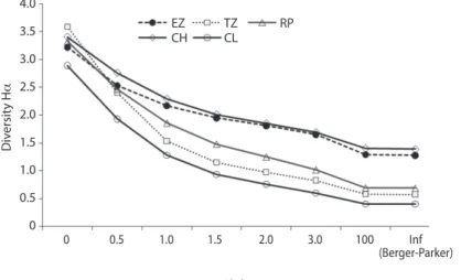
(5) TABLE 2 Means ± 95% confidence interval for physicochemical variables by stream and season (n=12) Stream. Season. Temperature (°C). CI 95%. pH. CI 95%. Conductivity (µ/cm). CI 95%. RP RP RP RP CH CH CH CH CL CL CL CL EZ EZ EZ EZ TZ TZ TZ TZ. Winter Autum Spring Summer Winter Autumn Spring Summer Winter Autumn Spring Summer Winter Autumn Spring Summer Winter Autumn Spring Summer. 20.93 26.18 31.90 34.95 17.47 22.77 23.43 25.85 16.55 21.45 19.42 21.36 21.37 26.73 28.53 27.76 25.40 30.39 30.22 29.84. ±0.61 ±0.43 ±0.61 ±0.61 ±0.61 ±0.43 ±0.44 ±0.61 ±0.61 ±0.43 ±0.43 ±0.43 ±0.61 ±0.43 ±0.61 ±0.43 ±0.61 ±0.43 ±0.61 ±0.43. 8.50 8.11 8.68 8.95 7.80 8.16 8.14 8.58 7.00 7.27 7.51 8.11 7.70 7.96 8.02 8.42 7.50 7.27 7.47 7.67. ±0.13 ±0.09 ±0.13 ±0.13 ±0.13 ±0.09 ±0.09 ±0.13 ±0.13 ±0.09 ±0.09 ±0.09 ±0.13 ±0.09 ±0.13 ±0.09 ±0.13 ±0.09 ±0.13 ±0.09. 740.17 567.83 706.33 752.00 460.82 440.83 478.50 465.83 105.50 31.31 45.13 46.10 462.13 520.83 520.83 517.17 689.83 577.42 661.67 668.25. ±58.75 ±41.54 ±58.75 ±58.74 ±58.75 ±41.54 ±41.54 ±58.75 ±58.74 ±41.54 ±41.54 ±41.54 ±58.75 ±41.54 ±58.75 ±41.54 ±58.75 ±41.54 ±58.75 ±41.54. contrasts for oxygen showed significant differences between TZ and the other four streams, and between EZ and CL, while there was no difference between RP-CL, RP-EZ, or between CH-CL and EZ-RP. The average oxygen concentration of TZ was lowest (4.31ppm) compared to other sites. The contrasts indicated that the seasons are very different for oxygen concentration, except during spring-summer. Assemblage composition: A total of 12 245 larvae from 75 species, 28 genera and 8 families were collected in 380 samples (Table 3). Numerically dominant species were Erpetogomphus elaps (24.8%), Macrothemis pseudimitans (12.2%) and Argia pulla (10.2%) (Fig. 1). Most species (76%) had a relative abundance lower than 1%. The number of species ranged from 18 (CL) to 36 (TZ), and the highest relative abundance was 37.77% (EZ), while the lowest was 6.15% (CL).. Oxygen (ppm) 3.74 8.68 10.50 7.28 5.52 10.07 6.85 7.10 5.23 9.26 8.50 8.91 3.72 9.03 7.67 7.88 2.60 7.71 3.75 2.06. CI 95% ±0.96 ±0.68 ±0.95 ±0.95 ±0.95 ±0.68 ±0.67 ±0.95 ±0.96 ±0.67 ±0.67 ±0.67 ±0.96 ±0.68 ±0.95 ±0.68 ±0.95 ±0.67 ±0.95 ±0.67. Diversity: H’ for CM was 4.11, higher than any stream individually, and ranged from 1.85 (CL) to 3.31 (CH). CH and EZ had the highest site values (3.31 and 3.13, respectively), J ranged from 0.43 (TZ) to 0.67 (CH and EZ), D from 0.16 (EZ and CH) to 0.47 (CL), and R was highest in TZ (4.44), and lowest in CL (2.57) and EZ (2.84). According to Renyi’s profiles, diversity at CH was the highest and that for CL the lowest. The order of diversity by stream was CH>EZ>RP>TZ>CL (Fig. 2). Seasonal assemblages: In spring, 54 species were recorded (22 Zygoptera and 32 Anisoptera), with Argia pulla (27.9%) dominating, followed by Hetaerina capitalis (13.1%) and Erpetogomphus elaps (10%). During summer, 42 species were recorded (21 Zygoptera and 21 Anisoptera), and A. pulla (37.3%) was again dominant, followed by Argia oenea (8.9%) and E. elaps (5%). During autumn, 54. Rev. Biol. Trop. (Int. J. Trop. Biol. ISSN-0034-7744) Vol. 59 (4): 1559-1577, December 2011. 1563.

(6) TABLE 3 Richness and composition of five Odonata larval assemblages from the Coalcomán Mountains Species/sites Observed species richness Total abundance ZYGOPTERA Calopterygidae Hetaerina americana (Fabricius, 1798) H. capitalis Selys, 1873 H. cruentata (Rambur, 1842) H. occisa Hagen in Selys, 1853 H. titia (Drury, 1773) Lestidae Archilestes grandis (Rambur, 1842) Platystictidae Palaemnema domina Calvert, 1903 Protoneuridae Neoneura amelia Calvert, 1903 Protoneura cara Calvert, 1903 Coenagrionidae Argia anceps Garrison, 1996 A. carlcooki Daigle, 1995 A. cuprea (Hagen, 1861) A. extranea (Hagen, 1861) A. funcki (Selys, 1854) A. lacrimans (Hagen, 1861) A. oculata Hagen in Selys, 1865 A. oenea Hagen in Selys, 1865 A. pallens Calvert, 1902 A. pulla Hagen in Selys, 1865 A. tarascana Calvert, 1902 A. tezpi Calvert, 1902 A. ulmeca Calvert, 1902 Argia sp. Enallagma novaehispaniae Calvert, 1907 E. praevarum (Hagen, 1861) E. semicirculare Selys, 1876 Telebasis salva (Hagen, 1861) Telebasis levis Garrison, 2009 ANISOPTERA Aeshnidae Aeshna williamsoniana Calvert, 1905 Coryphaeschna apeora Paulson, 1994 C. adnexa (Hagen, 1861) C. viriditas Calvert, 1952 Rhionaeschna psilus (Calvert, 1947) Remartinia luteipennis (Burmeister, 1839). 1564. Key. EZ 25 4693. TZ 36 2119. RP 28 3277. CH 30 1403. CL 18 753. TOTAL 75 12245. %. Heam Heca Hecr Heoc Heti. 42 134 -. 2 1 6. 33 -. 350 2 34 -. 504 1 7 -. 427 506 35 142 6. 3.49 4.13 0.29 1.16 0.05. Argr. 2. -. -. 5. 9. 16. 0.13. Pado. 147. -. 88. 7. 1. 243. 1.99. Neam Prca. -. 2 2. 1. -. -. 2 3. 0.02 0.02. Aran Arca Arcu Arex Arfu Arla Aroc Aroe Arpa Arpu Arta Arte Arul Arsp Enno Enpr Ense Tesa Tele. 13 1 225 189 2 1 11 2 -. 1 2 1192 1 71 15 503 50. 7 3 138 9 12 137 7 3 -. 21 4 2 228 44 100 3 8 67 33 7 -. 1 1 2 2 -. 21 14 1 1 11 1 230 557 11 1248 100 142 21 4 78 67 51 510 50. 0.17 0.11 0.01 0.01 0.09 0.01 1.88 4.55 0.09 10.2 0.82 1.16 0.17 0.03 0.64 0.55 0.42 4.17 0.41. Aewi Coap Coad Covi Rhps Relu. -. 2 13 1 15. -. -. 1. -. 2 -. -. 1 2 13 1 2 15. 0.01 0.02 0.11 0.01 0.02 0.12. -. Rev. Biol. Trop. (Int. J. Trop. Biol. ISSN-0034-7744) Vol. 59 (4): 1559-1577, December 2011.

(7) TABLE 3 (Continued) Richness and composition of five Odonata larval assemblages from the Coalcomán Mountains Species/sites Gomphidae Aphylla protracta (Hagen in Selys, 1859) Erpetogomphus bothrops Garrison, 1994 E. cophias Selys, 1858 E. elaps Selys, 1858 Erpetogomphus sp. Progomphus clendoni Calvert, 1905 P. lambertoi Novelo, 2007 P. marcelae Novelo, 2007 P. zonatus Hagen in Selys, 1854. Phyllogomphoides sp. Ph. pacificus (Selys, 1873) Ph. luisi González & Novelo, 1990 Libellulidae Brechmorhoga praecox (Hagen, 1861) B. nubecula (Rambur, 1842) B. rapax Calvert, 1898 B. tepeaca Calvert, 1908 Dythemis multipunctata Kirby, 1894 D. nigrescens Calvert, 1899 D. sterilis Hagen, 1861 Erythrodiplax basifusca (Calvert, 1895) E. fervida (Erichson, 1848) Erythrodiplax sp. Erythemis plebeja (Burmeister, 1839) E. simplicicollis (Say, 1840) Erythemis sp. Libellula croceipennis Selys, 1868 Micrathyria aequalis (Hagen, 1861) M. didyma (Selys in Sagra, 1857) Macrothemis inacuta Calvert, 1898 M. inequiunguis Calvert, 1895 M. pseudimitans Calvert, 1898 M. ultima González, 1992 Miathyria marcella (Selys in Sagra, 1857) Orthemis discolor (Burmeister, 1839) O. ferruginea (Fabricius, 1775) Paltothemis lineatipes Karsch, 1890 P. cyanosoma Garrison, 1982 Pachydiplax longipennis (Burmeister, 1839) Perithemis domitia (Drury, 1773) Pseudoleon superbus (Hagen, 1861) Tauriphila australis (Hagen, 1867). Key. EZ. TZ. RP. CH. CL. TOTAL. %. Appr Erbo Erco Erel Ersp Prcl Prbo Erpy Przo. 2 1056 3 202 -. 15 1 10 -. 1 1 1645 32 93 134 -. 334 12 24 6. 18 5 77. 15 3 19 3041 3 256 117 134 83. 0.12 0.02 0.16 24.8 0.02 2.09 0.96 1.09 0.68. Brpr Brnu Brra Brte Dymu Dyni Dyst Erba Erfe Erthsp Erpl Ersi Ersp Licr Miae Midy Main Main Maps Maul Mima Ordi Orfe Pali Pacy Palo Pedm Pssu Taau. 353 40 104 1 57 1308 -. 10 7 1 8 57 1 4 34 1 6 21 1 54 5 1. 464 7 1 7 7 172 3 -. 19 1 9 1 28 1 17 1 -. 1 26 57 39 1. 7 26 -. -. -. 837 40 130 57 1 26 8 1 1 15 57 1 5 28 34 1 7 58 1497 39 6 1 21 3 1 1 61 48 1. 6.84 0.33 1.06 0.47 0.01 0.21 0.07 0.01 0.01 0.12 0.47 0.01 0.04 0.23 0.28 0.01 0.06 0.47 12.2 0.32 0.05 0.01 0.17 0.02 0.01 0.01 0.5 0.39 0.01. Phsp Phpa Phlu. 676 105 -. 17 -. 3 -. 19 220. 33 -. -. 709 127 220. 5.79 1.04 1.8. Total and percentage of abundance per species are shown (key to sites in Table 1).. Rev. Biol. Trop. (Int. J. Trop. Biol. ISSN-0034-7744) Vol. 59 (4): 1559-1577, December 2011. 1565.

(8) 30. Abundance (%). 25 20 15 10 5. Erel Maps Arpu Brpr Phsp Aroe Tesa Heca Heam Prcl Pado Aroc Phlu Heoc Arte Erpy Brra Phpa Prbo Arta Przo Enno Enpr Pedm Brte Erpl Main Ense Tele Pssu Brnu Maul Hecr Miae Licr Dyni Aran Arul Orfe Erco Argr Appr Relu Erthsp Arca Coad Arfu. 0. Species Fig. 1. Total numerical dominance of Odonata larvae collected from the five sampling sites in the Coalcomán Mountain Range. Only the 48 most abundant species have been plotted (species key in Table 2).. 4.0 EZ CH. 3.5. TZ CL. RP. Diversity Hα. 3.0 2.5 2.0 1.5 1.0 0.5 0. 0. 0.5. 1.0. 1.5. 2.0. 3.0. 100. Inf (Berger-Parker). Alpha. Fig. 2. Renyi’s diversity profiles for Odonata larvae assemblages from five sites in the Coalcomán Mountains. EZ=Estanzuela, TZ=Ticuiz, RP=Pinolapa, CH=Chichihua and CL=Colorín. Assemblages differ mainly at their basic structure, the number of species (α=0).. species were recorded (17 Zygoptera and 37 Anisoptera), and Macrothemis pseudimitans (22%), E. elaps (18.4%), and Phyllogomphoides apiculatus (12%) were dominant. During winter, 49 species were recorded (23 Zygoptera 1566. and 26 Anisoptera), E. elaps (45.9%) dominated, followed by Brechmorhoga praecox (9.6%), A. oenea (6.7%) and A. pulla (6.1%). Abundance was highest in autumn (47.14%), followed by winter (31.07%), spring (15.77%). Rev. Biol. Trop. (Int. J. Trop. Biol. ISSN-0034-7744) Vol. 59 (4): 1559-1577, December 2011.

(9) and summer (6.03%). H’ varied from 2.26 (winter) to 2.71 (autumn), J varied from 0.58 (winter) to 0.68 (summer) and autumn, R was higher in spring (7.01) and lower in winter (5.70). Renyi’s diversity profiles showed that diversity declined from spring>summer>autumn>winter. Habitat assemblages: The observed number of species was highest along stream margins (59: 25 Zygoptera and 34 Anisoptera) and in riffles (50: 16 Zygoptera and 35 Anisoptera), and lowest in pools (23: 9 Zygoptera and 15 Anisoptera). Dominant species along stream margins were Erpetogomphus elaps (19.31%), followed by Argia pulla (12.39%) and Macrothemis pseudimitans (12.36%). In riffles, dominant species were E. elaps (37.70%), followed by Brechmorhoga praecox (16.59%) and Argia oenea (9.24%). Finally, dominant species in pools were E. elaps (63.37%), followed by Hetaerina capitalis (13.10%) and Phyllogomphoides luisi (11.23%). Abundance was similar along stream margins (48.01%) and riffles (46.36%), but was the poorest in. pools (5.63%). Indexes R and J were higher along stream margins (6.98 and 0.72, respectively) than in riffles (5.93 and 0.60) or pools (3.57 and 0.59). H’ was slightly higher along stream margins (2.98), followed by riffles (2.35) and pools (1.86). D was higher in pools (0.28) than in riffles (0.19) and stream margins (0.09). Renyi’s profiles showed that diversity of stream margins was the highest followed by riffles and pools. Non-parametric estimators of gamma richness: The estimates using Chao2, Jack2, Bootstrap and MaoTau were 103, 109.8, 84.5, and 76 species, respectively, yielding sampling efficiencies of 72.8%, 68.3%, 88.8% and 98.6%, respectively (Table 4). These estimators predicted 9 to 34 species were missing from the list for the CM. The upper MaoTau limit predicted 85.4 species (87.8% efficiency) with 10 potential additional species. However, the non-parametric richness estimators that used abundance data (Chao1, ACE) estimated 91.2 and 94.1 species, respectively, yielding. TABLE 4 Non-parametric richness estimators for sampled streams in the Coalcomán Mountains, Michoacán, Mexico. MaoTau LL UL Singletons Doubletons Uniques Duplicates ACE Efficiency Chao 1 Efficiency Chao 2 Efficiency Jack 2 Efficiency Bootstrap Efficiency. CL 18 13.39 22.61 6 3 7 3 27.59 65.24 21.75 82.76 23.14 77.79 28.75 62.61 20.94 85.96. EZ 25 20.17 29.83 3 4 7 3 27.18 91.98 25.6 97.66 30.17 82.86 35.81 69.81 28.01 89.25. TZ 36 27.81 42.19 10 4 15 5 46.87 74.67 44 79.55 52.04 67.26 59.21 59.11 41.27 84.81. CH 30 27 35 3 5 7 5 32.91 94.2 31.5 98.41 34.44 90.01 39.89 77.71 34.46 89.96. RP 28 21.34 34.66 3 2 11 3 29.57 94.69 29 96.55 41.42 67.6 46.43 60.31 32.43 86.34. CM 75 66.58 85.42 14 5 20 6 94.06 81.86 91.17 84.46 103.03 74.74 109.83 70.11 84.46 91.17. LL and UL are the Lower and Upper limits of 95% confidence interval for Mao Tau (key to sites in Table 1).. Rev. Biol. Trop. (Int. J. Trop. Biol. ISSN-0034-7744) Vol. 59 (4): 1559-1577, December 2011. 1567.

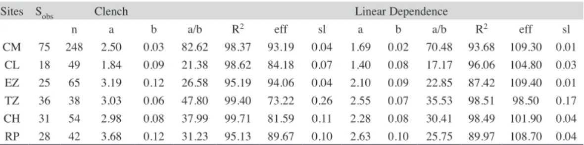
(10) 95.13% (RP) to 99.71% (CH) among streams, and being 98.37% for the CM. The theoretical number of missing species ranged from 2 (EZ) to 13 (TZ) among streams, and 8 for the CM. Curve slopes ranged from 0.04 (EZ) to 0.26 (TZ) among streams, and 0.04 for the CM.. Parametric models: The Clench function fits the data better for each stream and for the CM (Fig. 3, Table 5), with R2 ranging from. Cluster analysis: Colorín (CL) separated first at a major distance (Fig. 4), followed by Ticuiz (TZ). The CL fauna was the poorest,. 90 85 80 75 70 65 60 55 50 45 40 35 30 25 20 15 10 5 0. Clench asymptote. Observed Clench Linear dependence. 1 8 15 22 29 36 43 50 57 64 71 78 85 92 99 106 113 120 127 134 141 148 155 162 169 176 183 190 197 204 211 218 225 232 239. Cumulative number of species. 82.3% and 79.7% sampling efficiencies. These estimators predicted 16 and 19 potential additional species. The best local estimation of richness was made by Chao 1 (EZ, CH, RP) and by Bootstrap (CL, TZ) yielding higher sampling efficiencies.. Sampling effort Fig. 3. Cumulative species curves for Coalcomán Odonata larval assemblage generated by the Clench and Linear Dependence functions. The dashed line is the asymptote estimated by the Clench model.. TABLE 5 Sites, number of species, parameters and predictions of two species accumulation models fitted for each odonate larval assemblage (key to sites in Table 1) Sites. Sobs. CM CL EZ TZ CH RP. 75 18 25 36 31 28. n 248 49 65 38 54 42. Clench a 2.50 1.84 3.19 3.03 2.98 3.68. b 0.03 0.09 0.12 0.06 0.08 0.12. a/b 82.62 21.38 26.58 47.80 37.99 31.23. R2 98.37 98.62 95.19 99.40 99.71 95.13. eff 93.19 84.18 94.06 73.22 81.59 89.67. sl 0.04 0.07 0.04 0.26 0.11 0.10. Linear Dependence a b a/b 1.69 0.02 70.48 1.40 0.08 17.17 2.10 0.09 22.85 2.55 0.07 35.53 2.28 0.08 30.41 2.63 0.10 25.75. R2 93.68 96.06 87.42 98.51 98.49 89.97. eff. 109.30 104.80 109.40 98.50 101.90 108.70. sl. 0.01 0.03 0.01 0.17 0.04 0.04. Sobs=number of observed species, a=the slope to the beginning of sampling, b=a parameter related to the mode of accumulation of new species during sampling, a/b=asymptote, n=total number of samples, R2=coefficient of determination, eff=percentage of efficiency, and sl=slope. The slope was evaluated using the first derivative of Clench’s function [a/ (1+b*n)2] and the first derivative of the Linear Dependence function [a * exp(-b*n)].. 1568. Rev. Biol. Trop. (Int. J. Trop. Biol. ISSN-0034-7744) Vol. 59 (4): 1559-1577, December 2011.

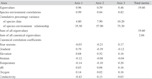
(11) 1.3E-01. 4.5E-01. 100. 75. Distance (Objective Function) 7.6E-01 1.1E+00 Information Remaining (%) 50 25. 1.4E+00 0. EZ RP CH TZ CL Fig. 4. Cluster analysis dendrogram based on Bray-Curtis’ similarity (using the UPGMA Linkage Method) of Odonata larvae collected from the Coalcomán Mountain Range. EZ=Estanzuela, TZ=Ticuiz, RP=Pinolapa, CH=Chichihua and CL=Colorín.. where Hetaerina capitalis dominated (almost 75% of the total abundance), and with many (55.56%) rare species (species with relative abundance less than 1%). TZ was the stream with the largest number of observed species, most (80.56%) of which were rare. Overall turnover rate was less than 25%, except in EZ-RP (48%). Considering the seasonal assemblages, the cluster analysis shows the formation of two groups of contiguous seasons: the first one formed by spring+summer and the second. one for autumn+winter. The first group had the assemblages with the highest number of species and abundance, where the dominant species were the zygopterans Argia pulla, H. capitalis and A. oenea; while in the second group the anisopterans Macrothemis pseudimitans and Erpetogomphus elaps were dominant. Species-environment relationships: The results of CCA were globally significant (trace=2.66, F=4.04, p=0.002, Table 6). The first three axes accounted for most of the. TABLE 6 Results of CCA of log-transformed larval abundance as a function of their environmental variables Axes Eigenvalues Species-environment correlations Cumulative percentage variance of species data of species-environment relationship Sum of all eigenvalues Sum of all canonical eigenvalues Canonical correlation coefficients Year seasons Gradient Elevation Stratum Temperature pH Oxygen Conductivity. Axis 1 0.96 0.99. Axis 2 0.59 0.84. Axis 3 0.46 0.82. 4.80 35.50. 7.90 57.90. 10.20 75.30. -0.03 0.79 0.68 -0.12 -0.14 0.03 0.14 -0.43. -0.21 -0.39 0.52 -0.08 -0.10 0.06 0.02 0.13. 0.17 -0.12 0.16 -0.04 0.20 0.16 0.16 0.03. Rev. Biol. Trop. (Int. J. Trop. Biol. ISSN-0034-7744) Vol. 59 (4): 1559-1577, December 2011. Total inertia 19.60. 19.60 2.66. 1569.

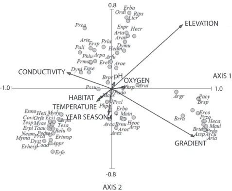
(12) variability (75.3%) for physiochemical variables and species abundance (inertia=19.60). The first canonical axis was statistically significant (eigenvalue=0.945, F=11.90, p=0.002) and explained 35.5% of the variance, while the second and third axes explained 22.4% and 17.4%, respectively. The most important environmental variables explaining larval variation were determined from axis correlations, with gradient and elevation exerting the strongest influence on axes 1 and 2, and axis 1 also influenced by conductivity to yield three putative groups (Fig. 5).. Coenagrionidae predominated (19 and 29 species, respectively) with the genus Argia having the most species (14) (Alonso-Eguía Lis 2004, Gómez-Anaya et al. 2000, Novelo-Gutiérrez & González-Soriano 1991, Novelo-Gutiérrez et al. 2002, Bond et al. 2006). However, some variation in the proportion of Anisoptera to Zygoptera species was observed: while the number of observed Anisoptera species was similar to that for Zygoptera in CH, CL and EZ, in RP and TZ five and nine more Anisoptera species were recorded, respectively. The extreme differences in number of species presented by TZ and CL can be explained because TZ possesses a mixed lotic-lentic environment, is low in altitude, open and sunny, has floating water lilies, Eichhornia crassipes (Mart. Solms), and submerged (Egeria sp.) macrophytes, and is exposed to continuous human impact. Our results could be explained. DISCUSSION As commonly occurs in Mexico, more Anisoptera (62.67%) were observed than Zygoptera (37.33%), and the Libellulidae and. 0.8. ELEVATION. CONDUCTIVITY. pH. -1.0. AXIS 1. OXYGEN. 1.0. HABITAT TEMPERATURE YEAR SEASON GRADIENT. -0.8. AXIS 2 Fig. 5. CCA biplot showing environmental variables (arrows) most strongly correlated with axes CC1 and CC2. Variables include elevation, gradient, conductivity, season, pH, oxygen, temperature, and habitat. Environmental variables providing strong influence on larval assemblage composition have longer arrows than less influential variables.. 1570. Rev. Biol. Trop. (Int. J. Trop. Biol. ISSN-0034-7744) Vol. 59 (4): 1559-1577, December 2011.

(13) by the intermediate disturbance hypothesis (Connell 1978) which states that diversity is low after a disturbance, when only a few species have survived or few colonizing species dominate under the new environmental conditions. Diversity is high when disturbances occur at an intermediate frequency or with intermediate intensity. In this respect, frequent dragging in the TZ channel to extract gravel can be regarded as a disturbance since it alters the habitat. Furthermore, dragging generates medium sized lentic habitats which are mainly occupied by opportunistic libellulids such as Erythrodiplax, Erythemis, Miathyria, Micrathyria, Orthemis, and Perithemis, increasing TZ diversity. CL, on the other hand, is located in a ravine at medium altitude, is small in size and almost fully covered by riparian vegetation, is a stream structured as successive terraces, and has negligible human impact. These results support other studies showing species richness to be positively correlated with stream size and canopy openness (Kinvig & Samways 2000, Clausnitzer 2003, Dijkstra & Lempert 2003, Campbell et al. 2010). The number of species among streams, and their abundance and numeric dominance also exhibited temporal variation. In the dendrogram generated by the CA, abundance and number of species were highest in the spring+summer assemblage, and were dominated by the zygopterans Argia pulla, H. capitalis and A. oenea, while the autumn+winter group had the lowest number of species and abundance was dominated by the anisopterans Macrothemis pseudimitans and Erpetogomphus elaps. The alteration in larval dominance may be related to the presence or absence of predators, with dominance by large anisopterans when predatory fish are absent, and by smaller zygopterans when predatory fish are present (Mikolajewski & Johansson 2004). Large anisopteran larvae are more conspicuous to predators than smaller zygopterans. Our ordering of diversity was based on Renyi’s profiles (Tóthmérész 1995) which have been proposed as an efficient method. for comparisons (Southwood & Henderson 2000), although infrequently used as such on the diversity of aquatic macroinvertebrate assemblages (e.g. Sipkay et al. 2007), and even less so for Odonata assemblages (e.g. Jakab et al. 2002). This lack of use may occur because this method involves more calculations than that for simple diversity indices (Tóthmérész 1995). The idea of ordering diversity was first proposed by Patil & Taillie (1977, 1979) and Solomon (1979). By adding a new dimension to the ecological approach of diversity, it connects with the implications of proposals for diversity conservation that focus on recognizing areas of high diversity. We found this tool useful in comparing the diversity of Odonata larval assemblages within the CM. Using this method, we have shown that diversity at CL was the lowest, and that for CH the highest, with the latter being an ecologically preserved area in the state of Michoacán. Among habitats, Renyi’s profiles showed that the highest diversity occurred along stream margins, compared to riffles or pools, even when stream margins and riffles were almost equal in abundance, 4 044 and 3 905, respectively. Additionally, different dominant species were observed among habitats, with E. elaps mainly recorded from riffles and M. pseudimitans and A. pulla mainly from stream margins. Finally, Renyi’s profiles showed a gradual decrease in seasonal diversity, spring>summer>autumn>winter, without intercrossing of profiles. Beta diversity has been poorly evaluated for Mexican invertebrates (Soberón et al. 2005, Escobar 2005, Favila 2005, Noguez et al. 2005). Species turnover is the least studied and understood component of diversity, even though conservation efforts promote great interest in its evaluation (Gaston & Blackburn 2000). There is an inverse relationship between regional beta diversity and the species distributions in a region (Harrison et al. 1992). If the species from a given region have small areas of distribution, such that sites differ in species composition, then a high beta diversity results. However, if species are widely distributed over most of the region, then sites will be more. Rev. Biol. Trop. (Int. J. Trop. Biol. ISSN-0034-7744) Vol. 59 (4): 1559-1577, December 2011. 1571.

(14) similar to each other in species composition, resulting in low beta diversity (Arita & León-Paniagua 1993, Scott et al. 1999; see also Campbell et al. 2010). In our study, beta diversity was evaluated as the complement of BC, a key element in understanding the relationship between the diversity in the CM (regional or gamma diversity), and diversity of each stream at the local, or alpha level (Cornell & Lawton 1992, Ricklefs & Schluter 1993). Most species showed a restricted distribution in the CM, which suggests a high turnover rate, a conclusion supported by the fact that most of the Bray-Curtis paired similarities were smaller than 25%. Hence, beta diversity is an important component of gamma diversity among these sites (Novelo-Gutiérrez & Gómez-Anaya 2009). Our results also support the betadiverse Mexico hypothesis (Arita & León-Paniagua 1993, Sarukhán et al. 1996), a result of high environmental heterogeneity in the CM. From the point of view of biological conservation, beta diversity is an important component that should be taken into account in the establishment of efficient conservation strategies of particular natural areas and/or species (Scott et al. 1999). Considering that observed gamma diversity for the CM comes from sampling, we estimated the theoretical true gamma by using several non-parametric and parametric richness estimators. We used Clench’s model because it has been used often and it better fits this kind of data. For the non-parametric estimators we used both incidence and abundance data, because there is no strong recommendation for a particular one. According to the sampling efficiency Chao1 performed better for EZ, CH and RP, while Bootstrap performed better for TZ, CL, and over all sampled sites. On the other hand, Clench’s model better fit the data based on the coefficient of determination (R2), and we assessed the completeness of our Odonata larval lists using the slope of the curve at maximum effort for the extrapolation estimators provided by the first derivative of both the Clench and Linear Dependence functions. According to these values, the most complete 1572. lists were those with small slopes, where the increasing rate of species additions tended toward zero. These values agreed well with the fact that sampling effort was highest at EZ (n=65) where the lowest slope was found to be associated with the highest sampling efficiency and just two missing species. On the other hand, the number of species collected at TZ yielded 73.22% efficiency and 12 potentially missing species. These observations agree with the fact that a negative and significant correlation between the number of species collected and slope was observed (r=-0.76, p<0.05), and also between slope and percentage efficiency (r=-0.90, p<0.05). Our CCA results show that larval abundance is primarily associated with elevation and stream slope. This observation is consistent with Hofmann & Mason (2005) and Sato & Riddiford (2008) who observed that current velocity is one of the most important factors related to the distribution and abundance of Odonata. As gradient (slope) increases with elevation, so does current velocity, leading to reduced species richness. Several studies have revealed odonate species richness declines with increasing altitude (Borisov 1987, Samways 1989, Vick 1989, Campbell et al. 2010), and in some places few or no Odonata occur above 2 000m (Laidlaw 1934). However, the size of a regional assemblage over a broad spatial area is a function of slope, latitude and altitude (Corbet 1999), as well as local factors such as stream morphology, aquatic vegetation, riparian coverage and physicochemical variables. The separation of CL first in Fig. 5 could be a result of such local differences. Among the sites surveyed, we found most species at 10m.a.s.l. (TZ), and the fewest at 1 050m.a.s.l. (CL). Campbell et al. (2010) calculated a Pearson correlation coefficient between elevation and species richness for all CM windward sites as r=-0.92 (p>0.05). Even though they revealed a decline with increasing elevation, the marginal insignificance of the correlation was due to the low number of sites surveyed (n=3). Yet, despite the marginal insignificance, average taxonomic distinctness (a measure of. Rev. Biol. Trop. (Int. J. Trop. Biol. ISSN-0034-7744) Vol. 59 (4): 1559-1577, December 2011.

(15) phylogenetic diversity; e.g. Warwick & Clarke 1995, Clarke & Warwick 1998) was significantly and negatively correlated with observed species richness, suggesting the decline in species richness with elevation is real. It is known that altitude-related changes in species composition usually entail a progressive disappearance of the more abundant species at higher altitudes, although some taxa can have their centers of distribution at high and intermediate altitudes (Corbet 1999). In the CM we observed Hetaerina capitalis as the most common species at CL (1 050m, see Table 2), decreasing notably in larval abundance at CH (1 130m), while other species also present at CL such as Progomphus zonatus, Brechmorhoga tepeaca and Macrothemis ultima also decreased or disappeared in CH. Larvae from these four species were not found at lower elevations. We also observed that a higher number of species of Gomphidae (10 out of a total of 13), as well as most of the abundance of this family (more than 90%, but primarily from Erpetogomphus elaps) was recorded at intermediate altitudes, between 408m.a.s.l. and 560m.a.s.l. Notwithstanding, Erpetogomphus elaps was the most abundant and widespread species in the CM, its highest larval abundance occurred at 152m.a.s.l. On the other hand, Libellulidae were better represented with 22 species (from a total of 29) below 560m.a.s.l. Only 12 species from this family were recorded as larvae above 1 000m.a.s.l.; Brechmorhoga tepeaca, Dythemis multipunctata, Macrothemis ultima and Paltothemis cyanosoma were recorded exclusively above 1 000m.a.s.l. In contrast with Hoffmann (1991) who reported a predominance of species of Rhionaeschna (Aeshnidae) at higher elevations in the Peruvian Andes, this family was not well represented in the CM either in number of species or abundance. While most Coenagrionidae species were recorded at CH (11 out of a total of 19); two species, Argia cuprea and A. lacrimans, were exclusively recorded from 1 050m.a.s.l. (CL). Finally, recommendations for the conservation of odonate diversity in the CM are based on the high beta diversity observed and on. stream quality; as shown in the CCA analyses where it was possible to incorporate characteristics of local microhabitats. The conserved vegetation cover and the negligible human impact in CL are, for example, important factors to consider (Buchwald 1992, Remsburg et al. 2008). Alteration of plant cover could change the aquatic microclimate and lead to changes in Odonata diversity (e.g. Samways & Sharratt 2009, Campbell et al. 2010). The CL fauna, although minor in assemblage size, comprises a particular group of infrequent species: Argia cuprea, A. lacrimans, Aeshna williamsoniana and Paltothemis cyanosoma, all of which occurred uniquely in this locality. Other species such as Hetaerina capitalis, Erpetogomphus cophias, Progomphus zonatus, Brechmorhoga tepeaca and Macrothemis ultima have their maximum and almost exclusive records at this site. It is feasible that their association with stream slope may be based on associations with conserved canopy, small size, shallow runs, small to moderate sized pools and sand banks with rough grains. This opens some questions: What is the importance of the ravines like CL as shelters for these infrequent species in a broader scale (e.g. in all the Michoacán Mountain Ranges?) Are the odonate assemblages different in each ravine increasing the beta diversity? Our results support the suggestion for locally based conservation efforts along the windward transect (e.g. Campbell et al. 2010), and support proposals describing the CM as a biologically rich area for conservation. ACKNOWLEDGMENTS Financial support was provided to RNG by Comisión Nacional de Ciencia y Tecnología (CONACyT) grant 43091-Q. RESUMEN Evaluar los componentes de la diversidad de paisaje es una tarea esencial para implementar estrategias eficientes de conservación. En este estudio se describe la variación geográfica, temporal y por hábitats de la diversidad de larvas de odonatos en un gradiente altitudinal en la sierra de. Rev. Biol. Trop. (Int. J. Trop. Biol. ISSN-0034-7744) Vol. 59 (4): 1559-1577, December 2011. 1573.

(16) Coalcomán, Michoacán, México, y se explora su relación con variables fisicoquímicas locales. Presentamos diferentes índices de diversidad y gráficos de perfiles de diversidad de Renyi, así como la riqueza teórica por métodos paramétricos y no paramétricos, el recambio de especies en la sierra y, mediante análisis canónico de correspondencias (ACC) la relación de las especies con las variables fisicoquímicas. Recolectamos un total 12 245 larvas de 75 especies, 28 géneros y 8 familias. En todos los hábitats un alto número de especies presentó una abundancia inferior al 1%. El número de especies en los arroyos varió entre 18 y 36, existe además un alto recambio en la sierra. La diversidad beta es un componente importante de la diversidad del paisaje; se apreció una alternancia en la dominancia estacional entre anisópteros y zygópteros y nuestros datos concuerdan con la hipótesis del Mexico betadiverso y también apoya propuestas previas de conservación de la sierra. Palabras clave: Odonata, larvas, diversidad, ACC, Sierra de Coalcomán, Michoacán, México.. REFERENCES Alonso-Eguía Lis, P.E. 2004. Ecología de las asociaciones de Odonata en la zona de influencia de las microcuencas afectadas por la presa Zimapán, Querétaro e Hidalgo. Tesis Doctoral, Universidad Autónoma de Querétaro, México. Antaramián, H.E. 2005. Descripción física y biótica. Clima, p. 25-28. In L.E. Villaseñor-G (ed.). La Biodiversidad en Michoacán. Estudio de Estado. CONABIO-SUMA-MSNH, México. Arita, H.T. & L. León-Paniagua. 1993. Diversidad de mamíferos terrestres. Ciencias (número especial) 7: 13-22. Arriaga, L., V. Aguilar, J. Alcocer, R. Jiménez, E. Muñoz & E. Vázquez. 1998. Regiones hidrológicas prioritarias. Escala de trabajo 1:4 000,000. Comisión Nacional para el Conocimiento y Uso de la Biodiversidad, México. Arriaga, L., J.M. Espinoza, C. Aguilar, E. Martínez, L. Gómez & E. Loa. 2000. Regiones terrestres prioritarias de México. Escala de trabajo 1:1 000,000. Comisión Nacional para el Conocimiento y Uso de la Biodiversidad, México. Bond, J.G., R. Novelo-Gutiérrez, A. Ulloa, J.C. Rojas, H. Quiroz-Martínez & T. Williams. 2006. Diversity, abundance, and disturbance response of Odonata associated with breeding sites of Anopheles pseudopunctipennis (Diptera: Culicidae) in Southern Mexico. Environ. Entomol. 35: 1561-1568.. 1574. Borisov, S.M. 1987. Ecology of two closely related dragonfly species in Tajikistan. Ekologiya 1: 85-87. Bried, J.T., B.D. Herman & G.N. Ervin. 2007. Umbrella potential of plants and dragonflies for wetland conservation: a quantitative case study using the umbrella index. J. Appl. Ecol. 44: 833-842. Buchwald, R. 1992. Vegetation and dragonfly fauna characteristics and examples of biocenological field studies. Vegetatio 101: 99-107. Bulánková, E. 1997. Dragonflies (Odonata) as bioindicators of environmental quality. Biológia (Bratislava) 52: 177-180. Campbell, W.B. & R. Novelo-Gutiérrez. 2007. Reduction in odonate phylogenetic diversity associated with dam impoundment is revealed using taxonomic distinctness. Fund. Appl. Limnol. 168: 83-92. Campbell, W.B., R. Novelo-Gutiérrez & J.A. Gómez-Anaya. 2010. Distributions of odonate richness and diversity with elevation depend on windward and leeward aspects: implications for research and conservation planning. Insect. Conserv. Diver. 3: 302-312. Carchini, G. & E. Rota. 1985. Chemico-physical data on the habitats of rheophile Odonata from Central Italy. Odonatologica 14: 239-245. Carle, F.L. 1979. Environmental monitoring potential of the Odonata, with a list of rare and endangered Anisoptera of Virginia, United States. Odonatologica 8: 319-323. Castella, E. 1987. Larval Odonata distribution as a describer of fluvial ecosystems: the Rhône and Ain Rivers, France. Adv. Odonatol. 3: 23-40. Chovanec, A. & J.A. Waringer. 2001. Ecological integrity of river floodplain systems - assessment by dragonfly surveys (Insecta: Odonata). Regul. Rivers 17: 493-507. Clark, T.E. & M.J. Samways. 1996. Dragonflies (Odonata) as indicators of biotope quality in the Kruger National Park, South Africa. J. Appl. Ecol. 33: 1001-1012. Clarke, K.R. & R.M. Warwick. 1998. A taxonomic distinctness index and its statistical properties. J. Appl. Ecol. 35: 523-531. Clausnitzer, V. 2003. Dragonfly communities in coastal habitats of Kenya: indication of biotope quality and the need of conservation measures. Biodivers. Conserv. 12: 333-356.. Rev. Biol. Trop. (Int. J. Trop. Biol. ISSN-0034-7744) Vol. 59 (4): 1559-1577, December 2011.

(17) Clench, H. 1979. How to make regional lists of butterflies: some thoughts. J. Lepid. Soc. 33: 216-231. Colwell, R.K. 2006. EstimateS: statistical estimation of species richness and shared species from samples. Version 8.0. Department of Ecology and Evolutionary Biology, University of Connecticut, USA. (User’s guide and application published at: http:// purl.oclc.org/estimates). Connell, J.H. 1978. Diversity in tropical rain forests and coral reefs. Science 199: 1304-1310. Corbet, P.S. 1999. Dragonflies. Behaviour and ecology of Odonata. Cornell University, Ithaca, New York, USA. Cornell, H.V. & J.H. Lawton. 1992. Species interactions, local and regional processes, and limits to the richness of ecological communities: a theoretical perspective. J. Anim. Ecol. 61: 1-12. D’Amico, F., S. Darblade, S. Avignon, S. Blanc-Manel & S.J. Ormerod. 2004. Odonates as indicators of shallow lake restoration by liming: comparing adult and larval responses. Restor. Ecol. 12: 439-446. Dijkstra, K-D.B. & J. Lempert. 2003. Odonate assemblages of running waters in the Upper Guinean forest. Arch. Hydrobiol. 157: 397-412. Escobar, F. 2005. Diversidad, distribución y uso de hábitat de los escarabajos del estiércol (Coleoptera: Scarabaeideae: Scarabaeinae) en montañas de la Región Neotropical. Tesis de Doctorado, Instituto de Ecología, A.C, Xalapa, México. Favila, M.E. 2005. Diversidad alfa y beta de los escarabajos del estiércol (Scarabaeinae) en Los Tuxtlas, México, p. 209-219. In G. Halffter, J. Soberón, P. Koleff & A. Melic. Sobre diversidad biológica: el significado de las diversidades alfa, beta y gamma. Monografías Tercer Milenio, Sociedad Entomológica Aragonesa, Zaragoza, España. Ferreras-Romero, M. 1988. New data on the ecological tolerance of some rheophilous Odonata in Mediterranean Europe (Sierra Morena, Southern Spain). Odonatologica 17: 121-126. Foote, A.L. & C.L.R. Hornung. 2005. Odonates as biological indicators of grazing effects of Canadian prairie wetlands. Ecol. Entomol. 30: 273-283. Fraser, D.M.S., R.M. May, R. Pellew, T.H. Johnson & K.R. Walter. 1993. How much do we know about the current extinction rate? Trends Ecol. Evol. 8: 75-378.. Gaston, K.J. & T.M. Blackburn. 2000. Pattern and process in Macroecology. Blackwell Science, Oxford, United Kingdom. Gentry, J.B., C.T. Garten, F.G. Howell & M.H. Smith. 1975. Thermal ecology of dragonflies in habitats receiving reactor effluent, p. 563-574. In Environmental effect of cooling systems at nuclear power plants. International Atomic Energy Agency, Vienna, Austria. Gómez-Anaya, J.A., R. Novelo-Gutiérrez & R. Arce-Pérez. 2000. Odonata de la zona de influencia de la Central Hidroeléctrica “Ing. Fernando Hiriart Balderrama” (P.H. Zimapán), Hidalgo, México. Folia Entomol. Mexic. 108: 1-34. Gupta, A. 1995. Metal accumulation and loss by Crocothemis servilia (Drury) in a small lake in Shillong northeastern India (Anisoptera: Libellulidae). Odonatologica 24: 283-289. Harrison, S., S. Ross & J.H. Lawton. 1992. Beta diversity on geographic gradients in Britain. J. Anim. Ecol. 67: 151-158. Hawking, J.H. & T.R. New. 2002. Interpreting dragonfly diversity to aid in conservation assessment: lessons from the Odonata assemblage at Middle Creek, north-eastern Victoria, Australia. J. Insect. Conservat. 6: 171-178. Hoffmann, J. 1991. The distribution of the aeshnids (Anisoptera) in the Peruvian Andes. In 11th International Symposium of Odonatology, Trevi, Italia. Hofmann, T.A. & C.F. Mason. 2005. Habitat characteristics and the distribution of Odonata in a lowland river catchment in eastern England. Hydrobiologia 539: 137-147. Hornung, J.P. & C.L. Rice. 2003. Odonata and wetland quality in southern Alberta, Canada: a preliminary study. Odonatologica 32: 119-129. Hortal, J. & J.M. Lobo. 2005. An ED-based protocol for optimal sampling of biodiversity. Biodivers. Conserv. 14: 2913-2947. Hurtado-González, S., M.A. Rico & P.J. Gutiérrez-Yurrita. 2001. Efecto del Malatión (insecticida organofosforado) sobre los insectos acuáticos de los afluentes de la Presa Zimapán, Querétaro-Hidalgo. XXX Congreso Nacional de Ciencias Fisiológicas, Monterrey, Nuevo León, México. Jakab, T., Z. Müller, G.Y. Dévai & B. Tóthmérész. 2002. Dragonfly assemblages of a shallow lake type. Rev. Biol. Trop. (Int. J. Trop. Biol. ISSN-0034-7744) Vol. 59 (4): 1559-1577, December 2011. 1575.

(18) reservoir (Tisza-Tó, Hungary) and its surroundings. Acta Zool. Hung. 48: 161-171. Jiménez-Valverde, A. & J. Hortal. 2003. Las curvas de acumulación de especies y la necesidad de evaluar la calidad de los inventarios biológicos. Rev. Ibér. Arachnol. 8: 151-161.. Novelo-Gutiérrez, R., J.A. Gómez-Anaya & R. Arce-Pérez. 2002. Community structure of Odonata larvae in two streams in Zimapán, Hidalgo, Mexico. Odonatologica 31: 273-286. Palmer, M.W. 1990. The estimation of species richness by extrapolation. Ecology 71: 1195-1198.. Kinvig, R.G. & M.J. Samways. 2000. Conserving dragonflies (Odonata) along streams running through commercial forestry. Odonatologica 29: 195-208.. Patil, G.P. & C. Taillie. 1977. Diversity as a concept and its implications for random communities. Bull. Int. Stat. Inst. 47: 497-515.. Laidlaw, F.F. 1934. Notes on some Oriental dragonflies (Odonata), with description of a new species. Stylops 3: 99-103.. Patil, G.P. & C. Taillie. 1979. An overview of diversity, p. 3-27. In J.F. Grassle, G.P. Patil, W. Smith & C. Taillie (eds.). Ecological diversity in theory and practice. International Cooperative, Fairland, Maryland, USA.. McCune, B. & J.B. Grace. 2002. Analysis of ecological communities. MjM Software, Gleneden Beach, Oregon, USA. McGeoch, M.A. 1998. The selection, testing and application of terrestrial insects as bioindicators. Biol. Rev. 73: 181-201. Mittermeier, R.A., N. Myers & J.B. Thomsen. 1998. Biodiversity hotspots and major tropical wilderness areas: approaches to setting conservation priorities. Conservat. Biol. 12: 516-520. Mikolajewski, D.J. & F. Johansson. 2004. Morphological and behavioral defenses in dragonfly larvae: trait compensation and cospecialization. Behav. Ecol. 4: 614-620. Moore, N.W. 1997. Status survey and conservation action plan. Dragonflies. IUCN/SSC Odonata Specialist Group, IUCN, Gland and Cambridge, United Kingdom. Moreno, C.E. 2001. Métodos para medir la biodiversidad. M&T-Manuales y Tesis SEA, Zaragoza, España. Noguez, A.M., H.T. Arita, A.E. Escalante, L.J. Forney, F. García-Oliva & V. Souza. 2005. Microbial macroecology: highly structured prokaryotic soil assemblages in a tropical deciduous forest. Global Ecol. Biogeogr. 14: 241-248. Novelo-Gutiérrez, R. & E. González-Soriano. 1991. Odonata de la Reserva de la Biosfera “La Michilía”, Durango, México. Parte II. Larvas. Folia Entomol. Mex. 81: 107-164. Novelo-Gutiérrez, R. & J.A. Gómez-Anaya. 2009. A comparative study of Odonata (Insecta) assemblages along an altitudinal gradient in the Sierra de Coalcomán Mountains, Michoacán, Mexico. Biodivers. Conserv. 18: 679-698.. 1576. Remsburg, A.J., A.C. Olson & M.J. Samways. 2008. Shade alone reduces adult dragonfly (Odonata: Libellulidae) abundance. J. Insect Behav. 21: 460-468. Resh, V.H., M.J Myers & M.J. Hannaford. 1996. Macroinvertebrates as biotic indicators of environmental quality, p. 647-655. In F.R. Hauer & G.A. Lamberti. Methods in stream ecology. Academic, London, United Kingdom. Ricklefs, R.E. & D. Schluter. 1993. Species diversity in ecological communities, historical and geographical perspectives. University of Chicago, Chicago, USA. Rodríguez, J.I. 2003. Asimilación de plomo por la comunidad del macrobentos del área de influencia hidrológica de la presa Zimapán y su importancia en la transmisión de este xenobiótico a la tilapia Oreochromis mossambicus. Tesis de Licenciatura, Universidad Autónoma de Querétaro, Querétaro, México. Sahlén, G. & K. Ekestubbe. 2001. Identification of dragonflies (Odonata) as indicators of general species richness in boreal forest lakes. Biodivers. Conserv. 10: 673-690. Samways, M.J. & N.J. Sharratt. 2009. Recovery of endemic dragonflies after removal of invasive alien trees. Conservat. Biol. 24: 267-277. Samways, M.J. 1989. Taxon turnover in odonates across a 3000 m altitudinal gradient in southern Africa. Odonatologica 18: 263-274. Samways, M.J. 1993. Dragonflies (Odonata) in taxic overlays and biodiversity conservation, p. 111-123. In K.L. Gaston, T.R. New & M.J. Samways (eds.). Perspectives in insect conservation. Intercept, Andover, United Kingdom. Sarukhán, J., J. Soberón & J. Larson-Guerra. 1996. Biological conservation in a high beta diversity country,. Rev. Biol. Trop. (Int. J. Trop. Biol. ISSN-0034-7744) Vol. 59 (4): 1559-1577, December 2011.

(19) p. 246-263. In E. di Castri & T. Younes (eds.). Biodiversity, science and development: toward a new partnership. CAB International-IUBS, Paris, France.. StatSoft. 2006. STATISTICA (data analysis software system and computer program manual) Version 7.1. StatSoft Inc., Tulsa, Oklahoma, USA.. Sato, M. & N. Riddiford. 2008. A preliminary study of the Odonata of S’Albufera Natural Park, Mallorca: status, conservation priorities and bio-indicator potential. J. Insect Conservat. 12: 539-548.. Takamura, K., S. Hatakeyama & H. Shiraishi. 1991. Odonatae larvae as an indicator of pesticide contamination. Appl. Entomol. Zool. 26: 321-326.. Scott, J.M., E.A. Norse, H.T. Arita, A. Dobson, J.A. Estes, M. Foste, B. Gilbert, D. Jensen, R.L. Knight, D. Mattson & M.E. Soulé. 1999. The issue of scale in selecting and designing biological reserves, p. 19-37. In M.E. Soulé & J. Terborgh (eds.). Continental Conservation, Scientific Foundations of Regional Reserve Networks. Island, Washington, D.C., USA. Sipkay, C.S., L. Hufnagel, A. Révész & G. Petrányi. 2007. Seasonal dynamics of an aquatic macroinvertebrate assembly (Hydrobiological case study of Lake Balaton, No. 2). Appl. Ecol. Environ. Res. 5: 63-78. Smith, J., M.J. Samways & S. Taylor. 2007. Assessing riparian quality using two complementary sets of bioindicators. Biodivers. Conserv. 16: 2695-2713. Soberón, J. & J. Llorente. 1993. The use of the species accumulation functions for the prediction of species richness. Conservat. Biol. 7: 480-488. Soberón, J., J. Llorente & A.M. Luis. 2005. Estimación del componente beta del número de especies de Papilionidae y Pieridae (Insecta: Lepidoptera) de México por métodos indirectos, p. 231-237. In G. Halffter, J. Soberón, P. Koleff & A. Meliá (eds.). Sobre diversidad biológica: el significado de las diversidades alfa, beta y gamma. Monografías Tercer Milenio, Bol. Soc. Ent. Aragones, Zaragoza, España. Solomon, D.L. 1979. A comparative approach to species diversity, p. 29-35. In J.F. Grassle, G.P. Patil, W. Smith & C. Taillie (eds.). Ecological diversity in theory and practice. International Cooperative Publishing House, Fairland, Maryland, USA. Southwood, T.R.E. & P.A. Henderson. 2000. Ecological methods. Blackwell, Oxford, United Kingdom.. ter Braak, C.J.F. 1986. Canonical correspondence analysis: a new eigenvector technique for multivariate direct gradient analysis. Ecology 67: 1167-1179. ter Braak, C.J.F. & I.C. Prentice. 1988. A theory of gradient analysis. Adv. Ecol. Res. 18: 271-313. ter Braak, C.J.F. & P. Smilauer. 2002. Canoco for Windows Version 4.5. Biometrics - Plant Research International, Wageningen, The Netherlands. Thorp, J.H. & M.R. Diggins. 1982. Factors affecting depth distribution of dragonflies and other benthic insects in a thermally destabilized reservoir. Hydrobiologia 87: 33-44. Tóthmérész, B. 1995. Comparison of different methods for diversity ordering. J. Veg. Sci. 6: 283-290. Tóthmérész, B. 1998. On the characterization of scaledependent diversity. Abstracta Botanica 22: 149-156. Trevino, J. 1997. Dragonflies [sic] naiads as an indicator of water quality. Center for Watershed Prot., Silver Spring, MD, U.S. Environ. Prot. Agency. Tech. Note 99, Watershed Protection Techniques 2: 533-535. Vick, G.S. 1989. List of the dragonflies recorded from Nepal, with a summary of their altitudinal distribution (Odonata). Opusc. Zool. Flumin. 43: 1-21. von Bertalanffy, L. 1938. A quantitative theory of organic growth. Hum. Biol. 10: 181-213. Warwick, R.M. & K.C. Clarke. 1995. New “biodiversity” measures reveal a decrease in taxonomic distinctness with increasing stress. Mar. Ecol. Prog. Ser. 129: 301-305. Watson, J.A.L., A.H. Arthington & D.L. Conrick. 1982. Effect of sewage effluent on dragonflies (Odonata) of Bulimba Creek, Brisbane. Aust. J. Mar. Freshwat. Res. 33: 517-528.. Rev. Biol. Trop. (Int. J. Trop. Biol. ISSN-0034-7744) Vol. 59 (4): 1559-1577, December 2011. 1577.

(20)

(21)