Unbounded growth in the Neoclassical growth model with
non-constant discounting
Francisco Cabo1, Guiomar Mart´ın-Herr´an2,∗, Mar´ıa Pilar Mart´ınez-Garc´ıa3,∗
Abstract
For a Neoclassical growth model, the literature highlights that exponential discounting is observationally equivalent to quasi-hyperbolic discounting, if the instantaneous discount rate decreases asymptotically towards a positive value. Conversely, in this paper a zero long-run value allows a solution without stagnation. We prove that a less than exponential but unbounded growth can be attained, even without technological progress. The growth rate of consumption decreases asymptotically towards zero, although so slowly that consumption grows unboundedly. The asymptotic convergence towards a non-hyperbolic steady-state which saving rate matches the intertemporal elasticity of substitution and the speed of convergence towards this equilibrium are analyzed.
JEL Classification: O40, C61, C62, D90.
Keywords Non-constant discounting; less than exponential unbounded growth; non-hy-perbolic equilibrium; center manifold.
1. Introduction
The way individuals discount the future plays an important role in intertemporal decision making and, in consequence, it may have an impact on economic growth. This paper aims to prove that non-exponential discounting facilitates the appearance of patterns of growth distinct from the standards in a Neoclassical growth model without technological change.
∗
Corresponding author: Dpto. Econom´ıa Aplicada (Matem´aticas), Universidad de Valladolid, Avda. Valle de Esgueva, 6, 47011, Valladolid, Spain. Tel.: +34 983 423330 Fax: +34 983 423299; e-mail: [email protected]
1
IMUVA, Universidad de Valladolid, Spain. Dpto. Econom´ıa Aplicada (Matem´a ticas), Universi-dad de Valladolid, Avda. Valle de Esgueva, 6, 47011, Valladolid, Spain. Tel.: +34 983 186662 e-mail: [email protected]
2
IMUVA, Universidad de Valladolid, Spain 3
More specifically, this paper shows that the hypothesis of consumers discounting the future at non-constant rates might help to avoid stagnation even if technological progress is nil. In particular, this hypothesis makes a new pattern of growth feasible somewhere in between stagnation (the standard outcome in Neoclassical growth models) and exponential growth (obtained in endogenous growth models).
This less than exponential pattern of growth in a Neoclassical growth model has been analyzed in the literature through the concept of quasi-arithmetic growth. This type of growth is characterized by a rate of decline of the growth rate proportional to itself. Under this regularity condition economic growth is unbounded although the growth rate of the economy decreases asymptotically towards zero. Quasi-arithmetic growth was first intro-duced by Mitra (1983) and later developed by Asheim et al. (2007), Pezzey (2004) and Groth et al. (2010). The existence of this type of growth relies on the assumption of a quasi-arithmetic technical progress in the long-run.
In our paper the center of gravity moves from production or technology to time prefer-ences. We discard any source of long-run growth such as technology or population growth and focus on human impatience. We prove that, if consumers discount the future at a non-constant rate, less than exponential growth in a Neoclassical growth model is feasible even if technical progress is nil. Moving away from the standard assumption of a constant rate of time preference we adopt the empirically supported hypothesis of non-constant discounting with decreasing impatience. Specifically, we assume an instantaneous time discount rate which decreases towards zero with the time-distance from the present.
There exists a wide consensus on the appropriateness of time-varying discount rates.4 According to Laibson (1997), individuals are highly impatient about consumption in the near future, but much more patient when confronted with choices in the distant future. However, time-varying discount rates have not been widely used in economics because they imply an important drawback: the time-inconsistency problem. With non-constant dis-counting, preferences change with time and committed choices typically differ from those chosen sequentially (this had already been pointed out by Ramsey 1928 and later by Strotz 1956, Pollak 1968 and Goldman 1980).5 One way to solve this problem is to consider a
so-4
A very interesting discussion on time discounting can be found in Frederick et al. (2002). The opinion that a non-constant discounting better fits reality is not unanimous in the literature, see, for example, Andersen et al. (2014) for a recent criticism.
5
phisticated agent that, being aware that he cannot precommit his future behavior, adopts a strategy of optimal planning against its future self, a game among a succession of future planners. Using this approach, Karp (2007) proposed a method for analyzing the solutions in a non-constant discounting infinite time horizon setting, and Mar´ın-Solano and Navas (2009) extended the results to a non-constant discounting finite horizon problem.
In his seminal paper, Barro (1999) introduces a varying rate of time preference in a Neoclassical growth model with sophisticated agents to avoid time-inconsistency.6 The in-stantaneous time discount rate decreases with the time-distance from the present, and it is assumed that it converges towards a positive constant. The consequence of this assump-tion of quasi-hyperbolic discounting is that, the model is observaassump-tionally equivalent7 to the standard Neoclassical growth model with a positive constant rate of time preference. In consequence, stagnation is the forced outcome in the long-term if exogenous technological improvements are absent. In this paper, we also consider a sophisticated agent but, unlike Barro (1999), we assume that the instantaneous time discount rate asymptotically declines towards zero. Our assumption means that a present individual does not discount a delay in the very distant future. This hypothesis is already present in the hyperbolic discount functions proposed in the classical psychological literature (Ainslie, 1992). Moreover this property is characteristic of many discount functions proposed in the economic literature on non-constant discounting, like, for example, hyperbolic discounting, proportional dis-counting, power discounting and constant sensitivity (see, Abdellaoui et al. 2010). In a continuous setting, a time-varying discount rate asymptotically converging to zero also ap-pears in the logarithmic discounting proposed by Heal (2007) (and considered by Heal 1998 and Li and Lofgren 2000 to analyze sustainable resource management), and in the regular discounting used by Pezzey (2004) and Farzin and Wendner (2014). Moreover, we assume that the discount function never vanishes, meaning that individuals are not shortsighted in the sense that they do not disregard long-term consequences. Under these assumptions, our model predicts similar results to those of the Neoclassical growth model with a zero time-discount rate.
and Silverman (2009), Fang and Wang (2015).
6For endogenous growth models, the effects of a time-varying discount rate on long-run growth is analyzed in Strulik (2014) and Cabo et al. (2015).
7
Our first aim is, therefore, to analyze the benchmark Neoclassical growth model without technological change and with a zero time-discount rate. The Neoclassical hypothesis of de-creasing returns to capital implies an ever dede-creasing rate of return on capital and, therefore, a continuously decreasing growth rate of consumption. However, if population is constant and the capital depreciation rate is null (or a net-of-capital-depreciation production func-tion is assumed), a regular or quasi-arithmetic growth is obtained.8 Under this regularity condition it can be analytically proved that the growth rate of the economy decays towards zero, but this decay is so slow that consumption grows asymptotically unbounded.
The general model we propose in this paper, with a non-constant discount rate converg-ing asymptotically towards zero, avoids stagnation under conditions equivalent to those in the benchmark model. The economy grows at a decreasing rate converging towards zero, but again consumption grows asymptotically unbounded. We find that the neoclassical economy, when consumers show non-constant time discounting, can be described by a four autonomous differential-equation system. This system presents non-hyperbolic asymptotic equilibria for which the standard techniques to study non-linear dynamical systems are not applicable. The trajectories converging towards the equilibria lie on a center manifold. By analyzing the dynamics within this manifold we manage to prove that, even though the pattern of growth displayed by our general model is not quasi-arithmetic (the regularity condition is not satisfied), it shares the two main properties of this type of growth. First, from a given time on, the growth rate remains positive while decreasing asymptotically towards zero (less than exponential growth); and second, the decay in the growth rate is so slow as to ensure an unlimited amount of consumption as time goes to infinity (unbounded growth). Thus, we call this new pattern of growth less than exponential unbounded growth (LEUG).
The benchmark Neoclassical growth model without discounting is studied in Section 2. In Section 3 we analyze the general model with non-constant discounting. Both problems are solved taking into account the catching-up optimality criterium. Finally, Section 4 concludes. All proofs are given in the Appendix.
2. Neoclassical growth model with a zero time-discount rate
As commented on the introduction, in order to have a better insight of the pattern of growth under non-constant discounting with an instantaneous time discount rate converging towards zero, we start by analyzing the Neoclassical growth model without technological change in the extreme case of a zero time-discount rate.
As is well known (see, for example, Barro and Sala-i-Martin 2004 or Acemoglu 2009), the Neoclassical growth model with a Cobb-Douglas production function and a isoelastic utility function is driven by two equations:9
˙
k=f(k)−c−(n+δ)k=Akα−c−(n+δ)k, k(0) =k0, (1)
γc≡
˙
c c =
1
σ
f0(k)−(δ+ρ)= 1
σ
αAkα−1−(δ+ρ), (2)
with k(t) capital per capita, c(t) consumption per capita, and constant A > 0 the total factor productivity. Constantsn≥0 the growth rate of population,δ ≥0 the depreciation rate of capital, α ∈ (0,1) the output elasticity of capital, k0 ≥ 0 the initial capital per capita, σ > 0 the inverse of the intertemporal elasticity of substitution, and ρ ≥ 0 the instantaneous time-discount rate.
In this section we center our analysis on the extreme case with a zero time-discount rate, ρ = 0. Since the objective function could be unbounded, we use the catching-up optimality criterium (see, for example, Sydster and Seierstad 1987). First-order conditions for optimality are given by equations (1) and (2), together with the transversality condition:
lim
t→∞infµ(t)[˜k(t)−k(t)]≥0,
for all admissible ˜k(t), whereµ(t) =c(t)−σ is the shadow price of the capital per capita for the representative consumer.
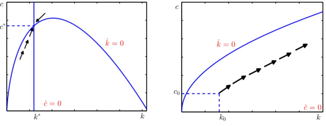
With a zero discount rate, the well-known phase diagram of the Neoclassical growth model (left graph in Figure 1) is still valid. The ˙k = 0 locus is described by the curve
c=Akα−(n+δ)k, and the ˙c= 0 locus by the curves k=k∗ ≡(Aα/δ)1/(1−α) and c= 0. This diagram depicts a unique steady-state saddle point with positive consumption. If the capital per capita is initially low, the transitional dynamics is characterized by growing
9Time argument is omitted henceforth when no confusion can arise. γ
c denotes the growth rate of
consumption and capital per capita, converging towards their steady-state values. In con-sequence, in the absence of technological progress, the assumption of a zero discount rate in the standard model with diminishing returns in capital per capita does not modify the standard result: the growth in capital per worker must necessarily come to a halt; it cannot grow unboundedly.
Nevertheless, stagnation is no longer the obliged outcome under the assumptions of constant population, n= 0, and a net-of-capital production function, δ = 0. In the phase diagram in Figure 1 (right), the ˙k = 0 locus is now concave, although ever-increasing, functionc=Akα. Meanwhile, the ˙c= 0 locus is exclusively defined by the horizontal-axis
c= 0, which cannot be reached ifc0 >0. Thus, given the initial capital stock, if consumption does not exhaust all output, capital starts growing and it might continue growing as long as the economy remains below the ˙k = 0 locus. Correspondingly, consumption would grow at a strictly positive rate, proportional to the marginal productivity of capital per capita. Since technology exhibits diminishing returns to scale, increments in capital would induce a continuous reduction in its marginal productivity and hence on the growth rate of consumption.
c
k c∗
k∗
˙
k= 0
˙
c= 0
c
k ˙
k= 0
c0
k0
˙
c= 0
Figure 1: Phase diagramsk−c;ρ= 0, n, δ >0 (left);ρ=n=δ= 0 (right)
To analyze the feasibility of this type of solution, we first write the system dynamics (1)-(2) in the particular caseρ=δ =n= 0:
˙
k=f(k)−c=Akα−c, k(0) =k0, (3)
γc=
f0(k)
σ = αA
σ k
α−1
Definingsas the share of savings, s∈[0,1], the consumption can be written as
c= (1−s)f(k) = (1−s)Akα, (5)
and defining
r=f0(k) =αAkα−1 (6) as the rate of return of capital, then system (3)-(4) can be rewritten as:
˙
r = −1−α
α sr
2, r(0) =r0 =αAkα−1
0 , (7)
˙
s = −(1−s)
1
σ −s
r. (8)
From equation (8) the ˙s= 0 locus is defined by the vertical-axisr = 0, and the horizontal straight liness= 1 ands= 1/σ. The ˙r = 0 locus is defined by the horizontal (s= 0) and the vertical (r= 0) axes.
Under the assumption σ >1 we study the phase diagram in variablesr−sin Figure 2 which is equivalent to the phase diagram in variables k−c in system (3)-(4). There exist infinitely many possible equilibria located in the unit interval between the origin and point E = (0,1). By computing the integral curves it can be shown that point E is a stable equilibrium for any initial situation with s0 ∈ (1/σ,1) and r0 > 0. The equilibria (0, s∗) withs∗∈[0,1), s∗ = 16 /σ are unstable. The equilibriumEσ = (0,1/σ) is saddle-path stable and it will only be reached if the saving rate lies initially at s0 = 1/σ. Alternatively the same analysis for σ <1 shows that there is no stable equilibrium satisfying s∈ [0,1]. In consequence, here and henceforth, we make the frequent assumption in the literature, of
σ >1.
r s
•
•
˙ r= 0 ˙
r= 0
˙ s= 0
˙ s= 0 ˙
s= 0
1 σ 1
0 0
E I
Eσ I
If the saving rate initially matches the intertemporal elasticity of substitution, s(0) =
s0= 1/σ,it remains constant and equation (3) can be written as the fundamental dynamic equation in the Solow-Swan model, ˙k = Ak1−(1−α)/σ. This is an autonomous Bernoulli
equation whose solution reads
k(t) =k0
1 +γ01−α α t
1−1α
, withγ0= αA
σ k
α−1
0 . (9)
Note that γ0 is the growth rate of consumption at t= 0, then from equations (4) and (5) immediately follows:
γc(t) =
γ0
1 +γ01−α α t
, (10)
c(t) =c0
1 +γ01−α α t
1−αα
, withc0 = σ−1
σ Ak
α
0. (11)
Note thatc0 is the consumption att= 0 when s0 = 1/σ.
The growth rate of consumption in equation (10) fulfils the regularity condition for a quasi-arithmetic growth path ˙γc=−(1−α)/αγc2(for example, in Groth et al. (2010)). This
pattern of growth satisfies that the decay in the growth rate is so slow that both capital and consumption grow unboundedly as time goes to infinity. Trajectories for consumption and capital would collapse in the exponential case as α tends to 1.
From (9) and (11) it is easy to verify that the condition limt→∞µ(t)k(t) = 0, sufficient
to guarantee the transversality condition, is satisfied under condition 1/σ < α, which states that the output elasticity of capital surpasses the intertemporal elasticity of substitution. If this condition is not fulfilled, the output grows too slowly with the capital stock, or the marginal utility decays too slowly with consumption. In either case the capital stock as time goes to infinity would be positively valued. This could mean that the economy should have accumulated more capital.
These results are summarized in the following proposition.
Proposition 1. If s0 = 1/σ, then s(t) remains constant, lim
t→∞r(t) = limt→∞γc(t) = 0 and k
and c grow following a regular pattern with lim
t→∞k(t) = limt→∞c(t) =∞.
Proposition 2. If s0 >1/σ, then lim
t→∞s(t) = 1, and tlim→∞r(t) = limt→∞γc(t) = 0. Moreover, r(t) and γc(t) converge towards zero as function t−1, hence lim
t→∞k(t) = limt→∞c(t) = ∞.
However these trajectories are suboptimal.
From this proposition follows that the solution given in (11) with s(t) = 1/σ for all
t ≥ 0 is the unique solution to the Neoclassical growth without technological change and model with a zero time-discount rate; and this solution displays a regular growth path. The next section analyzes the more general model in which, while maintaining the assumptions of constant population and no capital depreciation, we give entrance to impatience in the consumers’ preferences. We consider individuals whose discount rate decreases as the time distance from the present widens. The question would be whether a similar pattern of unlimited growth could emerge. In particular, we study the conditions under which the growth rate of consumption, although tending towards zero, allows consumption to grow unboundedly as time goes to infinity. The growth rate of consumption remains positive, at least from a given time on:
γc(t)>0, ∀t≥t¯≥0, lim
t→∞γc(t) = 0, tlim→∞c(t) = +∞. (12)
We denote this pattern of growth as less than exponential unbounded growth (LEUG). Regular growth paths satisfy this definition, which is more general in the sense that no regularity condition is imposed.
3. The Neoclassical growth model with non-constant discounting
Economic growth theory has relied on the assumption that households have a constant rate of time preference, ρ. However, the rationale for this assumption is unclear and ex-perimental studies of human behavior suggest that this assumption is unrealistic (see, for example, the excellent review by Frederick et al. (2002)). To asses this issue, we define the consumer’s objective function taking into account non-constant time preferences:
U(t) =
Z ∞
t
u[c(h)]θ(h−t)dh,
whereu(c) represents the isoelastic utility function with an intertemporal elasticity of sub-stitution, 1/σ, t is the current date, h measures the time distance from the present and
considers that ρ(j) decreases through time, that is
θ(j)≥0, θ˙(j)<0, θ(0) = 1, ρ˙(j)<0, ∀j≥0. (13)
Moreover, we assume that the instantaneous discount rate ρ(j) also satisfies
lim
j→∞ρ(j) = 0. (14)
The seminal paper on economic growth and non-constant discounting by Barro (1990) con-sidered that the instantaneous discount rate converges towards a positive value, limj→∞ρ(j) =
¯
ρ >0. This is the assumption supported by the literature on quasi-hyperbolic discounting (it is made, for example, in Karp and Tsur 2011). In contrast, we follow the other strand of the literature, already commented on in the introduction, which considers a vanishing instantaneous discount rate in the limit. Thus, we assume that delays are not discounted in the very long run.
Assuming a sophisticated agent to avoid the time-inconsistency problem, at each date
t, thet-agent solves the following problem:
max
ct(h)
Z ∞
t
u[ct(h)]θ(h−t)dh (15)
s.t.: k˙t(h) =f(kt(h))−ct(h), kt(t) = ¯kt. (16)
As proved in Barro (1999), in the absence of any commitment, the usual Ramsey rule for the growth rate of consumption is modified to
γc(t) =
˙
c(t)
c(t) = 1
σ (r(t)−λ(t)), (17)
wherer(t) =f0(k(t)) =αAk(t)α−1 in the case of a Cobb-Douglas production function, and
λ(t), the effective rate of time preference, is given by
λ(t) =B(t)
Z ∞
0
ρ(j)w(t, j)dj,
B(t) =R0∞w(t, j)dj−1 >0, w(t, j) =θ(j)e(1−σ)Rtt+jγc(τ)dτ >0.
(18)
The functionλ(t)>0 can be interpreted as a weighted mean of the instantaneous discount rates, ρ(j), with weights given by w(t, j).
Due to diminishing returns to capital, the rate of return r will decline as the capital stockk grows, with limk→∞r(k) = 0. However, whenλis given by (18), it might decrease
Furthermore, we will show that these growth rates, although decreasing, are sufficient to guarantee unbounded consumption as time goes to infinity.
With non-constant discounting, the system dynamics is given by
˙
k = Akα−c, k(0) =k0, γc =
1
σ(αAk
α−1−λ),
Proceeding as in Section 2, this system dynamics can be rewritten in terms ofsand r:
˙
r = −1−α
α sr
2, r(0) =r
0, (19)
˙
s = −(1−s)
1
σ −s
r− λ
σ
. (20)
This system depends on λ as defined in (18). As it is proved in Lemma 2, in the Appendix, the temporal evolution of λand B are given by the system:
˙
λ = −ρ0B−λ(λ−B)−B
Z ∞
0
˙
ρ(j)−ρ2(j)w(t, j)dj, (21) ˙
B = 1−σ
σ (r−λ)B+B(B−λ), (22)
where ρ(0) = ρ0. Note that ρ(j) is usually given as an ad-hoc function and different
functional forms would give different patterns of growth forλ, and hence, for consumption. To simplify the analysis of the system dynamics we consider a discount function satisfying the following condition:
˙
ρ(j)
ρ(j) =ρ(j)−φ, φ > ρ(0) =ρ0 >0. (23)
Under this assumption, since BR∞
0
˙
ρ(j)−ρ2(j)
w(t, j)dj = −φλ, the dynamics of the effective rate of time preference,λ, is analytically tractable. At the same time our desirable conditions in (13) and (14) are met. According to (23), the instantaneous discount rate decreases at an increasing rate (in absolute terms). This rate of decay,−ρ˙(j)/ρ(j), converges towards φ as the instantaneous discount rate, ρ, tends to zero. Thus, the decay in the discount rate is initially mild, stepping up as the time distance from the present widens. While we make this assumption for tractability, whether other specifications with constant or decreasing10 decay rate might lead to similar results is a challenging research question.
10
On integrating equation (23), the discount function and the instantaneous discount rate read
θ(j) = 1−ρ0
φ
1−e−φj, ρ(j) = ρ0φ
ρ0+ (φ−ρ0)eφj. (24)
Under the assumptionρ0 < φ, conditions in (13) and (14) immediately follow. Furthermore,
limj→∞θ(j) = 1−ρ0/φ >0, meaning that consumers, although being impatient with the
near future (in the sense of Laibson 1997), are not shortsighted in the sense of disregarding the consequences in the very long run.
For the family of discount functions in (24), the dynamics of λgiven in the differential equation (21) has a simple expression. Thus, the temporal evolution of the Neoclassical growth model with non-constant discounting can be described by a system of four au-tonomous differential equations:
˙
r = −1−α
α sr
2, r(0) =r0, (25)
˙
s = −(1−s)
1
σ −s
r−λ
σ
, (26)
˙
B = 1−σ
σ (r−λ)B+B(B−λ), (27)
˙
λ = −ρ0B−λ(λ−B) +φλ. (28)
Moreover, for the family of discount functions given in (24), Lemma 3 in the Appendix proves that a LEUG path must fulfill the following final condition:
lim
t→∞ λ(t)
B(t) =
ρ0
φ. (29)
Since we are interested in patterns of growth avoiding stagnation, and particularly in LEUG paths, from now on we impose the final condition (29) to system (25)-(28).11 Note that any point of the form (r, s, B, λ) = (0, s∗,0,0) with s∗ ∈[0,1] is a steady state of the system (25)-(28).12 Moreover, these steady states are not hyperbolic, contrary to the usual equilibria in economic growth models with constant temporal discount rates. The following proposition proves this result.
11Furthermore, trajectoriesλ(t) and B(t) arising from the system (25)-(28) would coincide with those of the system (19)-( 20), when this condition is satisfied.
12
Additionally, system (25)-(28) has other steady states:
(0,1,0, φ),
0,1, σφ−ρ0 σ(σ−1),
σφ−ρ0
σ−1
, (φ,0,0, φ).
Proposition 3. The steady states of the form(0, s∗,0,0)are non-hyperbolic equilibria, and are characterized by a one-dimensional unstable manifold and a three-dimensional center manifold.
Economic growth models are often characterized by saddle-path stability, which implies that economies will diverge from the equilibrium unless the initial conditions lie on the stable manifold. Similarly, for the non-hyperbolic equilibria of the form (0, s∗,0,0), if the initial conditions do not lie on the center manifold, the optimal trajectories will diverge from the steady state. In contrast, those trajectories starting on the center manifold will never leave it. To understand the behaviour within this center manifold we compute a second order approximation, (see Lemma 4 in the Appendix):
λ= ρ0
φB
1−σ−1
φσ
r−ρ0
φB
. (30)
From equation (17), the growth rate of consumption reads
γc=
1
σ
r−ρ0
φB 1 + σ−1
φσ ρ0
φB
. (31)
In consequence, trajectories starting on the center manifold must initially satisfy
γc(0)≡
1
σ(r0−λ0) =
1
σ
r0− ρ0
φB0 1 + σ−1
φσ ρ0
φB0
. (32)
From (30) it easily follows that those trajectories on the center manifold converging to (0, s∗,0,0) already satisfy the final condition (29).
Once the economy is located within the center manifold we still have to prove the convergence towards the equilibrium. The following subsection studies the dynamics in the center manifold.
3.1. Convergence on the center manifold
Once the steady-states have been identified, two questions arise: Are there initial con-ditions in the center manifold from which the trajectories asymptotically converge to the steady states? And if so, are these convergent trajectories LEUG paths? Since the steady-state equilibria are not hyperbolic, we analyze the dynamics in the center manifold.
On substituting λfor (30) in system (25)-(28), the flow on the center manifold can be described by
˙
r = −(1−α)r
2
α s, r(0) =r0, (33)
˙
s = −(1−s)
1
σ
r−ρ0
φB 1 + σ−1
σφ ρ0 φB −sr , (34) ˙
B = B
1
σ
r−ρ0
φB 1 + σ−1
σφ ρ0
φB
−(r−B)
The initial rate of return, r0, is given and the initial condition B0 is the unique positive
value satisfying (32), which guarantees that variables lie on the center manifold. Equilibria points (r, s, B) = (0, s∗,0) are still steady states of system (33)-(35). Since the saving rate,
s, is a control variable, convergence towards any of these points requires the existence of a stable manifold of, at least, dimension two. In consequence, we consider as unstable any equilibrium characterized by a one-dimensional stable manifold. The reason for this is that for a three-dimensional dynamical system the solution cannot be placed on the one-dimensional stable manifold when only the saving rate at the initial time can be chosen. Lying in this stable manifold is only a knife-edge possibility.
Proposition 4. For1/σ < α, the solution (r(t), s(t), B(t)) of the dynamical system (33)-(35), can asymptotically converge either towards Eσ = (0,1/σ,0)or towards E = (0,1,0).
As stated in expression (12) a necessary characteristic of a LEUG path is a positive growth rate from a finite time on, which converges towards zero asymptotically. From equation (31) the asymptotic convergence is guaranteed for any equilibria in which the rate of return and the auxiliary variable, B, are null. Moreover, the next proposition proves that along any trajectory converging towards the steady-state equilibria in Proposition 4, the growth rate of consumption remains strictly positive from a specific moment onwards.
Proposition 5. Any solution converging towards the steady-state equilibriaEσ = (0,1/σ,0)
or E= (0,1,0)satisfies that from a finite time on, both the growth rate of consumption, γc,
and the saving rate,s, are strictly positive.
Likewise, as in the case with a zero time-discount rate, the first equilibrium with a steady-state saving rate s∗ = 1/σ, can be approached asymptotically. However, conversely to the case with a zero time-discount rate, the initial value for the saving rate which guar-antees convergence is not the constant, 1/σ, but a lower value which depends on the initial value of the capital stock. Because this initial saving rate is unique, there is no indetermi-nacy. Again, replicating the case with a zero time-discount rate the equilibrium with full savings s∗ = 1 will be proved suboptimal. All these results are shown in the proof of the following proposition.
Proposition 6. Assuming1/σ < α, given an initial value ofr0, there exists a unique value s0, lower than 1/σ, from which the solution asymptotically converges to Eσ = (0,1/σ,0).
3.2. Speed of convergence
Having a positive consumption growth rate (from a given time on) does not guarantee an unbounded consumption when the growth rate tends to zero. Additionally, it is necessary that this growth rate decreases no faster than functiont−1. This subsection proves that the rate of return of the economy, as well as the growth rate of consumption, lies between two functions which converge towards zero as functiont−1.
Proposition 7. For the trajectory converging towards Eσ = (0,1/σ,0), the rate of return converges towards zero as time goes to infinity as function t−1 .
It is now possible to prove that the growth rate of consumption is upper and lower bounded by two functions which converge to zero as time goes to infinity as functiont−1.
Proposition 8. For the trajectory converging towards Eσ = (0,1/σ,0), there exist a finite ¯
t and a lower bound for the saving rate, smin ∈ (0,1/σ), such that the growth rate of consumption along this trajectory satisfies
1
σ
1− ρ0
φ
¯
r
1 + ¯rσ11−αα(t−¯t) < γc(t)< 1
σ
¯
r
1 + ¯rsmin1−αα(t−t¯)
, ∀t≥¯t, (36)
where r¯=r(¯t).
The previous result, together with Proposition 6, allow us to answer the main research question of this paper positively.
Theorem 1. If 1/σ < α, there exists a unique initial saving rate s0 starting from which the economy asymptotically converges towards the steady state Eσ = (0,1/σ,0), and the solution is a LEUG path.
Note that the condition of an output elasticity of capital greater than the intertemporal elasticity of substitution α > 1/σ, in Theorem 1 for a LEUG path, also guarantees the transversality condition. Recall that this condition is also valid to prove the fulfillment of the transversality condition in the Neoclassical economy with no temporal discount.
3.3. Other discount functions
3.3.1. Biparametric family of discount functions
path is still feasible for more general discount functions. With this aim, we define a bipara-metric family of discount functions of the form:
˙
ρ(j)
ρ(j) =βρ(j)−φ, with (φ > βρ0 >0) or (φ= 0 andβ <0). (37)
This biparametric specification encompasses our previous uniparametric function whenβ= 1. It also allows regular discounting13 when φ = 0 and β < 0. In any case it satisfies the main property of an instantaneous discount rate converging asymptotically towards zero.
There is no hope of having analytical results for these discount functions. Therefore, we resort to a numerical analysis. Necessarily, the time horizon in the numerical analysis must be finite, which makes the generalization to the infinite case not straightforward. The analysis has been carried out in Matlab.14 The system of differential equations (19)-(22) has
been discretized. The time discretization of equation (21) requires the discretization of the improper integral, which in turn requires the discretization of the integral in the definition of weights w(t, j) in (18).
For the discount function in (23), the interesting non-hyperbolic equilibrium towards which the system evolves is (0,1/σ,0,0). Therefore, the discretized system is solved back-wards (on reverse time) starting from a initial condition near this equilibrium. This initial condition satisfies also the second-order approximation of the center manifold given in (30).
100 200 300 0
0.2 0.4 0.6 0.8
t r
100 200 300 0.65
0.655 0.66 0.665 0.67
t s
100 200 300
#10-3
0 1 2 3 4
t 6
100 200 300
#10-3
0 0.5 1 1.5 2
t B
Figure 3: Optimal time paths.
0 50 100 150 200 250 300 350
0 0.05 0.1 0.15 0.2 0.25 0.3 0.35 0.4 0.45 0.5
t .
Figure 4: Growth rate ofc.
For the particular case β = 1 (the discount function in (23)) the qualitative behavior of the time paths of the four variables (r, s, λ, B), and the growth rate of consumption is consistent with the behavior described by Propositions 4 to 8, as shown in Figures 3 and 4.
13
The plots in Figures 3 and 4 are generated for β= 1 andφ= 0.2, henceforth considered as a benchmark. Similarly we have carried out the numerical analysis for different values for
β and φ. Firstly, we compute two scenarios in which the instantaneous discount decreases faster towards zero, either due to a higherφor a lowerβ. Secondly, we analyze the regular discounting with a much softer decay in the instantaneous discount rate (β <0 andφ= 0). In all cases, we have maintained the same initial condition (values near the steady-state equilibrium) both for comparability and conjecturing that the steady state equilibrium is the same for all discount functions in the biparametric family.
100 101 102
0 0.1 0.2 0.3 0.4 0.5 0.6 0.7 0.8
t .c
-=1,?=.2
-=1,?=1
-=.1,?=.2
-=-1,?=0
Figure 5: Growth rate time paths of consumption.
Trajectories of the main variables are qualitatively similar to those presented in Figure 3. Specifically, the growth rate time paths for all four cases are compared in Figure 5. The cyan solid curve represents the benchmark case, which is a LEUG as proved in Proposition 8. The green-dashed (β = 1 and φ = 0.1) and the red-dotted (β = 0.1 and φ = 0.2) curves run smoother and below the benchmark. Therefore, if the three paths had started from the same initial condition (considering the time forward), the softer the decay in the growth rate, the greater the economic growth. Thus, knowing that the benchmark is a LEUG, the two curves running below are also LEUG. This supports the intuition that the faster the decay in the instantaneous discount rate, the stronger the economic growth. By contrast, regular discounting (β <0 andφ= 0) represents a case with a much softer decay of instantaneous discount rate:
ρ(j) = ρ0
1−ρ0βj, β <0.
cannot ascertain stagnation in finite time, but certainly LEUG is less plausible for regular discounting.
3.3.2. Separable discount function
The assumption used as starting point for all discount functions satisfying (37) is that the discount depends exclusively on the time distance from the present. This assumption leads to problems of time-inconsistency, unless the decision maker behaves sophisticatedly, as considered up to now. An alternative approach, suggested by Drouhin (2009), is to assume a multiplicatively separable discount function of the form:
θ(h, t) =ϕ(h)η(t).
An agent with this type of preferences is time consistent. Decisions taken by a current individual will remain optimal for individuals from successive cohorts. Therefore, there is no need to assume that he behaves sophisticatedly playing a game again its future self. Thus the optimal growth rate of consumption is independent of the datetwhen thet-agent optimally decides the consumption path. Thus the growth rate of the economy along time is given by the modified Ramsey rule:
˙
c(h)
c(h) = 1
σ(r(h)−λ(h)) withλ=−
˙
ϕ(h)
ϕ(h).
For the specific case ϕ(h) = b/(1 +bh), with b ∈ (0,1), we have that λ(h) = b/(1 +
bh) and ˙λ = −λ2. Therefore, the system that describes the temporal evolution in the
Neoclassical growth model would be given by (19), (20) and ˙λ=−λ2. This system presents non-hyperbolic equilibria of the form (0, s∗,0) with a three-dimensional center manifold. Following a similar analysis as described in Section 3, it can be easily proved that the main variables behaves similarly and a less than exponential unbounded growth path exists.
4. Conclusions
paper we have proved that a time-discount rate which decays in the long run towards zero enables a growth rate of consumption which although decreasing towards zero, is compati-ble with unbounded growth. This less than exponential pattern of growth has been already found in the literature if quasi-arithmetic technological progress is assumed, at least in the long run. Here, despite the fact that we discard technological progress and any other source of long-run growth, we attain a similar result. Our result is exclusively based on the as-sumption of non-constant discounting with an instantaneous discount rate tending towards zero with the time distance from the present, and farsighted consumers who are concerned on the consequences in the very long run.
To gain a better insight of the more general case, we started by analyzing a first scenario considering consumers with no time preference. We have shown that the hypotheses of un-varying population and a production function net-of-capital-depreciation do not necessarily lead to stagnation in a Neoclassical growth model. This result requires an intertemporal elasticity of substitution lower than the output elasticity of capital, implying individuals are not very willing to substitute consumption intertemporally. Under this assumption, a solution with a constant saving rate equal to the intertemporal elasticity is optimal and shows a regular pattern of growth. That is, the growth rate of the economy, although positive, decays at a rate proportional to itself, which guarantees that consumption grows unboundedly.
consequence, the growth rate of consumption as defined by the modified Ramsey rule can remain positive. We have proved that from a given time on, consumption grows at a positive growth rate which converges towards zero. The decay in the growth rate of consumption does not satisfy a regularity condition (like the regular pattern of growth). Nonetheless, we can prove that this decay is again slow enough to imply that the consumption does not stagnate, but it grows unboundedly as time goes to infinity. This pattern of growth is defined as less than exponential unbounded growth (LEUG).
We have proved that the asymptotic equilibrium characterized by a saving rate equal to the intertemporal elasticity of substitution is a non-hyperbolic equilibrium with a one-dimensional unstable manifold and a three-one-dimensional center manifold. For an economy initially in the center manifold we have shown that there exists a unique value of the saving rate starting from which the economy will eventually converge to the asymptotic equilibrium. From a given time on the growth rate of consumption is upper- and lower-bounded by two functions which converge towards zero as time goes to infinity as function
t−1, which means that consumption, although growing at a decreasing rate, is asymptotically unbounded.
Our results are obtained for a specific family of temporal discounting functions which allows a substantial simplification of the analysis. Whether different specifications might lead to similar results deserves future research efforts.
Appendix A.
Proof of Proposition 2
If s0 >1/σ, according to (7)-(8), s(t) will increase towards 1, while r(t) will diminish towards zero at a rate satisfying:
−1−α
α r <
˙
r r <−
1−α α
1
σr.
From the above inequalities, we have
r0
1 +r01−ααt
< r(t)< r0
1 +r01−αασ1t .
Then, taking into account (6),
k0
1 +γ01−α α t
1−1α
< k(t)< k0
1 +σγ01−α α t
1−1α
, withγ0 = αA
σ k
α−1 0 .
As before, taking into account (4), the growth rate of consumption is upper and lower bounded by two functions which converge to zero as functiont−1:
γ0
1 +σγ01−ααt < c˙(t)
c(t) <
γ0
1 +γ01−ααt
(A.1)
By integrating these expressions:
c(0)
1 +σγ01−α α t
σ(1α−α)
< c(t)< c(0)
1 +γ01−α α t
1−αα
, (A.2)
it follows that consumption per capita grows unboundedly at a positive growth rate which tends towards zero. Moreover, by comparing (11) with (A.2) it immediately becomes clear that consumption at any time is lower under the scenario with s0 > 1/σ, and therefore, the solution satisfying this initial condition will be suboptimal according to the catching-up criterium.
Lemmas 2, 3 and 4 and Proof of Proposition 3
Lemma 2. The time derivatives ofλ andB are given by equations
˙
λ = −ρ0B−λ(λ−B)−B
Z ∞
0
˙
ρ(j)−ρ2(j)
w(t, j)dj,
˙
B = 1−σ
σ (r−λ)B+B(B−λ),
Proof. Note that we can write
B(t) = R∞ (t)
t θ(h−t)(h)dh
with (t) =e(1−σ) Rt
0γc(τ)dτ, then
˙
B = R(1∞−σ)γc(t)(t)
t θ(h−t)(h)dh
−
2(t) (−1 +N(t))
R∞
t θ(h−t)(h)dh
2 = (1−σ)γcB+B
2−λB, (A.3)
whereN(t) =R∞
0 ρ(j)w(t, j)dj. Moreover, N(t) =
R∞
t ρ(h−t)θ(h−t)(h)dh
(t) , and, then
˙
N =−ρ0−(1−σ)γcN −
R∞
t
˙
ρ(h−t)−ρ2(h−t)
θ(h−t)(h)dh (t) . Since λ=N B,the result follows.
Lemma 3. If the discount function is of the form in (24), a LEUG path of system (19)-(20) satisfies
lim
t→∞ λ(t)
B(t) =
ρ0 φ.
Proof. Note that, by definition
λ(t)
B(t) =N(t) =
Z ∞
0
−θ˙(j)e(1−σ) Rt+j
t γc(τ)dτdj.
Along a LEUG pathRtt+jγc(τ)dτ >0 for allt >¯t, then
| −θ˙(j)e(1−σ)Rtt+jγc(τ)dτ |≤| −θ˙(j)| for all t >¯t.
Because function ˙θ(j) is Lebesgue integrable by the Lebesgue’s dominated convergence theorem (see, for example, Apostol (1991)), it follows that
lim
t→∞
Z ∞
0
−θ˙(j)e(1−σ) Rt+j
t γc(τ)dτdj =
Z ∞
0
lim
t→∞
h
−θ˙(j)e(1−σ) Rt+j
t γc(τ)dτ
i
dj.
From the mean value theorem there exists an intermediate ω∈[t, t+j] such that Z t+j
t
γc(τ)dτ =γc(ω)j.
Then, along a LEUG path
lim
t→∞
Z t+j
t
γc(τ)dτ = lim
ω→∞γc(ω)j= 0.
As a consequence
lim
t→∞ λ(t)
B(t) =
Z ∞
0
−θ˙(j)dj = lim
j→∞−θ(j) +θ(0) =−1 + ρ0
φ + 1 = ρ0
Proof of Proposition 3
The Jacobian matrix of system (25)-(28) evaluated at the steady state (0, s∗,0,0) presents a positive eigenvalue and a zero eigenvalue with algebraic multiplicity equal to 3.
Lemma 4. A second-order approximation of the center manifold is given by
λ= ρ0
φB
1−σ−1
φσ
r−ρ0
φB
.
Proof. For mathematical tractability, variable s is changed to x = 1−s, so that the new system would have a fixed point at the origin (0,0,0,0). Note that s∈ [0,1] implies
x∈[0,1]. The first two equations (25) and (26) in the dynamical system would now read
˙
r = −1−α
α (1−x)r
2, (A.4)
˙
x = x
σ−1
σ −x
r+λ
σ
. (A.5)
The Jacobian matrix of system (27), (28), (A.4) and (A.5) evaluated at the steady-state of type (0,0,0,0) presents a positive eigenvalue and a zero eigenvalue with algebraic multi-plicity equal to 3.
By choosing the adequate matrix of eigenvectors we can reduce the Jacobian to its diagonal form, in new variables (u, r, x, z) given by
(u, r, x, z) =
ρ0
φB, r, x, λ− ρ0
φB
. (A.6)
The Jacobian matrix for the new variables is
O3x3
0 0 0
0 0 0 φ
.
Therefore, the system of equations can be written as
˙ u ˙ r ˙ x
= O3x3
u r x
+ ¯g(u, r, x, z), (A.7)
˙
where the vectorial function ¯g= (gu, gr, gx) and the scalar functiongz collect the nonlinear
terms of the dynamical system for variablesu,r,x, z. The center manifold can be defined as the set:
Wc=(u, r, x, z)|z=f(u, r, x), f(0) = 0, ∇f(0) = 0 .
As usual, this center manifold cannot be analytically characterized. However, it can be approximated by substituting a Taylor expansion of this function, ˆf(u, r, x), in the partial differential equation:
∇fˆ(u, r, x)
O3x3
u r x
+ ¯g(u, r, x,fˆ(u, r, x))
=φfˆ(u, r, x)+gz(u, r, x,fˆ(u, r, x)),
and by identifying coefficients. The center manifold for a second-order approximation15 is given by
z= ˆf(u, r, x) = σ−1
σφ u(u−r). (A.9)
This characterization can be rewritten in terms of the original variables as
λ−ρ0
φB= σ−1
σ ρ0
φB
ρ0 φB−r
.
Proof of Proposition 4, 5 and 6
Proof of Proposition 4
The equilibria in variables (r, s, B) are non hyperbolic. Hence, to transform system (33)-(35) into a new system with hyperbolic equilibria, we first make the change of variable
y=B/r, obtaining the following dynamical system in variables y, r, B:
˙
y = B
1
σ
1−ρ0
φy 1 + σ−1
σφ ρ0
φB
−(1−y)
+ 1−α
α sB,
˙
s = −(1−s)B
y
1
σ
1−ρ0
φy 1 + σ−1
σφ ρ0 φB −s , ˙
B = B
2 y 1 σ 1−ρ0
φy 1 + σ−1
σφ ρ0
φB
−(1−y)
.
15
Secondly, we change the time scale by defining a new variable τ =−ln(r/r0). From (33), r(t) is a decreasing function16and hence,τ = 0 forr =r0, andτ → ∞ asr→0. Moreover;
dτ dt =
1−α α
B ys.
Using the time-elimination method,
dy dτ =
dy/dt dτ /dt =
α
1−α y s 1 σ 1−ρ0
φy 1 + σ−1
σφ ρ0
φB
−(1−y)
+y, (A.10)
ds dτ =
ds/dt dτ /dt =−
α
1−α
1−s s
1
σ
1−ρ0
φy 1 + σ−1
σφ ρ0 φB −s , (A.11) dB dτ = dB/dt dτ /dt =
α
1−α B s 1 σ 1−ρ0
φy 1 + σ−1
σφ ρ0
φB
−(1−y)
. (A.12)
The hyperbolic steady states for this system are (0,1/σ,0), (0,1,0), (y∗3,1,0), (y∗4, s∗4,0), where
y∗3 = φ(α(σ−1)−(1−α)σ) (φσ−ρ0)α , y
∗ 4 =
φ(σα−1)
φσα−ρ0 , s ∗ 4=α
φ−ρ0 φσα−ρ0.
The steady state (y∗3,1,0) is feasible if and only if α > 1/2 and σ ≥α/(2α−1), whereas the steady state (y4∗, s∗4,0) is a feasible solution if and only if α≥1/σ.
The Jacobian matrix of system (A.10)-(A.12) evaluated at the steady state (0,1/σ,0) is
J(0∗,1/σ,0) =
α(1−σ)
1−α + 1 0 0
α 1−α σ−1 σ ρ0 φ
α(σ−1) 1−α −
α
1−α σ−1
σ
2 ρ0
φ2
0 0 α(1−1−ασ)
.
For 1/σ < α, this matrix has one positive and two negative eigenvalues. Hence this equi-librium is a saddle path with a two-dimensional stable manifold.
Following the same procedure, it can be easily proved that under condition 1/σ < α
the steady state (0,1,0) is either a saddle path with a two-dimensional stable manifold, or locally asymptotically stable. Likewise, the steady state (y3∗,1,0), when feasible, is a saddle path with a two-dimensional stable manifold.
Finally, the Jacobian matrix at the steady state (y4∗, s∗4,0) is
J(∗y∗
4,s
∗
4,0) = α 1−α y∗4 s∗
4(1−
ρ0
σφ)
y∗4 s∗
4
α
1−α y4∗ s∗
4
ρ0(σ−1)
σ2φ2 (1−
ρ0 φy ∗ 4) α 1−α
1−s∗
4
s∗4 ρ0
σφ α
1−α
1−s∗
4
s∗4 − α
1−α
1−s∗
4
s∗4
ρ0(σ−1)
σ2φ2 (1−
ρ0
φy
∗ 4)
0 0 −1
, 16
which for 1/σ < α always has one negative eigenvalue and two positive eigenvalues. This equilibrium is unstable in the sense that lying in a one-dimensional stable manifold is only a knife-edge possibility.
Thus, going back to system (33)-(35) in variables (r, s, B), it has been proved that among the equilibria (r, s, B) = (0, s∗,0), those with s∗ = 1/σ or s∗ = 1 can be asymptotically approached.
Proof of Proposition 5
From the Ramsey rule (17) and equation (30), the consumption growth rate on the center manifold can be written in terms of variablesr,y and B:
γc=
r σ
1−ρ0
φy 1 + σ−1
σφ ρ0
φB
. (A.13)
Whenever y converges either to 0 or y3∗< φ/ρ, there exists a finite time ¯t such thaty(t)< φ/ρ for any t≥¯t. In consequence γc(t)>0 for any t≥¯t.
From (34) and (31) if s(t) = 0 for t ∈ (¯t,+∞), then ˙s(t) = −γc(t) < 0, which would
imply an unfeasible negative value of the saving rate. This proves the statement that
s(t)>0 for t≥¯t.
Proof of Proposition 6
Let us denote (ˆs1,rˆ1,ˆk1,ˆc1) and (ˆs,ˆr,ˆk,ˆc) the time paths of s, r, k and c which corre-spond to the solution for which the saving rate converges to 1 and 1/σ, respectively. From Proposition 5 there exist two finite times t1, t and two lower bounds s1min, smin >0, such that s1min ≤ˆs1(t)<1 for any t≥t1 and smin ≤sˆ(t) <1/σ for any t≥t. In consequence,
in each case the speed of convergence of the rate of return towards zero would satisfy
−(1−α)
α r <
˙
r r ≤ −
(1−α)
α s 1
minr for all t≥t 1
,
−(1−α)
α
1
σr <
˙
r r ≤ −
(1−α)
α sminr for all t≥t. (A.14)
By integrating these expressions from t1 and ton we obtain ¯
r1
1 + ¯r1 1−α α (t−t
1
) <ˆr
1(t)≤ r¯1
1 + ¯r1s1 min
1−α α (t−t
1
), for all t≥t
1 ,
¯
r
1 + ¯rσ11−αα(t−t) <ˆr(t)≤
¯
r
with r(t1) = ¯r1 and r(t) = ¯r. From the definition of the rate of return, it is immediately
obvious that
¯
k1
1 + ¯r1s1min1−α α (t−t
1
) 1−1α
<ˆk1(t)<¯k1
1 + ¯r11−α α (t−t
1
) 1−1α
, for all t≥t1,
¯
k
1 + ¯rsmin1−α α (t−t)
1
1−α
<ˆk(t)<k¯
1 + ¯r1
σ
1−α α (t−t)
1
1−α
, for all t≥t,
with ¯k1 = αA/r¯11/(1−α)
and ¯k= (αA/r¯)1/(1−α). From (5),c= (1−s)Akα, then we can compute the limit:
lim
t→∞
ˆ
c1(t) ˆ
c(t) = limt→∞
(1−sˆ1(t))(ˆk1(t))α
(1−sˆ(t))(ˆk(t))α <tlim→∞
(1−ˆs1(t))(¯k1)α
1 + ¯r1 1−αα(t−t1) 1−αα
1− 1
σ
(¯k)α 1 + ¯rs
min1−αα(t−t)
1−αα =
σ σ−1
¯ k1 ¯ k α lim
t→∞(1−sˆ
1(t)) 1 + ¯r1 1 −α α (t−t
1
) 1 + ¯rsmin1−αα(t−t)
!1−αα = 0.
In consequence, there exists a finite time T such that ˆc1(t) <cˆ(t) for any t ≥ T, and
the solutions converging towards s∗ = 1 are suboptimal under the catching-up optimality criterium.
Proofs of Proposition 7 and 8
Proof of Proposition 7
See equations (A.14) and (A.15).
Proof of Proposition 8
A trajectory converging towards (0,1/σ,0) satisfies that for any ¯y > 0 there exists a finite ¯t such that y(t) ≤ y¯ for any t ≥ ¯t. In particular, considering ¯y = 1 < φ/ρ0, there exists a finite ¯t such that y(t) < 1 < φ/ρ0 for any t ≥ ¯t. Therefore, taking into account
(A.13),
γc(t)>
1
σ
1−ρ0
φ
r(t)
1 +σ−1
σφ ρ0
φB(t)
> 1 σ
1−ρ0
φ
r(t), ∀t≥t,
which proves the first inequality in (36), taking into account (A.15).
Acknowledgements
References:
[1] Abdellaoui, M., Attema, A., Bleichrodt, H., 2010. Intertemporal tradeoffs for gains and losses: An experimental measurement of discounted utility. Econ. J. 120, 845–866.
[2] Acemoglu, D., 2009. Introduction to Modern Economic Growth. Princeton University Press, Princeton.
[3] Ainslie, G., 1992. Psicoeconomics. Cambridge University Press, Cambridge.
[4] Andersen, S., Harrison, G.W., Morten, I.L., Rutstr¨om, E.E., 2014. Discounting behav-ior: A reconsideration. Europ. Econ. Rev. 71, 15–33.
[5] Apostol, T., 1991. Calculus, second ed. Wiley, New York.
[6] Asheim, G.B., Buchholz, W., Hartwick, J.M., Mitra, T., Withagen, C.A., 2007. Con-stant saving rates and quasi-arithmetic population growth under exhaustible resource constraints. J. Environ. Econ. Manage. 24, 213–229.
[7] Barro, R.J., 1999. Ramsey meets Laibson in the Neoclassical growth model. Quart. J. Econ. 114, 1125–1152.
[8] Barro, R., Sala-i-Martin, X., 2004. Economic Growth, second ed. MIT Press Cam-bridge, Massachusetts.
[9] Bazhanov, A.V., 2013. Constant-utility paths in a resource-based economy. Resource Energy Econ. 35, 342–355.
[10] Cabo, F., Mart´ın-Herr´an, G., Mart´ınez-Garc´ıa, M.P., 2015. Non-constant discounting and Ak-type growth models. Econ. Letters 131, 54–58.
[11] Drouhin, N., 2009. Hyperbolic discounting may be time consistent. Econ. Bull. 29, 2549–2555.
[12] Fang, H., Silverman, D., 2009. Time-inconsistency and welfare program participation: evidence from the NLSY. Int. Econ. Rev. 50, 1043–1077.
[14] Farzin, Y.H., Wendner, R., 2014. The time path of the saving rate: hyperbolic dis-counting and short-Term Planning. MPRA Paper No. 54614, posted 19. March 2014.
[15] Frederick, S., Loewnstein, G., O’Donoghue, T., 2002. Time discounting and time pref-erence: a critical review. J. Econ. Lit. 40, 351–401.
[16] Goldman, S.M., 1980. Consistent plans. Rev. Econ. Stud. 47, 533–537.
[17] Groth, C., Koch, K.J., Steger, T.M., 2010. When economic growth is less than expo-nential. Econ. Theory 44, 213–242.
[18] Heal, G.M., 1998. Valuing the Future: Economic Theory and Sustainability. Columbia University Press, New York.
[19] Heal, G.M., 2007. Discounting: A review of basic economics. Univ. Chicago Law Rev. 74, 59–77.
[20] Karp, L., 2007. Non-constant discounting in continuous time. J. Econ. Theory 132, 557–568.
[21] Karp, L., Tsur, Y., 2011. Time perspective and climate change policy. J. Environ. Econ. Manage. 62, 1–14.
[22] Laibson, D., 1997. Golden eggs and hyperbolic discounting. Quart. J. Econ. 112, 443– 477.
[23] Li, C.Z., Lofgren, K.G., 2000. A dynamic analysis with heterogeneous time preferences. J. Environ. Econ. Manage. 40, 236–250.
[24] Mar´ın-Solano, J., Navas, J., 2009. Non-constant discounting in finite horizon: the free terminal time case. J. Econ. Dynam. Control 33, 666–675.
[25] Mitra, T., 1983. Limits on population growth under exhaustible resource constraint. Int. Econ. Rev. 24, 155–168.
[26] Pezzey, J., 2004. Exact measures of income in a hyberbolic economy. Environ. Devel. Econ. 9, 473–484.
[27] Pollak, R.A., 1968. Consistent planning. Rev. Econ. Stud. 35, 201–208.
[29] Strotz, R.H., 1956. Myopia and inconsistency in dynamic utility maximization. Rev. Econ. Stud. 23, 165-80.
[30] Strulik, H., 2015. Hyperbolic discounting and endogenous growth. Econ. Letters 126, 131-134.