A control approach to complexity : from molecular vibrational dynamics to competition games on networks

UNIVERSIDAD POLIT´ECNICA DE MADRID ESCUELA T´ECNICA SUPERIOR INGENIER´IA AGRON ´OMICA, ALIMENTARIA Y DE BIOSISTEMAS

A CONTROL APPROACH TO COMPLEXITY: FROM MOLECULAR VIBRATIONAL DYNAMICS TO

COMPETITION GAMES ON NETWORKS

Amador L´opez Pina Ingeniero de Telecomunicaci´on M´aster en Ingenier´ıa Aeroespacial M´aster en Autom´atica y Rob´otica

TESIS DOCTORAL

UNIVERSIDAD POLIT´ECNICA DE MADRID ESCUELA T´ECNICA SUPERIOR INGENIER´IA AGRON ´OMICA, ALIMENTARIA Y DE BIOSISTEMAS

A CONTROL APPROACH TO COMPLEXITY: FROM MOLECULAR VIBRATIONAL DYNAMICS TO

COMPETITION GAMES ON NETWORKS

Amador L´opez Pina Ingeniero de Telecomunicaci´on M´aster en Ingenier´ıa Aeroespacial M´aster en Autom´atica y Rob´otica

Director:

Juan Carlos Losada Gonz´alez Doctor en Ciencias F´ısicas

Acknowledgements

During the past few years I have had the opportunity to work in the excit-ing realm of complexity, which I associate with the last frontier of knowledge in many disciplines. I have always enjoyed the blend of beauty, challenge and comprehension of reality that science brings to us. The topic of com-plex systems nicely synthesizes this combination, and its strong relation with mathematics ultimately led me to pursue my PhD degree in this field.

I would like to thank Rosa Mar´ıa Benito for accepting me in the Grupo de Sistemas Complejos at the Polytechnical University of Madrid, for her reviews, proximity and wise surveillance all this time. It has been a pleasure to be part of this group, which has provided such a good atmosphere for research. In particular, I would like to recognize Tino Borondo for his sharp corrections and comments on my work related with Hamiltonian systems. Certainly, I also want to express my gratitude to my thesis director, Juan Carlos Losada, for his support, guidance, and smart discussions during the elaboration of this thesis. He has been very flexible with my multiple interests, and his know-how and continuous accessibility at all levels have been key for achieving the work presented in these pages. ¡Gracias Juancar!

I fondly appreciate the support and affection of my close family and friends as approaching this milestone. Similarly, my parents-in-law have been very supportive during this journey. My deepest gratefulness goes to them all.

Tambi´en me gustar´ıa agradecer el inter´es por aprender que me transmi-tieron mis padres, as´ı como el cari˜no que me han dado siempre. Una parte muy importante de lo que soy se lo debo a ellos. ¡Muchas gracias a los dos!

Finally, I would like to thank my wife and children for the patience they had with me during the work leading to this thesis. Their support, understanding and cheerful attitude have accompanied me over these years. This doctorate is dedicated to them.

Abstract

The ever-increasing understanding of the inherent laws underpinning the re-ality around us is a continuous quest that goes back to centuries of scientific advances. The foundational physical principles associated to many real sys-tems were discovered more than a century ago, and at this point our com-prehension of a wide range of phenomena around us has reached a high level of maturity. This evolution in knowledge has eventually allowed humankind to design mechanisms, strategies, devices and algorithms aiming to dominate the associated dynamics in numerous applications and technologies. Many of these accomplishments are related to control theory, which is used in a wide range of scenarios in industry, automation, aerospace, robotics, etc. It should be noted that these fields have a heavy reliance on the knowledge of physics such as fluid dynamics, classical and quantum mechanics, electromagnetism, etc, all these disciplines being by now strongly developed and understood by the scientific community.

On the other hand, a step beyond has been achieved in recent decades in many areas whose complexity prevented until recently a proper explanation of their inherent behaviour. This is the case of many fields which are now being tackled from a different point of view, such as stock markets, public opinion trends, gene networks, illness propagation, neuroscience, etc. Reality is inherently complex, and in fact ours is meant to be the century of complexity, according to distinguished minds such as S. Hawking, H. Pagels or E. Wilson [Wil98]. The comprehension of complex systems will be one of the subjects of study and research addressed by many different institutions, academia, private companies, etc.

The so called complexity theory encompasses many different disciplines such as complex networks, emergency, chaos theory, etc. The structural and dynamical phenomena observed in many circumstances are better understood with the introduction of these new tools of analysis. As in the case of more classical phenomena listed above, in the case of complex systems it is natural that science will make every effort to acquire tools for the control of such

complexity to the benefit of particular entities or for the common wealth in modern societies. Control of complex systems is therefore an area already subject to an intensive research activity.

Following this rationale, this thesis addresses the topic of complex systems from the perspective of control theory. One of the studied problems is the subject of control of molecular vibrational dynamics, which is very relevant in chemistry due to the applications in chemical processes, etc. The research con-ducted here provides an important insight in terms of control of those dynamics by means of an external time-varying magnetic field. In particular, a laser-perturbed HCN molecular system is studied, in terms of transitions between chaotic and regular dynamics, molecular dissociation, and the relation of both of them with the frequency of the excitation laser. It has been observed that if the laser frequency is in resonance with the intrinsic vibrational frequencies of the system, the ratio of chaos trajectories increases, with a higher probability of molecular dissociation. On the other hand, if the ratio between the laser and the system frequencies is very irrational, regular trajectories survive.

Resumen

La creciente comprensi´on de las leyes que rigen la realidad a nuestro alrededor conlleva una b´usqueda continua que data de siglos de avances cient´ıficos. Ac-tualmente conocemos los principios f´ısicos asociados a muchos sistemas reales, y nuestro entendimiento de un extenso abanico de fen´omenos de la realidad ha alcanzado un alto nivel de madurez. Esta evoluci´on del conocimiento ha permitido a la humanidad el dise˜no de mecanismos, estrategias, aparatos y algoritmos destinados a dominar la din´amica asociada en innumerables aplica-ciones y tecnolog´ıas. Muchos de estos logros est´an relacionados con la teor´ıa de control, que es usada en una amplia variedad de escenarios en la industria, la automoci´on, el sector aeroespacial, la rob´otica, etc. Todos ellos tienen una fuerte dependencia en el conocimiento de ´areas de la f´ısica como la mec´anica de fluidos, mec´anica cl´asica y cu´antica, electromagnetismo, etc. siendo to-das ellas disciplinas que actualmente han sido ya ampliamente desarrollato-das y comprendidas por la comunidad cient´ıfica.

Por otro lado, en los ´ultimos a˜nos se ha alcanzado un conocimiento m´as avanzado en muchas ´areas cuya complejidad imped´ıa hasta ahora una com-prensi´on apropiada de su comportamiento. ´Este es el caso de muchos cam-pos que actualmente est´an siendo estudiados desde un nuevo punto de vista, como los mercados burs´atiles, las tendencias en la opini´on p´ublica, las redes gen´eticas, la propagaci´on de enfermedades, la neurociencia, etc. La realidad es inherentemente compleja, y el siglo XXI est´a llamado a ser el de la com-plejidad, seg´un la opini´on de S. Hawking, H. Pagels o E. Wilson [Wil98]. Los sistemas complejos son aqu´ellos cuyo comportamiento es dif´ıcil de modelar de-bido a la naturaleza de las dependencias e interacciones entre sus partes, y la comprensi´on de dichos sistemas es actualmente una tarea de intensa actividad. La llamada teor´ıa de la complejidad agrupa muchas disciplinas tan diversas como las redes complejas, los fen´omenos de emergencia, la teor´ıa del caos, etc. Los fen´omenos estructurales y din´amicos que se observan en muchas circun-stancias son ahora comprendidos a un mejor nivel gracias a la introducci´on de nuevas herramientas de an´alisis (e.g. teor´ıa de redes complejas).

Como en el caso de fen´omenos m´as cl´asicos referidos m´as arriba, en el caso de sistemas complejos cabe esperar que la ciencia busque m´etodos y her-ramientas para el control de dicha complejidad en el beneficio de entidades particulares y de la comunidad general en las sociedades modernas. Por eso el control de sistemas complejos es ya un ´area de intensa investigaci´on. Esta tesis sigue esta l´ınea de trabajo y se centra en el estudio de los sistemas complejos desde el punto de vista de la teor´ıa de control. El primer prob-lema que hemos estudiado es el control de la din´amica vibracional de sistemas moleculares, de una gran relevancia debido a las aplicaciones en el control de reacciones qu´ımicas. El estudio que se ha realizado aqu´ı aporta importantes conclusiones relacionadas con el control de dicha din´amica mediante un campo electromagn´etico externo variable en el tiempo. En particular se estudia el sis-tema molecular HCN perturbado mediante un l´aser de frecuencia variable, en t´erminos del an´alisis transiciones entre r´egimen regular y ca´otico, la disocaci´on molecular y la relaci´on entre ambos con la frecuencia de control del laser usado para excitar las mol´eculas. Hemos observado que si la frecuencia del l´aser est´a en resonancia con las frecuencias del sistema, la proporci´on de caos es mayor y aumenta la probabilidad de disociaci´on de la mol´ecula. Por otro lado si las relaciones de frecuencia son muy irracionales (multiplos de la raz´on ´aurea) m´as trayectorias regulares sobreviven.

Contents

Acknowledgements i

Abstract iii

Resumen vii

Notation xv

1 Introduction 1

I

Dynamics and Control

11

2 Dynamical systems and chaos theory 13

2.1 Dynamical systems . . . 13

2.2 Hamiltonian systems . . . 18

2.2.1 Phase space . . . 20

2.2.2 Conservative systems . . . 21

2.3 Dynamical chaos and KAM theory . . . 25

2.3.1 Non–integrable classical systems. Chaos . . . 25

2.3.2 KAM and Poincar´e–Birkhoff Theorems . . . 27

2.4 Chaos indicators . . . 31

2.4.1 Poincar´e surface of section (PSOS) . . . 31

2.4.2 The SALI coefficient . . . 33

2.4.3 Frequency analysis . . . 35

2.4.4 Diffusion coefficient . . . 37

3 Control theory background 39 3.1 Control concepts . . . 39

4 Game theory 45

II

Control of HCN molecule via laser excitation

49

5 HCN molecule and laser dynamics 51

5.1 Introduction . . . 51

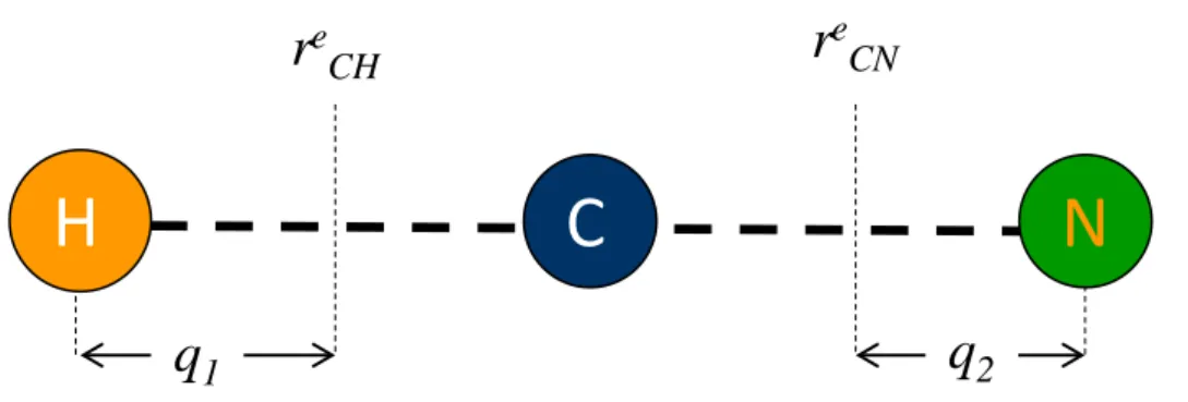
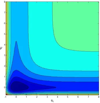
5.2 The HCN vibrational model . . . 53

6 HCN control results 57 6.1 HCN molecule without laser interaction . . . 57

6.1.1 Classical trajectories and Poincar´e surfaces of section . . 57

6.1.2 SALI indicator and diffusion coefficients . . . 62

6.2 HCN molecule interacting with laser . . . 62

6.2.1 SALI indicator . . . 64

6.2.2 Frequency map analysis . . . 66

6.2.3 Molecular dissociation and chaotic dynamics . . . 69

III

Control of dynamics on complex networks

75

7.2 Degree of a node . . . 81

7.3 Matricial description of networks . . . 81

7.4 Clustering measures . . . 83

7.5 Centrality measures . . . 84

7.5.1 Betweenness centrality . . . 84

7.5.2 Closeness centrality . . . 84

7.5.3 Eigenvector centrality . . . 85

7.6 Network models . . . 86

7.6.1 Random networks . . . 86

7.6.2 Small-world networks . . . 87

7.6.3 Scale-free networks . . . 89

7.7 Processes on networks . . . 91

7.7.1 Percolation and network resilience . . . 91

7.7.2 Consensus dynamics . . . 92

7.7.3 Synchronization on networks . . . 93

7.7.4 Spreading mechanisms . . . 95

7.7.5 Games on networks . . . 96

8 Game setup description 99 8.1 Consensus on networks . . . 100

CONTENTS xiii

8.1.2 Consensus based on neighbours’ average . . . 103

8.1.3 Transport and trade consensus . . . 104

9 Numerical game optimization 107 9.1 Genetic algorithms . . . 108

9.2 Optimal action based on GA . . . 109

10 Algebraic game optimization 113 10.1 Singular value decomposition . . . 113

10.2 Optimal action based on SVD . . . 117

10.3 Optimal design of team connections . . . 118

10.4 Different targeted subsets . . . 121

10.4.1 Single target subsets per team . . . 121

10.4.2 Multiple target subsets per team . . . 123

10.5 Competition games on target subsets . . . 125

IV

Conclusions

135

A.1.1 Symplectic Hamilton equations propagation . . . 141

A.1.2 SALI coefficient computation for HCN molecule . . . 142

Notation

The following list defines the mathematical notation used in the text:

R Real numbers field C Complex numbers field Rn Set of real vectors of size n Rm×n Set of real matrices of size m×n

A Matrix

Aij Matrix indexed for some purpose

AT The transpose matrix of the matrix A

A∗ The Hermitian conjugate of the matrix A

A−1 The inverse matrix of the matrix A

λ(A) An eigenvalue of the matrix A

σ(A) A singular vector of the matrix A

tr(A) Trace of the matrix A

kAkp induced p-norm of the matrix A

kAkF Frobenius norm of the matrix A

a Vector (column-vector)

aT Vector (row-vector) transpose of vector a

ai The ith element of the vector a

1 Column vector with all its entries = 1

diag(a) Diagonal matrix with diagonal entries equal to the elements of thea vector ˙

a Time derivative of vector a(= da/dt)

Df(x) Jacobian matrix of vector f

∇pH Gradient of the H scalar along vectorp

∇2H Hessian matrix of the H scalar

span(a) Subspace generated by the vectora

Chapter 1

Introduction

“The complexity of things - the things within things - just seems to be endless. I mean nothing is easy, nothing is simple.”

– Alice Munro “... No me atrevo a afirmar que son sencillos; no hay en la tierra una sola p´agina que lo sea, ya que todas postulan el universo, cuyo m´as notorio atributo es la complejidad.”

– Jorge Luis Borges, Cuentos completos The concept of complexity of a system can be addressed from different perspectives. As a quality of the system it refers to what makes the system complex, such as the presence of emergent properties as a consequence of the interactions within the different parts of the system. In its second meaning, complexity refers to the amount of information needed to describe the system [Est15]. For both points of view, complexity theory is a scientific discipline encompassing a wide range of concepts and phenomena which cannot be fully explained and analysed by traditional sciences and methodologies. Complex systems can display special properties such as spontaneous emergence, unpre-dictability and strong non-linearities, which yield distinctive effects on their behaviour. Complex systems theory includes ideas derived from a number of other disciplines such as physics, mathematics, computer science, information theory among others, and it covers such a wide spectrum of concepts as chaos theory, complex networks or nonlinear systems. The range of applications is very large: climatology, celestial mechanics, opinion trends on social networks, molecular dynamics, emergent phenomena and stock markets, to name a few. The modelling and analysis of the complex systems behaviour has experienced an improvement in the last decades due to the development of several math-ematical disciplines. In particular, two of the most commonly used are chaos theory and complex networks.

The concept of chaos is generally associated with randomness, but its math-ematical definition rather refers to deterministic (not random) systems whose behaviour is only predictable for a certain period of time. Said period depends on the nature of the problem under study, the available measurement accu-racy and the uncertainty that is acceptable for practical purposes: it ranges in the order of milliseconds (electric chaotic circuits) to millions of years (so-lar system). Indeed, the study of chaotic behaviour started with the classical mechanics description of the three-body problem, whose intricacies were ad-dressed by several scientists since Newton, with important contributions from Lagrange, Laplace, Hamilton, Jacobi, Weierstrass, etc., but it was only the French mathematician Henri Poincar´e who properly analysed the integrability of such systems in the XIX century [Poi1890]. Perturbation theory of Hamil-tonian systems is core for the understanding of chaotic behaviour. This topics was nicely addressed in the seminal work of Kolmogorov, Arnold, and Moser, in the middle of the 20th century [Kol54b] that provided an adequate setup for the analysis of chaos and the characterization of the transition from or-derly trajectories to chaotic ones as the amplitude of the perturbation of a Hamiltonian system is increased. As an output of such research they pro-duced the celebrated KAM theorem [Kol54a, Arn61, Mos68]. The study of dynamical chaos theory has substantially flourished thereupon, becoming an area of active research within the scientific community of dynamical systems [Ber78, Chi79, Gru00, Rad88, Lich92]. Furthermore, the interest in the field of chaos theory received an enormous boost since the 1960s after the advent of computers for analysis of practical scientific matters. Edward Lorenz was the pioneer in this line of research [Lor93]. While working on the study of weather prediction, he came across with chaotic behaviour when he decided to divide a simulation span in two parts, the second one starting with initial conditions based on the final output of the first one. The numerical accuracy in the defini-tion of those condidefini-tions for the second simuladefini-tion showed a completely different behaviour than the one observed without dividing the simulation in two. Such sensitivity to initial conditions is the trademark of chaotic systems, and its relevance in disciplines such as climatology, physical chemistry, physiology or fluid turbulence has been extensively studied ever since.

3 systems (gene regulatory networks, infection dynamics, species interaction), economics (bank lending mechanisms, market competitions, supply chains), telecommunications and electrical engineering (World Wide Web, power dis-tribution grids) or sociology (professional associations, political parties, clubs, and the like). The investigations conducted in numerous studies have proven that most social, biological, and technological networks are characterized by non-trivial topological features, with patterns of connection between their el-ements that are neither purely regular nor random. Besides the structural properties of complex networks, dynamical processes taking place on networks are also extremely important, such as the way traffic flows over the Internet or a disease spreads through a community. Scientific research on complex net-works has been mostly focused on topological properties of netnet-works and on the associated dynamics, while study of control techniques of such dynamics has basically started only in recent years.

As opposed to new developments on complex systems theory, the number of applications based on traditional physics had many years to develop and it is nowadays very extensively observed in all sort of daily technologies: internet, cell phones, air conditioning, terrestrial transportation, airplanes, television, etc. Numerous engineering applications have made use of the physics developed mostly during the XIX and 20th centuries for their routine use in modern life. Additionally, mathematics has experienced also an extraordinary development in parallel to physics during those decades, mutually impacting each other. One of the subjects strongly related to mathematics and physics is control theory. As described in the following lines, the purpose of this thesis is to contribute to the application of control (extensively used in technologies such as those listed in this paragraph) to complex systems, by providing relevant insights and conclusions on two problems studied here in depth.

Figure 1.1: Examples of centrifugal governor (left, [Por18]) and Jacquard’s loom (right [Ver17]).

the last decades the trend has been towards the use of software embedded in different sorts of central computing devices.

Two concepts are key in control theory: feedback and stability. The concept of feedback was present from the beginning as in the centrifugal governor's principle: two balls are connected to the rotary mechanism that is fed by a fuel valve. When the governor is at rest, the valve is open, while when it is rotating the balls rise due to the centrifugal force. This fact forces the central valve stem downward so that the valve gets closed, thus decreasing the rotation rate. This way, the engine is controlled to a constant speed by regulating the amount of admitted fuel, providing feedback to the system to compensate for variations in the load, external disturbances, etc.

5 of this theory.

After 1960, the methods and ideas used hitherto began to be considered as part of classical control theory. The new technology developments and appli-cations showed that models considered up to that moment were not accurate enough to describe the complexity of the real world. This generated important new efforts in this field and new techniques were found (mostly based on the time domain), including such substantial contributions as those obtained by R. Kalman in the filtering and estimation techniques [Kal60], or R. Bellman in the context of dynamic programming [Bry75]. For example, the Kalman filter was implemented in the Apollo program as a key algorithm to be used by the spacecrafts onboard navigation system on its way to the Moon [Grew10].

Besides the aforementioned concepts, optimization is another key topic in mathematics, engineering design and control. It can be regarded as a branch of mathematics whose goal is to maximize a benefit (or minimize a cost) by setting a number of variables to their most adequate value for such purpose. The underlying ideas are present in mathematical relevant topics such as the calculus of variations (the brachistochrone curve being a classical problem in this matter). Regarding control, one of the cornerstones of optimal control theory is the Pontryagin’s maximum principle [Bry75], which allows finding the best possible control for taking a dynamical system from one state to another in the presence of constraints. Its rationale is based on the maxi-mization of a Hamiltonian function (this function being also found in chaos theory as explained later on). Optimization theory is applicable to many prac-tical situations (power consumption minimization, shortest or quickest path, transportation routes design, etc.).

Control and estimation theory are currently areas of very intensive research in many subdisciplines: robust control, artificial intelligence, machine learning, etc. Their applications are ubiquitous in the automotive and aeronautical fields, cell phones, industrial automation, robotics, telecommunications, space engineering, etc.

of the game, the set information and actions available to each of them (and the strategies chosen based on those options), and the payoff for each player of the combined actions taken by him and his opponents.

From a control theory perspective, one can interpret a control law as a type of intelligent rational decision-maker designed to produce a desired effect. Ac-cordingly, game theory can be viewed as the study of conflict and cooperation between interacting controllers, where the identities and goals depend on the specific problem [Mar18]. For instance, the case of competition games con-siders two players where the benefit of one of them is obtained against the interests of the other. From a control point of view, the strategy followed by the opponent is considered by the other player as part of the environment and dynamics which the player is trying to control. Optimal control theory is also present in this setup, since the decision-making process followed by each player is defined to discern the best strategy against all possible decisions of the opponent. Furthermore, there is an important branch of control theory named robust control, in which the controller is designed based on a game theory setup using a minimax approach, where the external disturbance and noise are considered as opponent players against the robust controller, which chooses the optimal decision against all possible outcomes of disturbance and noise within a given range [Zho98].

A different game setting connected to control theory is that of cooperation games. In this subject, there can be many players and the defining feature is that all players follow decision dynamics ultimately leading to a given consen-sus. Generally, each player has access to different information, and thus it is not possible to follow a centralized controller implementation.

Therefore, game theory can be considered as a generalization of control theory. The second part of the thesis deals with both competition games and consensus dynamics.

As previously explained, the control theory is extensively developed in its application to linear systems [Oga10, Bay99]. Although to a lesser extent, stability and control theory for nonlinear systems has also the subject of deep research and application for many years. Important concepts in nonlinear control include perturbation theory and averaging, backstepping, sliding mode, etc. (see [Kha01] for a good review in the subject).

7 that one can lead a given chaotic system to follow a certain desired dynamic behaviour by means of properly chosen small perturbations, as opposed to non-chaotic systems for which the effort to attain this goal is typically on the order of magnitude of the unperturbed evolution of the dynamical variables. A relevant technique based on this idea is the OGY method (Ott, Grebogi, and Yorke, [Ott90]). This procedure is based on determining some of the unstable low-period periodic orbits that are implicit in the chaotic system dynamics, and based on the location and the stability of these orbits the control designer selects one which yields the desired system performance. Another example of control of chaotic systems is the topic of chaos synchronization, which has also been the subject of detailed study [Hea94, Boc02], and it is related also to communication systems by means of chaos. An extensive review of chaotic systems control is presented in [Boc00].

The first part of this thesis deals with the subject of control of Hamiltonian systems, and in particular the dynamics of the HCN molecule. It should be noted that one topic of paramount relevance in chemical dynamics is the active control of molecular dynamical systems and chemical reactivity. In the present research, the goal of the control is to characterize and select the actions that entail transition between regular and chaotic regime (and also on the molecule dissociation) depending on the value of the control parameter (namely the frequency of the laser exciting the molecule). In this thesis we have characterized the associated behaviour both in phase space and frequency domain, providing evidence of the underlying rationale associated to KAM theory. The research reported here was published in [Lop16].

more than one controller act on the dynamics of a certain system. The study of games on networks has been extensively explored in recent years from a number of perspectives [Nis07, Jack14, Bram14, Ell18, Kar11, Gal10, Ball06, Jack10]. The most commonly found framework features a number of agents linked by means of a complex network and following certain strategies, aiming to achieve a certain objective (i.e. maximizing an associated individual payoff). A typical example of this behaviour is given by the concepts of strategic complements and strategic substitutes, which constitute two canonical approaches for a va-riety of games [Jack14, Bram14, Gal10]. In many cases, the studied games deal with individuals’ behaviour within a social structure, as in [Ell18], where the decisions of single agents towards improvement of their payoff is studied, analysing the features of the network that lead to better Pareto equilibria. Social activities can also imply the search of a key player [Ball06]. A generic review of social and economic networks and associated games is presented in [Jack10]. In other cases, dynamics between biological agents are investigated, as in [Kar11] which addresses the competition of two diseases within a human population, aiming to maximize their spreading over the network.

Additionally, consensus dynamics in networks are also addressed in numer-ous papers in the literature. This concept includes such important phenom-ena as synchronization of coupled oscillators, as in the celebrated Kuramoto model [Kur84] where several elements connected through a complex network follow oscillatory dynamics which can lead to phase synchronism (and there-fore consensus) depending on the coupling gains. Another important consensus topic deals with flocks dynamics of mobile agents [Olf06] or robots coopera-tion [Ege02]. Other examples are related to consensus in small-world networks [Xia04] or information fusion algorithms for sensor networks [Xia05]. For a review of consensus dynamics, see [Olf07] and the references therein.

9 (GP) of elements is subject to certain consensus dynamics which depends on the nature of the real problem. Each competing team consists of a network of agents connected to GP, and each member of the team acts on the network with a certain intensity, influencing the consensus dynamics in order to max-imize the team’s payoff, while ensuring that the overall energy used by the team is bounded for the sake of competition fairness. The concept of energy is here associated to the effort exerted by each team on the game (e.g. money investment, resources dedication, etc.).

Moreover, this thesis considers several consensus dynamics among the mem-bers ofGP to reach a steady state, obtaining a theoretical optimal set of actions of the team’s members which takes into account such dynamics. Additionally, here we compare that result with numerical simulations obtained by genetic algorithms, verifying the optimal solution. The mathematical foundation re-lies on singular value decomposition aiming at maximum amplification in the desired singular vector. Furthermore, on this thesis we use the foundations set by this technique to establish the procedure for the optimal design of the con-nection between the elements of the team and the GP. As a result, one team is able to optimally connect with the general population so that its achiev-able performance is maximized against the other competing team which uses arbitrary connections.

The research presented here also analyses the possibility of each team aim-ing at some parts of the population, selectaim-ing its strategy and reactaim-ing to the action of the opponent team. The agents of each team are then divided in two or more subgroups, each of them specialized in targeting a certain subset of the general population. Thus, each team has the additional control variable of selecting how its action energy is distributed among those groups in order to maximize its payoff, taking into account the equivalent decision of the oppo-nent team. In this case one singular value is associated to each target group, and the optimum action selection is still based on the solution described in the thesis for the whole GP. Finally, it is shown that this setup defines cer-tain game dynamics. An application is considered at the end of the chapter including numerical simulation, where the associated strategies of both teams ultimately lead to a Nash equilibrium. This research has been presented in [Lop19].

Part I

Dynamics and Control

Chapter 2

Dynamical systems and chaos

theory

2.1

Dynamical systems

A dynamical system changes its state over time, defined by a number of vari-ables whose evolution is governed by a certain law, generally subject to external actions [Kat95, Hale91]. The rule for time evolution deterministically specifies how the state of the system, as given by a set of state variables, changes in time from a given initial condition (i.e. the initial state of the system). It is typi-cally defined by a state vector (i.e. position, velocity, etc.) contained within the state space (for example_Rn, withn the number of parameters defining it). Therefore, the three main concepts present in a dynamical system are:

• A state (or phase) space M which is associated to those features of the system that change over time.

• A time variable (either continuous or discrete) which is directly related to the unfolding of events.

• A time-evolution law. This is a rule that determines the state of the system at a given time as a function of the state in previous times. This implies also dependency of the dynamics on external actions, if applicable.

A dynamical system can be formally defined ([Bro10]) as a structure con-sisting of a state spaceM and an evolution operator:

φ :G×M →M

(t,x)7→φt(x) (2.1)

Here G is a semigroup (associated to the time) and x denotes the state vector of the dynamical system (each element in the vector representing one of the degrees of freedom of the system). The evolution operator satisfies the composition rule given by:

φt◦φs=φt+s (2.2)

IfG is a group, the dynamical system is invertible, resulting in the identity:

φt◦φt−1 =φ_e (2.3)

whereφt−1 denotes the inverse ofφ_tand withφ_ebeing the identity element. We refer to the set of phase space points followed by the time evolution of the systemφtas anorbit ortrajectory, starting from the initial conditionx0 ∈M.

There are two main types of dynamical systems depending on the nature of time:

• Continuous systems, with G = _R (for reversible systems) or G = _R+ (irreversible systems)

• Discrete systems, with G =_Z(reversible systems) or G =_N0(irreversible

systems)

The definition of reversibility is given at the end of this section, since it previously requires the concepts of vector field and map which are introduced in the following lines.

In this thesis both discrete and continuous dynamical systems are present. In particular, continuous Hamiltonian systems are studied in the first part of the thesis (vibrational dynamics of the HCN molecule). On the other hand, the second part deals with discrete dynamics over networks, in the form of consensus dynamics and games played over the network, both of which are described by a discrete time framework.

Let f ∈ C∞(M,_Rn) (with M ⊂ _Rn) be a function that implicitly defines the rule for the time evolution of an n-dimensional dynamical system by the initial value problem [Hale91]:

˙

x=f(x) andx(0) =x0 (2.4)

with x0 ∈ M being a given initial condition. Geometrically, the vector

2.1. DYNAMICAL SYSTEMS 15 are tangent to f at each point. Indeed, a solution is nothing but the orbit associated tox0. The family of solutions of possible phase space points Φ :Rn

x M →M is called theflow of the dynamical system.

A set U ⊆M is said to be invariant if, for every x∈U, φt(x)⊆ U for all

t. If a phase-space point is found such that φt(x) = xfor all t, xis said to be

a fixed point or equilibrium point. If, for a given x∈M, there is some T > 0 such that φT(x) = x, the minimumT for which this holds is called theperiod

of the closed orbit passing throughx. An orbit is calledperiodic if one point of the orbit is periodic, and hence all points are, as it follows by the composition rule that φt+T(x) =φT(x). Clearly, a periodic orbit is also an invariant set of

the dynamics.

A fixed point xe is said to be stable if for any given neighbourhood U(xe)

(i.e. any connected open set such thatxe∈U(xe)) there exists another

neigh-bourhoodV(xe) contained in it, V(xe)⊆U(xe), such that any solution

start-ing inV(xe) remains inU(xe) for allt ≥0. The set is said to beasymptotically

stable if it is stable, and if there is a neighborhood of xe such that for all xe

starting in it it holds that lim

t→∞kφt(x)−xek=0 (2.5) Fixed points can be analysed for both linear and non-linear systems. The dynamics of a linear system are given in general by means of the following equation:

˙

x=Ax (2.6)

where x ∈ _Rn _{is the state vector and A ∈}

Rn×n is the state or system

matrix. A broader definition including control inputs and sensor outputs is considered later in this chapter when studying control systems, by means of equation 3.8. The stability of a linear system can be studied by means of the eigenvalues of the matrix A [Bay99].

In the case of a non-linear system, a well known technique to characterize stability of fixed points is given by means of the so called Lyapunov functions [Kha01]. Nevertheless, a first approach to grasp the stability behaviour in the neighbourhood of a fixed point can be achieved by linearization of the system around the equilibrium by means of the Jacobian matrix of first partial derivatives of the vector fieldf:

˙

with x=xe+ξ, andξ ∈M a vector with kξk<<kxek

WhenDf(xe) has no eigenvalues with zero real part,xeis called ahyperbolic

equilibrium point. For this kind of points their stability type in the non-linear system is determined by the linearization process. This is not applicable for fixed points for which the eigenvalues of the Jacobian matrix have zero real parts. In order to characterize the stability of a hyperbolic fixed point of the non-linear system, we first remind that a homeomorphism is an one-to-one relation between points in two topological spaces that is continuous in both directions. Using this concept, an important theorem due to Hartman and Grobman [Guc83] states that for a hyperbolic fixed point xe there is a

home-omorphism h defined in some neighbourhood U of xe that locally associates

orbits of the nonlinear flowφt(x)⊆U to those of the linear flow etDf(xe).

We now define the local stable and unstable manifolds of xe in the

neigh-bourhoodU respectively as follows [Guc83]:

W_locs (x) ={xe∈U, φt(x)→xe as t→ ∞, and φt(xe)∈U ∀t≥0}

W_locu (x) ={xe∈U, φt(x)→xe as t→ −∞, and φt(xe)∈U ∀t≤0}

(2.8)

The global stable and unstable manifolds of xe are given by propagating

backwards in time the points in the local manifoldW_locs , and forwards for those in the local manifoldW_locu :

W_locs (x) = [

t≤0

φt(x)(Wlocs (x))

W_locu (x) = [

t≥0

φt(x)(Wlocu (x))

(2.9)

An orbit connecting one fixed point to itself is referred ashomoclinic. On the other hand, those trajectories that connect two distinct equilibrium points are namedheteroclinic. The closed path formed by heteroclinic orbits is called heteroclinic cycles.

2.1. DYNAMICAL SYSTEMS 17

x(n+ 1) =f(x(n)) (2.10)

where f : M → M is a map of the state space M into itself and (x(n)) denotes the state at the discrete time n. Each implementation of the math-ematical equations is called an iteration of the map. Area preserving maps provide the simplest and most accurate means to visualize and quantify the behaviour of conservative systems with two degrees of freedom. The logistic map is a classical scalar example (here M is given by _R), determined by a parameter λ >1 and defined as:

x(n+ 1) =f(λ, x(n)) =λx(n)(1−x(n)) (2.11)

The concepts of equilibrium points, stability and linearization described above for continuous systems are also applicable for discrete-time systems. The concepts of homoclinic and heteroclinic trajectories can also be applied for the Poincar´e map defined by the Surface of Section in §2.4.1. This is of high relevance when studying the presence of elliptic and hyperbolic points in the PSOS of dynamical systems, in particular the HCN dynamics under study in part II.

Before finishing this section, let us now define the concept of reversible dynamical system [Wig03]. We provide the definition for either a continuous or a discrete time dynamical system, which are respectively given by equations 2.4 and 2.10. We consider a map:

F :_Rn7→_Rn _(2.12)

such that:

F ◦F =φe (2.13)

where φe denotes the identity map. Thus F can be considered as an

invo-lution function. Then, a vector fieldf is said to be reversible if:

d(F(x))

dt =−f(F(x)) (2.14)

This can be described as the dynamics in the phase spaceF·_Rn_{being given}

DF ·x=−f ◦F (2.15)

Similarly, a map g is said to be reversible if

g(F(x(n+ 1))) =F(x(n)) (2.16) which implies that in the phase space F ·_Rn_{, the map g reverses the time}

direction of trajectories.

As a final remark, we should note that a dynamical system can be char-acterized by its behaviour in the time domain as described above (e.g. by means of differential equations in the continuous case or difference equations for discrete time systems) and also in the frequency domain (for example by means of transfer functions in the case of linear systems). This thesis mostly considers the time domain characterization, although frequency analysis is also used in some sections of part II, regarding dynamics of the HCN molecule.

2.2

Hamiltonian systems

One of the most fundamental description of dynamical systems is the formu-lation of physical phenomena in terms of the Lagrangian and Hamiltonian mechanics. The derivation of the Lagrange’s equation can be obtained based on the so called D’Alembert’s principle [Gol80]. For this purpose, we first define the virtual work of the ith force in the system Fi along the virtual

dis-placement δri by means of the dot product of these two vectors. Then, the

dynamics of the system are included into D’Alembert’s principle for systems where the virtual work of the forces of constraint vanishes. By introducing generalized coordinates qj in the equations (which are independent of each

other for holonomic constraints) the principle renders a preliminary form of Lagrange’s equations, withj = 1· · ·N andN being the number of coordinates:

d dt

∂T ∂q˙j

− ∂T

∂qj

=Qj (2.17)

where T is the kinematic energy and Qj denotes the generalized force

de-fined by:

Qj = N X

i=1

Fi·

∂ri

∂qj

2.2. HAMILTONIAN SYSTEMS 19 when the external forces can be derived from the gradient of a scalar po-tential functionV, equations 2.18 can be expressed in terms of the Lagrangian

L=T −V:

d dt

∂L

∂q˙j

− ∂L

∂qj

= 0 (2.19)

which are the classical form of Lagrange’s equations. It should be noted that this form of the equations can be used even if there is no potential function

V which depends only on the generalized coordinates, but there is instead a generalized potential U which depends also on the generalized velocities ˙qj,

and the Lagrangian is then given by L =T −U. A classical example of such systems is given by the Lorentz force which is applied when a charged particle moves in the presence of a magnetic field [Gol80].

Alternatively, the Lagrange’s equations can also be derived from Hamilton’s principle. If we define the line integral I of a system as the integral of the Lagrangian between two fixed times t1 and t2, this principle states that the

motion of the system is such that the variation of the line integral is zero:

δI =

Z t2

t1

L(q1,· · ·qN,q˙1,· · ·q˙N, t)dt = 0 (2.20)

An alternative description of the dynamics of a system is given in terms of Hamiltonian dynamics. According to Hamilton’s formulation, mechanical dynamical systems are described in terms of position coordinates and its con-jugate momenta, rather than of generalized velocities and positions as in the Lagrangian formulation. Hamilton’s equations are given by [Gol80, Fet80]:

˙

qi =

∂H

∂pi

˙

pi =−

∂H

∂qi

∂H

∂t =− ∂L

∂t i= 1, . . . , N (2.21)

where N is the number of degrees of freedom; and {qi} and {pi} are the

gen-eralized coordinates and their corresponding conjugate momenta, respectively. The vectorial form is expressed as follows:

dq

dt = ∂H

∂p,

dp

dt =− ∂H

∂q (2.22)

with (q,p) = (q1, q2, . . . , qN, p1, p2, . . . , pN) being the state vector formed

H and L respectively denote the Hamiltonian and Lagrangian functions describing the system, which are related by the Legendre transformation:

H(q, p, t) =

N X

i=1

( ˙qipi)− L(q,q˙, t) (2.23)

where ˙qi are the first derivatives of the generalized coordinates and pi =

∂L ∂q˙i

are defined as theith generalized or canonical momenta.

2.2.1

Phase space

The 2N dimensional space formed by the coordinates of the system {qi} and

their conjugate momenta {pi} is called the phase space of the system, as

op-posed to that formed only by the position coordinates, which is known as the configuration space. In phase space, each point represents a particular state of a dynamical system. The coordinates of the point are numerically equal to the values that the variables assume when the state occurs. Therefore, when these states of the system form a chain of points, this sequence represents the flow of the change of state of the dynamical system.

The motion of the system is obtained by integration of Eq. 2.21, starting from a suitable set of initial conditions,p(0), q(0). In this way, trajectories in phase space can be calculated as the evolution in time of this point (p(t),q(t)), where the motion of the system is most clearly visualized, since all dynamical information is readily apparent.

The Hamiltonian phase space has very special properties. If the system has some translational symmetry then some momenta may be conserved quantities [Fet80]. This concept is generalized in the Noether’s theorem [Noe1918].

Additionally, if the HamiltonianHdoes not depend upon time in an explicit way, then the system is also conservative, and it is defined as:

H =T +V(q) (2.24)

and represents the total energy of the system. For the general case, however, the Hamiltonian is not always conservative. For Hamiltonian systems there will be 2N dimensions forN degrees of freedom and chaos can occur only when N

2.2. HAMILTONIAN SYSTEMS 21 Phase space volume conservation

A volume element at some initial time, t0, can be written as

dV_tN₀ =dp1(t0)...dpN(t0)dq1(t0)...dqN(t0) (2.25)

It is related to a volume element,dVt, at timetby theJacobian,JN(t0, t) of the

transformation between phase space coordinates at time t0, {pi(t0)}, {qi(t0)}

and coordinates at time, t, {pi(t)},{qi(t)}. Thus

dV_tN =JN(t, t0)dVtN0 (2.26) For systems obeying Hamilton’s equations (even if they have a time dependent Hamiltonian), the Jacobian is a constant of the motion,

dJN(t, t0)

dt = 0 (2.27)

and therefore volume elements do not change in time. Thus the phase space behaves like an incompressible fluid.

On the other hand, dissipative systems are those for which phase-space volume contracts under the flow.

2.2.2

Conservative systems

The physical system that conserve total energy have always raised a special interest in the world of physics and mathematics. Often, a complicated sys-tem problem can be simplified to a conservative syssys-tem and enough insight obtained that the task of analysing the real system is made far easier. A system is considered conservative if the work to displace a particle between two arbitrary points is independent of the path followed between those two points. It can be shown that a necessary and sufficient condition for such re-sult is that the applied force can be derived from a scalar function of position. Thus, in a conservative system the potential energy, V, depends only on the position coordinates. For such systems the total energy E, remains constant with time and the classical mechanical Hamiltonian function turns out to be simply the total energy expressed in terms of position coordinates and con-jugate momenta. Conservation of energy in Hamiltonian mechanics requires that ∂H/∂t = 0. Then, the value of the Hamiltonian remains constant along any trajectory.

Integrable systems

In general, integrable systems have as many independent integrals of motion as they have degrees of freedom (Integrals of motion are also called constants of motion), and the corresponding dynamics is regular.

The mathematical condition for the conservation of a physical magnitude can be expressed by means of Poisson brackets 1.

Let us consider a phase space function,f(qi,pi, t)

df dt = ∂f ∂t + N X i=1 ∂f ∂qi ˙

qi+

∂f ∂pi ˙ pi (2.28) By using Hamilton equations, Eq. 2.28 can be rewritten as

df dt =

∂f

∂t +{f,H}Poisson (2.29)

where

{f,H}Poisson=

N X i=1 ∂f ∂qi ∂H ∂pi − ∂f ∂pi ∂H ∂qi (2.30) These relations can be used to express Hamilton’s equations as follows [Gol80]:

˙

qi ={qi,H}Poisson p˙i ={pi,H}Poisson (2.31)

It can be easily shown that the Poisson brackets fulfil

{f, g}Poisson=−{g, f}Poisson

and are invariant under canonical transformations2.

The conservation condition for a functionf(qi,pi,t) can then be expressed

in terms of Poisson brackets as:

1_{The Poisson bracket of two functions,r(q, p) ands(q, p), of the generalized coordinates}

and momenta,qj,pj, is defined as

{r, s}P oisson=

X j _∂r ∂qj ∂s ∂pj − ∂r ∂pj ∂s ∂qj

2_{Canonical transformation deal effectively with integrable systems. They corresponds to}

a transformation from one set of Hamiltonian coordinates (qA, pA) to another (qB, pB),

2.2. HAMILTONIAN SYSTEMS 23

{H, f}Poisson =

∂f

∂t (2.32)

Moreover, the integrability condition for a time independent conservative sys-tems can be expressed as

{fi, fj}= 0 (i, j = 1, . . . , N) (2.33)

where one of the conserved function is the Hamiltonian. Action–angle variable

Hamilton equations of motion can be written in terms of any convenient set of generalized coordinates. Therefore, one can transform between coordinate systems and leave the form of Hamilton’s equations invariant via canonical transformations. There is, however, one set of canonical coordinates which plays a distinctive role in terms of the analysis of chaotic behaviour in classical nonlinear systems. These are the action–angle variables [Fet80]. The systems in which motion is periodic are have a significant importance in physics. For the case of one degree of freedom, there are two types of periodic motion if we consider the evolution in the phase space.

1. In the first case, the orbit is closed and the system periodically revisits the same point in such space. This type of motion is referred aslibration

or also as a oscillatory motion.

2. The second type implies that the generalized momentum p periodically depends on the generalized coordinateq. This type of motion is generally defined as a rotation, and in this case q increases indefinitely (for a conservative system).

A classical example for one degree of freedom is the simple pendulum with mass m and longitude l. The Hamiltonian of the system is given by:

H(p, θ) =mgl(1−cos(θ)) + p

2

2ml2 (2.34)

which is equal to the total energy E. Here, θ denotes the angle of the pendulum with respect to the vertical direction and g is the gravity accelera-tion. When the energy of the system is below the maximum potential energy

E <2mgl, the motion follows an oscillatory pattern. The orbits have a stable equilibrium point for θ= 0, which is called an elliptic point. When E >2mgl

is a bifurcation point between both types of motion. It is an unstable equilib-rium point (hyperbolic) because all trajectories diverge from this point.

For either type of periodic motion we can define a new variable named action and defined in terms of the generalized coordinate and angular momen-tum:

I =

I

pdq (2.35)

In this equation, the integration is conducted over a complete period of the motion. Let us now consider a generic case of an integrable system. A canonical transformation from the old variables (p, q) to a new set of angle action variables, (I,θ), always exists, such thatHonly depends on the actions. Hamilton equations in these new coordinates present a specially simple form

˙

θi =

∂H

∂Ii

=ωi(I)

˙

Ii = −

∂H

∂θ˙i

= 0 (2.36)

that can be easily integrated giving

θi = ωi(I)t+δi

Ii = Ii0 (2.37)

whereωi are the N frequencies characterizing the motion.

For an integrable classical mechanical system with N degrees of freedom, each isolating integral of motion constrains flow of trajectories to a 2N − 1 dimensional surface in the 2N dimensional phase space. The actual flow of trajectories in phase space lies on the intersection of theseN surfaces. Thus, for integrable systems a given trajectory lies on anN dimensional surface (the interaction of N surfaces) in the 2N dimensional phase space and every tra-jectory is either quasiperiodic or periodic stable. This occur in n-dimensional tori 2.

2_{A two-dimensional torus is a surface of revolution generated by revolving a circle in}

three-dimensional space about an axis coplanar with the circle. Topologically, it corresponds to the product of two circles: T2 :S1×S1. An n-dimensional torus is a generalization given

2.3. DYNAMICAL CHAOS AND KAM THEORY 25

2.3

Dynamical chaos and KAM theory

2.3.1

Non–integrable classical systems. Chaos

As commented in the introduction, Henri Poincar´e was one of the first to discover the deterministic type of chaos. Edward Lorenz referred to chaos as physical processes that appear to proceed according to chance even though their behaviour is in fact determined by precise laws [Lor93].

Formally, chaos is defined in terms of the dynamical behaviour of pairs of orbits which initially are close together in phase space. If the orbits move apart exponentially in any direction in the phase space, the flow is said to be chaotic, which means that the flow defined by the dynamical system shows a sensitive dependence on initial conditions. A flow φt:A→A exhibits such dependence

if there is some δ > 0 such that for any x ∈ A and any neighbourhood U(x) there exists y∈A and t ≥0 so that

kφt(x)−φt(y)k> δ (2.38)

In order to determine the dependence of a dynamical system to initial conditions, the concept of Lyapunov exponents is commonly used [Sko10]. Lyapunov exponents are asymptotic measures of the average exponential rate of divergence of infinitesimally nearby initial conditions. Let us consider a dynamical system evolving on an N-dimensional phase-space manifold M and a connected region U → M. Let us further assume the dynamics of the continuous-time system to be represented by a system of first-order ODEs (see equation 2.4) starting from a given initial condition x0 ∈ U. Then, an

infinitesimal displacement along the trajectory represented by y(t) ∈ Tx(t)M

where Tx(t)M is the tangent (linear) space at the orbit point x(t), evolves

according to the following equation: ˙

y=Df(x)·y (2.39)

with Df(x) being the Jacobian matrix evaluated at x(t). The solution to 2.39 can be expressed by:

y(t) = Y(t,x)·y(0) (2.40)

where Y(t,x) is the fundamental matrix of solutions of equation 2.39. For ease of notation we will simply denoteY(t,x)·yasYt·y. Then, the Lyapunov

χ(x,y) = lim

t→∞sup 1

tlogkYt·yk (2.41)

It should be noted that the value of this exponent is independent of the norm kyk. If we rather considered the vector βy, where β is a real nonzero constant, then in the definition above there is an additional term log |β|/t, that in the limit goes to zero. Furthermore, the definition of this exponent is independent of the type of vector norm.

Let us consider now a set of p linearly independent vectors in_Rn, denoted by yi, with i = 1,2,· · · , p Ep the subspace generated by this set of vectors

andvolp(Yt, Ep) the volume of the parallelogram of dimension p with edges the

vectorsYt·yi, computed as the norm of the wedge product of these vectors:

volp(Yt, Ep) = kYt·y1∧Yt·y2∧ · · · ∧Yt·ypk (2.42)

We define the LCE of order p of Yt with respect to Ep as

χ(Yt, Ep) = lim t→∞sup

1

tlog volp(Yt, E

p_{) (2.43)}

There will be one such exponent for each dimension phase space, and they are referred as the Lyapunov spectrum. Typically, the largest Lyapunov expo-nent is called the maximum Lyapunov expoexpo-nent. These expoexpo-nents are used to determine the nature of the dynamics of the system. If all the Lyapunov expo-nents are zero, the dynamical flow is regular. If just one exponent is positive, the flow will be chaotic.

As stated before, a system withN degrees of freedom is integrable if it has

N independent isolating integrals. In the same way, the systems which do not fulfil this condition are said to be non–integrable or chaotic.

Non–integrable systems may themselves be divided into two classes. One class contains the completely chaotic systems such as the Sinai billiard and the non–circular stadium. Such systems generally have infinite hard convex surfaces or hard surfaces and irregular shape. The hard surface makes the Hamiltonian non–smooth. They contain an infinite number of periodic orbits but they are all unstable. Non–integrable systems with smooth Hamiltonians comprise the second class of non–integrable system.

2.3. DYNAMICAL CHAOS AND KAM THEORY 27

Figure 2.1: Graphical representation of phase space foliated by tori. (Adapted from [Sco14])

orbits and chaotic orbits, and a mixture of stable and unstable periodic orbits. Although the motion of these systems is not restricted to tori, it can in general be very complicated. Chaotic regions occur when isolating integrals of motion are destroyed locally by nonlinear resonances.

2.3.2

KAM and Poincar´

e–Birkhoff Theorems

Between the two extreme cases of the behaviour of the dynamical system, integrable and completely ergodic, there are many intermediate cases. Some of invariant tori, resonant tori, which affected by the perturbation will be destroyed, meanwhile the non–resonant ones resist to destroy and continue as invariant tori. The non–resonant tori which have not been destroyed by resonances are called KAM tori or KAM surfaces 3. The KAM theory applies to a generic Hamiltonian system whose motion is governed by a Hamiltonian of the form

H=H0+εH1 (2.44)

where ε is a small parameter controlling the degree of the perturbation. The zeroth–order Hamiltonian,H0, is an integrable approximation toH, which has

nonzero Hessian andH1 is the perturbation term which for oscillator systems

can be written in terms of action–angle variable as [Chi79]:

H1 =

∞

X

n1=−∞ ∞

X

n2=−∞

Vn1,n2(I1, I2)e

i(n1θ1+n2θ2) _(2.45) 3_{A resonant torus in the phase space has an associated frequency vector ω such that}

there is a vector k∈_Zn _{(except the vector 0) such that k·ω=0. If no suchkexits, the}

The KAM theorem (due to Kolmogorov, Arnold and Moser) demonstrates the continued existence of certain invariant tori as the perturbation parameter

ε increases from 0, at which the system is considered to be integrable. When

ε 6= 0 the system moves to non–integrability, but in a way which is explained by this theorem. The tori which are characterized by a ”sufficiently irrational” frequency ratio, α = ω1/ω2, survive. Such ratio is also referred as winding

number. For a two degrees of freedom system this irrationality condition is given by ω1 ω2 − n m

> K(ε)

m5/2 (2.46)

for all integer numbersn andm. K(ε) is a function of the perturbation which tends to zero as the perturbation disappears. These tori, which are only dis-torted by the perturbation, are calledKAM tori. The rest of tori are destroyed, but according to two different mechanisms depending on the value of α (see figure 2.2).

If α is a rational number (resonant tori), the previous condition does not hold for any value of the perturbation. The fate of these tori is regulated by the Poincar´e–Birkhoff theorem [Losk07, LeC10], which states that: under small enough perturbations, an even number of fixed points of the original torus survive; half of them are elliptic, and the other half are hyperbolic. The elliptic points are surrounded by new tori (stability islands), some of them rational, and some of them irrational. Again the rationals and some of irrationals will be destroyed by the perturbation, according to the KAM theorem. Then, the previous structure is repeated again and again at a finer scale.

In the neighbourhood of the hyperbolic points (related to the separatrix of H0) the motion becomes very complex, due to the homoclinic oscillations

discovered by Poincar´e. The incoming and outcoming manifolds cannot cross, and then they cross to themselves an infinite number of times. The points at which they cross are referred as homoclinic, and they form the so called homo-clinic tangle (see figure 2.3). These tangles constitute bands of stochasticity or chaos, which are separated from each other by the intact KAM tori [Chi79]. Rational approximates

2.3. DYNAMICAL CHAOS AND KAM THEORY 29

Figure 2.2: Destruction of tori. Source: [Losk07]

of a continued fraction as follow:

w≡[a0, a1, a2, ...] =a0 +

1

a1+ _a 1

2+_a 1 3+...

(2.47)

with ai integer and ai ≥1 for i≥1. Each rational and irrational number may

be represented uniquely by a sequence [a0,a1, ...]. For irrational numbers the

sequence will contain an infinite number of entries. The rational approximates to a given continued fraction are obtained by terminating the sequence by letting ai = ∞. Thus, for a given sequence, w = [a0, a1, a2, ...], the rational

approximatesNi/Mi, are given by

Ni

Mi

= [a0, a1, ..., ai,∞] (2.48)

The most ”irrational number” is given by the sequence ai = 1 for all i. That

is

[1,1,1, ...,1, ...]≡γ = 1 2(1 +

√

5) (2.49)

Figure 2.3: Graphical representation of the Poincar´e Homoclinic tangles, adapted from [Wig03]

It is well known that the KAM tori are destroyed by resonances between degrees of freedom whose periods are rationally related. Thus, each rational approximate will be associated to a resonance region in the phase space and a corresponding island chain. Furthermore, the last KAM torus that is destroyed has an winding number equal to the aforementioned golden mean.

Cantori

2.4. CHAOS INDICATORS 31 structure in it.

Systems with more than two degrees of freedom

For systems with two degree of freedom, the existence of invariant tori has a drastic effect in the structure of the phase space. Since two trajectories cannot cross in phase space, each cantorus divide it into two unconnected parts. However, for systems withN > 2 this is not true: a hypersurface ofN

dimensions (corresponding to an invariant torus of a N–dimensional system) do not define an inner and an outer regions in a space of 2N - 1 dimensions (energy shell).

Then, despite the existence of zones of regular motion, the chaotic areas are interconnected, constituting what is known as the Arnold web, and a single trajectory can explore the whole chaotic region, giving rise to what is known as Arnold diffusion.

2.4

Chaos indicators

There are several indicators that can be used for the characterization of the dynamics of Hamiltonian systems, The most popular one is the Poincar´e Sur-face of Section (PSOS) which has the limitation of being applicable only to 2D dynamical systems. This chapter describes this method along with the SALI coefficient and the Frequency Analysis indicator.

2.4.1

Poincar´

e surface of section (PSOS)

A very convenient way to distinguish between regular (non–chaotic) behaviour and chaotic motion is by looking at a diagram called a Poincar´e surface of section (PSOS), which is used to visualize the structure of phase space in dynamical systems with two degrees of freedom. The PSOS is a representation of the intersection of a given trajectory with a suitable plane in phase space, taking only those points for which the plane is crossed in a given direction.

The PSOS defined in this way consists of a sequence of points (p1(0), q1(0))

T

−→ (p1(1), q1(1))

(p1(1), q1(1))

T

−→ (p1(2), q1(2))

. . . (2.50)

Figure 2.4: Graphical representation of the Poincar´e Surface of Section. In order to visualize the PSOS, let us consider a conservative system. The Hamiltonian of a conservative system is the isolating integral of the motion and can be written as

H(q1, q2, p1, p2) =E (2.51)

where the energy, E, is constant and restricts trajectories to lie on a three dimension surface embedded in the four dimension of phase space. So that, one can express one of the variables as a function of the others. For example, let us take p2 as

p2 =p2(q1, q2, p1, E) (2.52)

It is evident from Eq. 2.52 that p2 depends parametrically on the energy,

E. For a certain energy level E, the trajectory is limited to a 3D volume (q1, q2, p1), and furthermore, a planeq2 = constant may be sequentially crossed

by the system trajectory [Lich92]. In general, the intersections of the trajectory which this plane can occur anywhere within a certain area of the plane.

If additionally the system has a second isolating integral,

I(q1, q2, p1, E) = I0(=constant) (2.53)

then equation 2.53 can be used for obtaining

2.4. CHAOS INDICATORS 33 The combination of Eq. 2.53 and Eq. 2.54 gives

p1 =p1(q1, q2, E, I0) (2.55)

Ifq2 = 0, then the trajectory lies on a one dimensional curve. This fact can be

used to determine the existence of constants of motion. By the construction of the PSOS, it will be easy to distinguish between the motion in the regular regime and the motion in the ergodic regime. The motion in the regular regime takes place on the surface of a torus, which renders a line in the PSOS when it is cut by the sectioning plane. On the other hand, in the ergodic regime, the motion takes place in the 3D energy shell, and then the successive intersections of the trajectory with the PSOS will fill in an area.

Another important property of the PSOS is that it allows to observe the appearance of chains of islands. When chaos is present in Hamiltonian systems, it is observed that regular motion and chaos regions coexist for any energy, and that the proportion of chaos increases with energy. This behaviour is general for any typical Hamiltonian system and can be explained with the aid of the previously described KAM and Poincar´e – Birkhoff theorems.

The global structure of the phase space can be visualized by composite PSOS, which consists in the superposition, in the same figure, of the PSOS of a significant ensemble of trajectories calculated with different initial conditions, all of them calculated at the same energy.

The concept of a surface of section can be generalized to systems with N >

2 degrees of freedom. For a time-independent Hamiltonian with N degrees of freedom, the energy surface in phase space has dimensionality 2N−1 [Lich92]. As in the case of two degrees of freedom (for example pN), we project one

generalized coordinate and then consider the intersection of the orbit with the 2N−2 surface of section defined byqN =constant. In this case, if the motion

is approximately separable for each degree of freedom, the N −1 projections of this multidimensional surface of section onto the (pi,qi) planes can be used

to visualize the evolution of the trajectory. Thus, in this case one plot is not enough to evaluate the dynamics of the system as in the case of two degrees of freedom, and one has to resort to the use of several graphs for such purpose.

2.4.2

The SALI coefficient

) (1 2 t z ) (1 2 t vr ) (1 1 t

z

z

(

t

)

r

v ) 0 ( 1 z ) 0 ( 1 vr ) 0 ( 2 vr ) 0 ( ˆ1 v ) 0 ( 2 z ) ( ˆ2 t1

v ) (1 1 t vr

)

(

t

z

r

)

(

t

z

r

Figure 2.5: Graphical illustration of the calculation of the SALI indicator [Lop16].

vectors. It is calculated from the integration of Eqs. (2.21), and its applicability is essentially independent of the dimensionality of the system.

Let us consider a reference trajectory, defined by the system state (column) vector

z= (q,p)∗ (2.56)

where the asterisk denotes the transpose operation. Hamilton equations of motion for this variable are written in symplectic form as

dz

dt =J

∂H(z)

∂z =J ∇H(z) (2.57)

with

J =

0N IN

−IN 0N

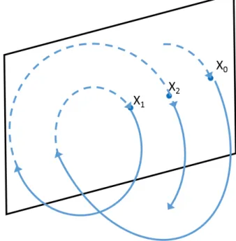
(2.58) Let us consider now two nearby trajectories,z1 andz2, as shown in Figure 2.5.

The evolution of the deviation vectorsvi =z−zi (i= 1,2) is given as

d(z−vi)