Fuzzy Controller for UAV-landing task using 3D-position Visual
Estimation
Miguel A. Olivares-M´endez
Student Member, IEEE
, Iv´an F. Mondrag´on
Pascual Campoy
Member, IEEE
and Carol Mart´ınez
Student Member, IEEE
Abstract—This paper presents a Fuzzy Control application
for a landing task of an Unmanned Aerial Vehicle, using the 3D-position estimation based on visual tracking of piecewise planar objects. This application allows the UAV to land on scenarios in which it is only possible to use visual information to obtain the position of the vehicle. The use of the homography allows a realtime estimation of the UAV’s pose with respect to an helipad using a monocular camera. Fuzzy Logic allows the definition of a model-free control system of the UAV. The Fuzzy controller analyzes the visual information to generate altitude commands for the UAV in a landing task.
I. INTRODUCTION
The unmanned aerial vehicle (UAV) has made its way quickly and decisively to the forefront of current aviation technology. Opportunities exist in a broadening number of fields for the application of UAV systems as the components of these systems become increasingly lighter and more powerful. Of particular interest are those occupations that require the execution of missions which depend heavily on dull, dirty, or dangerous work, UAVs provide a cheap, safe alternative to manned systems and often provide a far greater magnitude of capability.
Computer vision has played and important role on the growing development of UAV, in which has been used as an important sensor, initially used for surveillance and then being integrated on the control system of the vehicle in order to use the rich information provided by visual systems as the main source of information for a vast list of applications, covering from visual control system based on regular cameras [13], [1] to autonomous landing [7], [19] and obstacle avoidance [10], [2].
In contrast to conventional control, fuzzy control was initially introduced as a model-free control design method based on a representation of the knowledge and the reasoning process of a human operator. Fuzzy logic can capture the continuous nature of human decision processes and as such is a definite improvement over methods based on binary logic (which are widely used in industrial controllers). Hence, it is not surprising that practical applications of fuzzy control started to appear very quickly after the method had been introduced in publications. Some of those applications of Fuzzy control and UAV are: for visual servoing [18], for an autopilot using a Fuzzy PID control [20], an obstacle avoidance and path planning system [8] and to manage a team of UAVs [25].
All the authors belong to the Computer Vision Group, Universidad Polit´ecnica de Madrid, ETSII, Madrid - 28006 Spain (Email: [email protected])
Our research interest focuses on developing computer vision techniques to provide UAVs with an additional source of information to perform visually guided task - this includes tracking and visual servoing, inspection, autonomous landing and positioning, or ground-air cooperation. These situations need reliable state information, that allows a onboard con-troller to generate accurate positioning. In general the pose information is estimated based on the the GPS and the inertial measurement unit IMU sensor measurements. However, for low altitude tasks in urban scenarios, the estimation often is inaccurate because it is affected by GPS dropouts, thus making flying in these constrained environments more vul-nerable and more prone to problems. Computer vision as passive sensor not only offers a rich source of information for navigational purposes, but it can be also used as a main navigational sensor in place of GPS. With the increasing interest in UAVs, a visual system that can determine the robot 3D location in its operational environment is becoming a key sensor for civil applications.
This paper presents a Fuzzy Controller which use the visual information obtained by a real time 3D-position es-timation method, based on the tracking of a helipad using robust homographies estimation for descend in landing tasks. Section II explains the visual algorithm used in order to robustly track the reference landmark or helipad. Section III explains how the pose of a planar object relative to a moving camera coordinate center is obtained, using frame-to-frame homographies and the projective transformation of the reference object on the image plane. The definition of the Fuzzy controller used to analyze the visual information estimated onboard the UAV is presented in Section IV. Finally, Section V shows the specifications of the Unmanned Helicopter, and the test results of the proposed algorithm running onboard a UAV, by comparing the estimated 3D pose data with the one given by the inertial Measurement Unit IMU. This validates our approach for an autonomous landing control based in visual information.
II. VISUALPROCESSING
used to to obtain the 3D pose of the object with respect to the camera coordinate system.
On images with high motion, good matched features can be obtained using the well know Pyramidal Lucas-Kanade algorithm modification [12]. It is used to solve the problem that arise when large and non-coherent motion are present between consecutive frames, by first tracking features over large spatial scales on the pyramid image, obtaining an initial motion estimation, and then refining it by down sampling the levels of the images pyramid until it arrives at the original scale.
The set of corresponding or matched points between two consecutive images ((xi,yi)↔(x0i,y
0
i)fori=1. . .n,) obtained using the pyramidal Lucas-Kanade optical flow is used to compute the 3x3 matrix H that takes each ¯xi to ¯x0i or ¯x0i=H¯xi or the Homography that relates both images. The matched points often have two error sources. The first one is the measurement of the point position, which follows a Gaussian distribution. The second one is the outliers to the Gaussian error distribution, which are the mismatched points given by the selected algorithm. These outliers can severely disturb the estimated homography, and consequently alter any measurement based on homographies. In order to select a set of inliers from the total set of correspondences so that the homography can be estimated employing only the set of pairs considered as inliers,robust estimation using Random Sample Consensus (RANSAC) algorithm [9] is used. It achieves its goal by iteratively selecting a random subset of the original data points by testing it to obtain the model and evaluating the model consensus, which is the total number of original data points that best fit the model. In the case of a Homography, four correspondences are enough to have a exact solution or minimal solution using the Inhomogeneous method [6]. This procedure is then repeated a fixed number of times, each time producing either a model which is rejected because too few points are classified as inliers, or a refined model. When total trials are reached, the algorithm returns the Homography with the largest number of inliers.
III. 3DESTIMATION BASED ONHOMOGRAPHIES
This section shows how to estimate the 3D position of a world plane relative to the camera projection center for every image sequence using previous frame-to-frame homo-graphies and the projective transformation at first, obtaining for each new image, the camera rotation matrix R and a translational vector t. This method is similar to the one propose by Simon et. al.[24], [23] and is deeply detail on [14].
A. World plane projection onto the Image plane
Mondragon2010ICRA In order to align the planar object on the world space and the camera axis system, we consider the general pinhole camera model and the homogeneous camera projection matrix, that maps a world point xw inP3
to a point xi on ith image in
P2, defined by equation 1:
sxi=Pixw=K[Ri|ti]xw=K ri
1 ri2 ri3 ti
xw (1)
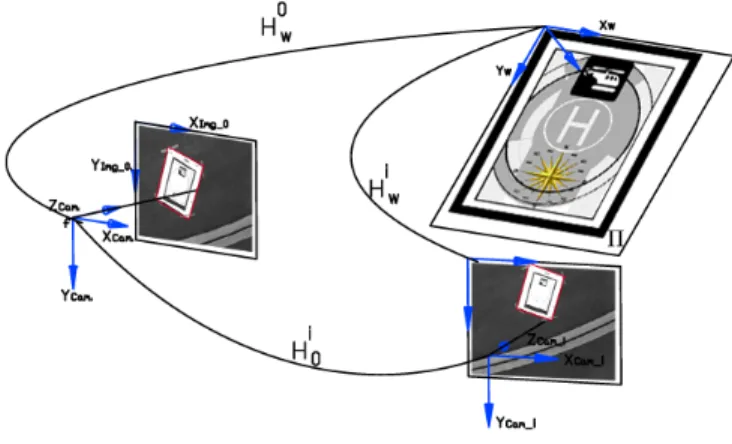
where the matrix K is the camera calibration matrix, Ri and ti are the rotation and translation that relates the world coordinate system and camera coordinate system, and s is an arbitrary scale factor. Figure 1 shows the relation between a world reference plane and two images taken by a moving camera, showing the homography induced by a plane between these two frames.
Fig. 1. Projection model on a moving camera and frame-to-frame
homography induced by a plane.
If point xw is restricted to lie on a plane Π , with a
coordinate system selected in such a way that the plane equation of Π is Z=0, the camera projection matrix can
be written as equation 2:
sxi=PixΠ=P
i
X Y 0 1
=hPii
X Y 1
(2)
wherehPiidenotes that this matrix is deprived on its third column or hPii=Kri1 ri2 ti. The deprived camera pro-jection matrix is a 3×3 projection matrix, which transforms points on the world plane ( now inP2) to theith image plane
(likewise inP2), that is none other that a planar homography Hi
w defined up to scale factor as equation 3 shows.
Hiw=K ri
1 ri2 ti
=hPii (3)
Equation 3 defines the homography which transforms points on the world plate to theithimage plane. Any point on the world plane xΠ= [xΠ,yΠ,1]T is projected on the image
plane as x= [x,y,1]T. Because the world plane coordinates system is not know for theith image,Hi
w can not be directly evaluated. However, if the position of the word plane for a reference image is known, a homographyH0
w, can be defined. Then, theithimage can be related with the reference image to obtain the homographyHi
0. This mapping is obtained using
sequential frame-to-frame homographiesHi
i−1, calculated for
any pair of frames (i-1,i) and used to relate theith frame to the first image Hi
0using equation 4:
This mapping and the aligning between initial frame to world plane reference is used to obtain the projection between the world plane and the ith image Hiw=Hi0H0w. In order to relate the world plane and the ith image, we must know the homography H0w. A simple method to obtain it, requires to match four points on the image with the corresponding corners of the rectangle in the scene, forming the matched points (0,0)↔(x1,y1), (0,ΠWidth)↔(x2,y2),
(ΠLenght,0)↔(x3,y3)and(ΠLenght,ΠWidth)↔(x4,y4). This
process can be done by both, a helipad frame and corners detector or by an operator through a ground station interface. The helipad points selection generates a world plane defined in a coordinate frame in which the plane equation of Π
is Z =0. With these four correspondences between the world plane and the image plane, the minimal solution for homography H0w=
h10w h20w h30w
is obtained.
B. Translation Vector and Rotation Matrix
The rotation matrix and the translation vector are com-puted from the plane to image homography using the method described in [28].
From equation 3 and defining the scale factorλ=1/s, we have that
r1 r2 t
=λK−1Hiw=λK−1h1 h2 h3 where
r1=λK−1h1, r2=λK−1h2, t=λK−1h3
(5)
The scale factor is calculated asλ =kK−11h
1k .
Because the columns of the rotation matrix must be orthonormal, the third vector of the rotation matrixr3could
be determined by the cross product ofr1×r2. However, the
noise on the homography estimation causes that the resulting matrixR=r1 r2 r3
does not satisfy the orthonormality condition and we must find a new rotation matrixR0that best approximates to the given matrix R according to smallest Frobenius norm for matrices (the root of the sum of squared matrix coefficients) [26] [28]. As demonstrated by [28], this problem can be solved by forming the Rotation Matrix R=
r1 r2 (r1×r2)=USVT and using singular value
decomposition (SVD) to form the new optimal rotation matrixR0=UVT.
The solution for the camera pose problem is defined as xi=PiX=K[R0|t]X. The translational vector obtained is
already scaled based on the dimensions defined for the reference plane during the alignment between the helipad and image I0, so if the dimensions of the world rectangle
are defined in mm, the resulting vector tiw= [x,y,z]t is also in mm. In [14], it is show how the Rotation Matrix can be decomposed in order to obtain the Tait-Bryan or Cardan Angles, which is one of the preferred rotation sequences in flight and vehicle dynamics. Specifically, these angles are formed by the sequence: (1 )ψ aboutzaxis (yawRz,ψ), (2) θ about ya (pitch Ry,θ), and (3) φ about the final xb axis (rollRx,φ), wherea andb denote the second and third stage in a three-stage sequence or axes.
C. Estimation Filtering.
An extended Kalman Filter (EKF) has been incorporated in the 3D pose estimation algorithm in order to smooth the position and correct the errors caused by the homography drift along time. The state vector is defined as the position [xk,yk,zk] and velocity [∆xk,∆yk,∆zk] of the kth helipad
expressed in the onboard camera coordinate system. We consider the dynamic model as a linear system where system has constant velocity, as presented in the following equations:
xk=Fxk−1+wk (6)
xk yk zk ∆xk ∆yk ∆zk
=
1 0 0 ∆t 0 0
0 1 0 0 ∆t 0
0 0 1 0 0 ∆t
0 0 0 1 0 0
0 0 0 0 1 0
0 0 0 0 0 1
xk−1
yk−1
zk−1 ∆xk−1 ∆yk−1 ∆zk−1
+wt−1
(7) Where xk−1 is the state vector (position and velocity), F
is the system matrix,wthe process noise, and∆t represents
the time step.
Because the visual system only estimates the position of the helipad, the measurements are expressed as follows:
zk=
¯ xk ¯ yk ¯ zk
+vk (8)
Wherezk is the measurement vector and[x¯k, ¯yk,¯zk]t is the
position of the helipad with respect to the camera coordinate system andvkis measurement noise . With the previous
defi-nitions, the two phases of the filter Prediction and Correction can be formulated as presented in [27], assuming that the process noise wk and the measurement noise vk are white,
zero-mean, Gaussian noise with covariance matrixQandR, respectively.
The output of the filter is the smoothed position of the helipad, that will be used as input for the control system.
IV. FUZZYCONTROLLERSYSTEM
This Section presents the implementation of the Mamdani Fuzzy controller which analyzes the visual information in order to generate descend commands for the UAV (velocity commands in meters per seconds).
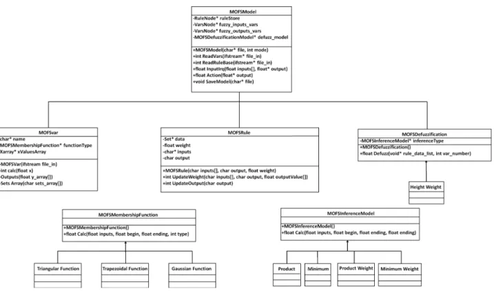
Fig. 2. Classes structure of the Miguel Olivares’ Fuzzy Software.
the defuzzification phase the Height weight method is used (Eq. 9).
y=∑
M
l=1yl∏ µB0(yl)
∑Ml=1∏ µB0(y¯l)
(9)
.
Additionally, the four subtypes of inference models for the fuzzification that have been implemented are the maximum and the product with and without taking into account the rule-weight characteristic of each rule. The weight of each rule is a part of a learning algorithm based on the idea of the synaptic weights of the neurons, but for this work this improvement is not used, in [17] and [16] is possible to see how it works. With this learning algorithm is possible to adapt the base of rules to a particular behavior, by reading patterns of inputs and its corresponding correct output.
More details about the structure of this software can be found in [15].
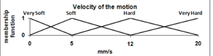
The controller is implemented for control the altitude of the UAV in order to be capable to made an auto-landing. This controller is working inside the vision-computer, that is onboard the UAV. Are defined two inputs and one output for the fuzzy controller. For the definition of the variables an heuristic method is used. The data is acquired from different manual and hover flight tests. The two inputs are: the estimation of the altitude, that is made by the homography (Fig. 3), and the variation of this value between the last two frames (Fig. 4). For this last input is taking into account possible variation of the frame-rate of the camera in the last second, in order to keep it more robust for possible changes
of the frame-rate caused by some computer operations. The output of the controller is the velocity command to send to aircraft to approximate to the helipad location (Fig. 5).
The control is made based on camera configuration, like a eye-to-hand configuration, because the camera is fixed on the UAV. The position of the camera respect the robot, the configuration of the system is an eye-in-hand type, and talking about the architecture of the visual and servo system, the implementation is based on a dynamic look-and-move visual control, that sends commands on velocity, because the 3D pose is estimated using the homography, taking into account the characteristic of the helipad and the intrinsic parameters of the camera, and, then, the controller sends velocity commands to move the UAV.
Fig. 3. Estimation of the altitude (in mm), based on the homography
of the helipad.
V. TESTS ANDRESULTS
This section shows the specification of the UAV, and the landing and pose estimation tests.
Fig. 4. Velocity of the position changes (in mm/s), tacking into account the estimation of the homography and the frame-rate of each moment.
Fig. 5. Output of the Fuzzy Controller, the velocity commands for
the UAV in m/s
an Xscale-based flight computer augmented with sensors (GPS, IMU, Magnetometer, fused with a Kalman filter for state estimation). Additionally they include a pan and tilt servo-controlled platform for many different cameras and sensors. In order to enable it to perform vision processing, it also has a VIA mini-ITX 1.5 GHz onboard computer with 2 Gb RAM, a wireless interface, and support for many Firewire cameras including Mono (BW), RAW Bayer, color, and stereo heads.
Fig. 6. COLIBRI III Electric helicopter UAV used for pose estimation
tests.
The system runs in a client-server architecture using TCP/UDP messages. The computers run Linux OS working in a multi-client wireless 802.11g ad-hoc network, allowing the integration of vision systems and visual tasks with flight control. This architecture allows embedded applications to run onboard the autonomous helicopter while it interacts with external processes through a high level switching layer. The visual control system and additional external processes are also integrated with the flight control through this layer using TCP/UDP messages, forming adynamic look-and-move[11] servoing architecture as is explained on Section IV and is shown in figure 7. The helicopter’s low-level controller is based on PID control loops to ensure its stability. Because features are extracted in the image and then used to estimate the pose of the helipad or target with respect to the camera coordinate system (fixed on the UAV camera platform), our control scheme is considered to be Position Base Visual Servoing (PBVS) system [11], [4], [22]. In this kind of control, an error between the current and the desired pose of
Fig. 7. UAV onboard visual control system following adynamic
look-and-movearchitecture
the camera-UAV is calculated and used by a fuzzy controller to generate the velocity references used by the low level controller to descend the UAV.
For these test a Monocromo CCD Firewire camera with a resolution of 640x480 pixels is used. The camera is calibrated before each test, so the intrinsic parameters are know. The camera is installed in such a way that it is looking downward with relation to the UAV. A known rectangular helipad is used as the reference object to which estimate the UAV 3D position. It is aligned in such a way that its axes are parallel to the local plane North East axes. This helipad was designed in such a way that it produces many distinctive corners for the visual tracking. Figure 8, shows the helipad used and the coordinate systems involved in the pose estimation. For
Fig. 8. Helipad, camera and U.A.V coordinate systems
these tests a series of landing flights in autonomous mode at different heights were done. Figure 9 shows the first frame for tree different test. The test begins when the UAV is hovering over the helipad. Then a user (through the ground station interface) manually selects four point on the image that corresponds to four corners on the helipad, forming the matched points (0,0)↔(x1,y1),(910mm,0)↔(x2,y2),
(0,1190mm)↔(x3,y3) and (910mm,1190mm)↔(x4,y4).
coordinates frame in which the plane equation ofΠisZ=0
and also defining the scale for the 3D results. With these four correspondences between the world plane and the image plane, the minimal solution for homographyH0w is obtained. Then, the UAV is moved, making changes on Z axis, (X,Y axes are controlled by the autopilot, maintaining a hovering condition while the helicopter is descending ). The helipad is constantly tracking by estimating the frame-to-frame homo-graphiesHii−1, which is used to obtain the homographiesHi0, andHiw from which Riw andtiw is estimated. The 3D poses estimation process is done with an average of 12 frames per second FPS.
Fig. 9. Helipad position on each of the different landing tests. The helipad
is oriented in such a way that theXaxis is the North position, theY axis
is the East position andZaxis is the Down Position (Earth center).
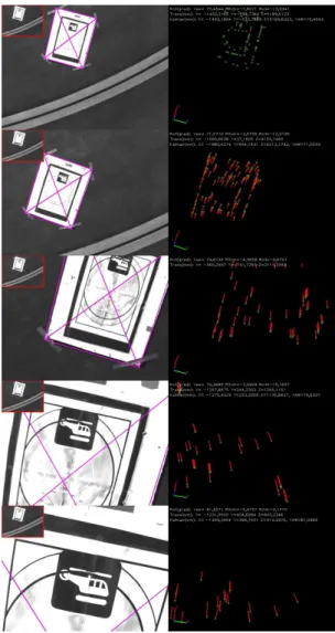
Figure 10 shows a landing sequence in which the 3D pose estimation based on a reference helipad is constantly estimated. The landing test begins when the UAV is hovering with an altitude of 5.2m, the figure shows the approach sequence when the helicopter is descending on the helipad. This figure also shows the original reference image, the current frame, the optical flow between last and current frame, the helipad coordinates in the current frame camera coordinate system and the Tait-Bryan angles obtained from the rotation matrix. Figure 11 shows the reconstruction of the flight test 1, using the IMU data.
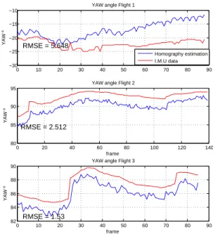
The 3D pose estimated using the visual system is com-pared with helicopter position estimated by the controller, with reference to the takeoff point (Center of the Helipad). Because the local tangent plane to the helicopter is defined in such a way that the X axis is the North position, theY axis is the East position and Z axis is the Down Position (negative), the measured X and Y values must be rotated according with the helicopter heading or Yaw angle, in order to be comparable with the estimated values obtained from the homographies. Figure 12 shows the estimated distance from the landmark with respect to the UAV during the descending approach and figure 13, shows the estimatedyaw angle.
Results show a good performance of the visual estimated values compared with the IMU data. In general, estimated and IMU data have the same behavior for test sequences. The estimated altitude position Z have a error for flight 1
Fig. 10. 3D pose estimation based on a helipad tracking using Robust
Homography estimation during a UAV landing process. Landing flight test
beginning at an altitude of5.2m. For all images, the reference imageI0 is
on the small rectangle on the upper left corner. Left it the current frame and Right the Optical Flow between the actual and last frame. Superimposed are the projection of the original rectangle, the translation vector and the Tait-Bryan angles.
with a RMSE of 0.32m, 0.23m in test 2 and 0.13m in test 3, showing a good performance of the estimator during the landing phase. Finally, the yaw angle is correctly estimated, presenting a maximum error of 5.6o between the IMU and the estimated data.
Results also have shown that the system correctly estimates the 3D position when a maximum of the 70 % of the landmark is out of the field of view of the camera (zoom). On Colibri project web pages [5] and [3] are available some videos showing these tests and the performance of the proposed system.
VI. CONCLUSIONS
−500 0
500
−200 0 200 400 600 800 1000 500 1000 1500 2000 2500 3000 3500 4000 4500 5000
U.A.V. East Position Local Plane (mm) U.A.V. North Position Local Plane (mm)
U.A.V. Up Position Local Plane (mm)
U.A.V. trajectory U.A.V. Heading
Fig. 11. 3D flight and heading reconstruction for the flight sequence show
on figure 10 (flight test 1)
0 10 20 30 40 50 60 70 80 90 0
2000 4000 6000
Z displacement Flight 1
Z mm
RMSE = 325.7
Homography estimation I.M.U data E.K.F
0 20 40 60 80 100 120 140
0 1000 2000 3000
Z displacement Flight 2
frame
Z mm RMSE = 237.1
0 10 20 30 40 50 60 70 80 90 1500
2000 2500 3000
Z displacement Flight 3
frame
Z mm
RMSE = 138.1
Fig. 12. Comparison between theZ axis displacement for homography
estimation and IMU data.
a Fuzzy controller in order to generate the commands for control the altitude of the unmanned helicopter to land on the helipad. The presented results shown a descend from a long distance, more than 5 meters, to the floor, obtaining the visual information even just the 30% of the helipad is in the camera field of view as is show in the last frame of the sequence. The optimal visual information allows to carry out the landing task in scenarios where the GPS dropouts make this task impossible to be accomplished. Furthermore, the obtained altitude information is more precise than the GPS-IMU onboard system, as are shown in real tests.
0 10 20 30 40 50 60 70 80 90 −30
−25 −20 −15 −10
YAW angle Flight 1
YAW º RMSE = 5.648
Homography estimation I.M.U data
0 20 40 60 80 100 120 140
80 85 90 95
YAW angle Flight 2
frame
YAW º
RMSE = 2.512
0 10 20 30 40 50 60 70 80 90 82
84 86 88 90
YAW angle Flight 3
frame
YAW º
RMSE = 1.53
Fig. 13. Comparison between theYawangle measured using homography
estimation and IMU data.
Future work includes to implement other Fuzzy controllers for the other possible movements of the UAV (Forward, Side and heading), in order to perform a total autonomous landing task in all axis. Use the implemented learning algorithm of the MOFS to improve the base of rules by the adaptation to manual flight. In addition, we are currently testing improved versions of the Lucas-Kanade optical flow, like the Inverse compositional algorithm (ICA) as well as evaluating the use of a different Kalman Filters for improved the 3D pose estimation.
ACKNOWLEDGMENT
The work reported in this paper is the consecution of several research stages at the Computer Vision Group -Universidad Polit´ecnica de Madrid. The authors would like to thank Jorge Le´on for supporting the flight trials, the I.A. Institute - CSIC for collaborating in the flights consecution, the Universidad Polit´ecnica de Madrid, the Consejer´ıa de Educaci´on de la Comunidad de Madrid and the Fondo Social Europeo (FSE) for some of the Authors’s PhD Scholarships. This work has been sponsored by the Spanish Science and Technology Ministry under the grant CICYT DPI 2007-66156.
REFERENCES
[1] Campoy, P., Correa, J.F., Mondrag´on, I., Mart´ınez, C., Olivares, M., Mej´ıas, L., Artieda, J.: Computer vision onboard UAVs for civilian
tasks. Journal of Intelligent and Robotic Systems.54(1-3), 105–135
(2009). DOI http://dx.doi.org/10.1007/s10846-008-9256-z
[2] Carnie, R., Walker, R., Corke, P.: Image processing algorithms for UAV ”sense and avoid”. In: Robotics and Automation, 2006. ICRA 2006. Proceedings 2006 IEEE International Conference on, pp. 2848– 2853 (2006). DOI 10.1109/ROBOT.2006.1642133
[4] Chaumette, F., Hutchinson, S.: Visual servo control. i.
ba-sic approaches. Robotics & Automation Magazine, IEEE
13(4), 82–90 (2006). DOI 10.1109/MRA.2006.250573. URL
http://dx.doi.org/10.1109/MRA.2006.250573
[5] COLIBRI: Universidad Polit´ecnica de Madrid. Computer Vision Group. COLIBRI Project. http://www.disam.upm.es/colibri (2009) [6] Criminisi, A., Reid, I.D., Zisserman, A.: A plane measuring device.
Image Vision Comput.17(8), 625–634 (1999)
[7] De Wagter, C., Mulder, J.: Towards vision-based uav situation
aware-ness. AIAA Guidance, Navigation, and Control Conference and
Exhibit (2005)
[8] Dong, T., Liao, X., Zhang, R., Sun, Z., Song, Y.: Path tracking and obstacles avoidance of uavs - fuzzy logic approach. In: Fuzzy Systems, 2005. FUZZ ’05. The 14th IEEE International Conference on, pp. 43– 48 (2005). DOI 10.1109/FUZZY.2005.1452366
[9] Fischer, M.A., Bolles, R.C.: Random sample concensus: a paradigm for model fitting with applications to image analysis and automated
cartography. Communications of the ACM24(6), 381–395 (1981)
[10] He, Z., V, L.R., R, C.P.: Vision-based UAV flight control and obstacle avoidance. In: Proceedings of the American Control Conference, p. 5pp (2006)
[11] Hutchinson, S., Hager, G.D., Corke, P.: A tutorial on visual servo control. In: IEEE Transaction on Robotics and Automation, vol. 12(5), pp. 651–670 (1996)
[12] Bouguet Jean Yves: Pyramidal implementation of the lucas-kanade feature tracker. Tech. rep., Intel Corporation. Microprocessor Research Labs, Santa Clara, CA 95052 (1999)
[13] Mejias, L., Saripalli, S., Campoy, P., Sukhatme, G.: Visual servoing approach for tracking features in urban areas using an autonomous
helicopter. In: Proceedings of IEEE International Conference on
Robotics and Automation, pp. 2503–2508. Orlando, Florida (2006) [14] Mondrag´on, I.F., Campoy, P., Martinez, C., Olivares-Mendez, M.A.:
3d pose estimation based on planar object tracking for UAVs control. In: Proceedings of IEEE International Conference on Robotics and Automation 2010 ICRA2010. Anchorage, AK, USA (2010) [15] Mondrag´on, I.F., Olivares-Mendez, M.A., Campoy, P., Martinez, C.:
Unmanned aerial vehicles uavs attitude, height, motion estimation and
control using visual systems. Autonomous RobotsIn Press, Corrected
Proof, – (2010). DOI DOI: 10.1007/s10514-010-9183-2
[16] Olivares, M., Campoy, P., Correa, J., Martinez, C., Mondragon, I.: Fuzzy control system navigation using priority areas. In: Proceedings of the 8th International FLINS Conference, pp. 987–996. Madrid,Spain (2008)
[17] Olivares, M., Madrigal, J.: Fuzzy logic user adaptive navigation control system for mobile robots in unknown environments. Intelligent Signal Processing, 2007. WISP 2007. IEEE International Symposium on pp. 1–6 (2007). DOI 10.1109/WISP.2007.4447633
[18] Olivares-Mendez, M.A., Campoy, P., Martinez, C., Mondragon, I.: Visual servoing using fuzzy controllers on an unmanned aerial vehicle. Eurofuse workshop 09, Preference modelling and decision analysis (2009)
[19] Saripalli, S., Sukhatme, G.S.: Landing a helicopter on a moving target. In: Proceedings of IEEE International Conference on Robotics and Automation, pp. 2030–2035. Rome, Italy (2007)
[20] Shengyi, Y., Kunqin, L., Jiao, S.: Design and simulation of the longitudinal autopilot of uav based on self-adaptive fuzzy pid
con-trol. In: Computational Intelligence and Security, 2009. CIS ’09.
International Conference on, vol. 1, pp. 634–638 (2009). DOI
10.1109/CIS.2009.253
[21] Shi, J., Tomasi, C.: Good features to track. In: 1994 IEEE Conference on Computer Vision and Pattern Recognition (CVPR’94), pp. 593–600 (1994)
[22] Siciliano, B., Khatib, O. (eds.): Springer Handbook of
Robotics. Springer, Berlin, Heidelberg (2008). DOI
http://dx.doi.org/10.1007/978-3-540-30301-5
[23] Simon, G., Berger, M.O.: Pose estimation for planar structures.
Com-puter Graphics and Applications, IEEE22(6), 46–53 (2002). DOI
10.1109/MCG.2002.1046628
[24] Simon, G., Fitzgibbon, A., Zisserman, A.: Markerless tracking using planar structures in the scene. In: Augmented Reality, 2000. (ISAR 2000). Proceedings. IEEE and ACM International Symposium on, pp. 120–128 (2000). DOI 10.1109/ISAR.2000.880935
[25] Smith, J., Nguyen, T.: Fuzzy logic based resource manager for a team of uavs. In: Fuzzy Information Processing Society, 2006. NAFIPS
2006. Annual meeting of the North American, pp. 463–470 (2006). DOI 10.1109/NAFIPS.2006.365454
[26] Sturm, P.: Algorithms for plane-based pose estimation (2000). URL http://perception.inrialpes.fr/Publications/2000/Stu00b
[27] Welch, G., Bishop, G.: An introduction to the kalman filter. Tech. rep., Chapel Hill, NC, USA (1995)
[28] Zhang, Z.: A flexible new technique for camera calibration. IEEE
Transactions on pattern analysis and machine intelligence 22(11),