Universidad EAFIT
Escuela de Ingenier´ıa
Grupo de Investigaci´
on de Mec´
anica Aplicada
MSc.Thesis
Wave propagation in a phase
transforming cellular material
Author
Sara Elena Rodr´ıguez G´
omez
[email protected]
Advisor:
Prof. Juan David G´
omez Cata˜
no
Co-Advisor:
Prof. Pablo Zavattieri
Abstract
The aim of this project is to explore the wave propagation properties in a phase transforming cellular material suitable for energy dissipation applica-tions. We pretend to understand how to control the dispersion behavior and switch the propagation properties when the phase transition is triggered. In the long-term, the main objective is to achieve a device with tunable band gaps and wave guide properties.
Contents
Introduction
5
State of the art
7
I
Wave propagation in periodic materials
9
1 Bloch analysis 10
1.1 Bloch-periodicity as boundary condition . . . 11
1.2 Fourier expansion of w(r) . . . 13
1.3 The reciprocal space . . . 14
1.4 The diffraction condition . . . 15
1.5 First Brillouin zone . . . 17
1.6 The band structure . . . 21
1.7 Dispersion relations for one dimensional lattice models . . . 25
2 Bloch-periodicity in the Finite Element Method 29 2.1 Implementation . . . 32
2.1.1 Code for Abaqus input files . . . 32
2.2 Construction of the band structure . . . 36
3 Classical problems in periodic materials 37 3.1 Elastic, homogeneous and isotropic infinite space . . . 37
3.2 Square inclusion . . . 42
II
Wave propagation in a bistable material
47
1 A cellular material that exhibits bistability 48
2 Building an open cell 51
3 Dispersion diagrams of the stable configurations 68
5 Modifying the topology 78
Introduction
Cellular materials offer a unique combination of properties making them highly ap-pealing and with a strong potential in different fields. They can exhibit high strength-to-weight and stiffness-strength-to-weight ratios; high compressive failure strains at nearly constant stress; low thermal conductivity combined with high mechanical strength at elevated temperatures; high surface area per unit volume together with high me-chanical strength and low density, among others [1–3]. With a controlled topology, relative density and geometry, novel materials are now possible thus widening its range of applications covering areas like medicine, package protection, chemical pro-cessing, waste management, aerospace and construction engineering.
Using the extended notion of solid state phase transformations to cellular solids, Restrepo et al. [4] designed a material that can switch its effective properties under a phase transformation. A phase transformation represents a change in the geome-try of the unit cell in such conditions that the topology remains unmodified, while experiencing changes in its effective properties. Thus, it is possible to generate pro-grammable devices with the advantages of cellular materials changing “on the fly”. On the other hand, the resulting phase transforming cellular material also offers good energy dissipation characteristics. This is achieved through an elastic bistable mechanism which produces a long stress-strain plateau, usually found in association to plastic behavior of materials.
A cellular material can also be regarded as a periodic material which inherently implies the existence of interesting phenomena associated to its wave propagation characteristics. First, periodic materials may exhibit stop bands introduced by Bragg scattering which produce frequency regions where waves are forbidden to propagate. Secondly, periodic materials may posses specific directions of preferred wave prop-agation or so-called directionality effects. The study of the effects known to exist in periodic materials in combination with the idea of bi-stable elemental cells with energy dissipation capabilities is a problem of interest on its own. In the particular case of Grupo de Investigaci´on en Mec´anica Aplicada of Universidad EAFIT, there is interest in exploring new alternatives to mitigate and attenuate elastic waves. In this project we conduct a preliminary study of phase transforming cellular materials aiming at identifying its potential in the frequency ranges of seismic waves.
conse-quence, it has directed its attention to the study of elastic wave propagation [5–8]. In the case of a phase transforming cellular material, we are interested in exploring the mechanisms that lead to wave control and energy dissipation (the last one al-ready covered in [4]). In general, with this work we seek to understand how a phase transformation changes the wave propagation properties of the cellular material and how to design appropriate unit cell geometries to achieve band gap tunability.
In the first part of the document we summarize the theoretical aspects of elastic wave propagation in periodic materials. In the first section of part I we present fun-damental concepts on Bloch analysis, while in the second we describe the basis of Bloch-periodicity conditions in the finite element method. The last section of part I is dedicated to two cases of elastic periodic materials studied with Bloch analysis (the homogeneous and isotropic material and the square inclusion).
State of the art
The study of periodic materials and structures can be traced back to Newton’s work on sound propagation in air and to Lord Rayleigh’s work in continuous periodic structures. Rayleigh showed that such materials can exhibit band gaps in the fre-quency spectrum, i.e., forbidden bands where waves can not propagate [10]. These and other early developments in the field are described in Brillouin’s book on peri-odic structures [11].
The fundamental analysis tool for the study of infinite periodic media can be identified in a theorem proved by G. Floquet [12] in 1880 and extended by F. Bloch in 1929 [13]. Bloch stated that in a crystal, the energy eigenstates for an electron can be written as a plane wave times a periodic function; this fact underlies the concept of electronic band structures and crystals properties1 which are well known
in solid-state physics. It turns out that a description in terms of Bloch waves applies to any wave-like phenomenon present in a periodic medium.
Periodic structures are differentiated as photonic crystals in electromagnetism and phononic crystals in acoustics and elasticity. The applications of phononic crys-tals are found, as expected, in wave control and filtering [14–19]. Also, there is important literature on the subjects of non-destructive testing [20], waveguiding and localization [21–25], signal sensing [26], wave demultiplexers passive devices [27–29], logic gates [30], liquid sensors [31], microfluidic manipulation [32], ultrahigh sensitiv-ity mass sensing above 100 GHz [33], sound collimation [34], refraction and focusing of sound waves [35,36], wave rectification and acoustic diodes [37,38], and “phoX-onic” crystals2 [39].
Another extension of phononic crystals applications, of particular interest to us, is active control or tunability. This branch focuses on the development of devices with the capability to change the location and size of band gaps “on the fly”, as well as the shapes of its band diagrams. For example, crystals where the orientation of the inclusions with respect to the incoming waves may be tuned during operation [40]; piezoelectricity to alter the cells [41–44]; light-induced substrate potential and elec-trorheological materials in which tuning is done via an external electric field [45,46];
1The classification of all crystals to metals, semiconductors and insulators is based on these
phenomena.
2Crystals that exhibit simultaneous phononic and photonic bandgaps coinciding at the same
magnetism to alter material elastic properties [47] and temperature control [48]. Also, there are some works related to the control of elastic waves like those using finite elastic pre-straining [49], mechanical instabilities to trigger large deformations [50] and nonlinear materials to tune band gaps [51–54].
To optimize the band gap characteristics, researches have identified two features in the design of phononic crystals: the unit cell topology [20,55–65] and the lattice symmetry [66]. The choice of the constitutive material phases and interweaving more than one lattice also provide possibilities for improving band gap characteristics [67].
Particularly in mechanics, before the introduction of phononic crystals theory as reported by Hussein [10], periodic structures had applications in composite ma-terials (modeled as periodic) [68,69], aircraft structures [70,71], multiblade tur-bines [72,73], impact resistant foam/cellular materials [74,75], periodic foundations for buildings [76,77], and multistory buildings and multispan bridges [78]. The field has been enriched notably with migration of concepts from phononic crystal treat-ment and recently, with the boom in metamaterials, broadly considered as examples of phononic materials except they have the added feature of exhibiting local reso-nance [9].
Starting in the 90s, we found contributions in elastic wave propagation for 2D spaces [79–83] and 3D phononic crystals [84–86]; sonic crystals, consisting of multiple phases of liquids and/or gases [14,80,87–89]; Rayleigh-type Bloch waves propagat-ing along free surfaces in 2D semi-infinite domains [90–93]; phononic crystals in the form of plates of finite thickness [26,94–103]; phononic crystals as MEMS [104,105]; other configurations as radial phononic crystals [106], quasicrystals [107] and frac-tals [108,109], and techniques to compute modes of evanescent Bloch waves [110,111].
Part I
Wave propagation in periodic
materials
A periodic material (PM) is defined as the repetition of a given motif in one, two or three space directions. The motif can be in the constituent material phases, the internal geometry, or the boundary conditions [10,112,113].
(a) Space Lattice (b) Motif (c) Material structure
Figure 1: To every lattice point, the motif is added till is formed the material struc-ture.
The description of a PM involves just the association of the motif to a lattice, which is a set of mathematical points (Figure1). The material is then formed by the addition of the motif to each point with the final result allowing the condition that: “in every point of the lattice the arrangement of the whole structure must look the same”. The lattice is thus said to be primitive and such condition implies that a PM is invariant under any translation of the form (for three dimensions 3):
T=n1a1+n2a2+n3a3, (1)
where ni ∈ Z and ai are basis vectors called primitive translation vectors
(withi= 1, 2, 3). They are formed by connecting the nearest neighboring points in the lattice and explicitly define the axes of periodicity. Figure2shows the primitive lattice in the description of a PM.
3For a perdiodicity in 2D, the translation is expressed with a
1 and a2. Similarly, in 1D the
a1 a2 a3
Primitive translation
vectors
Primitive cell
Lattice
Figure 2: Description of a periodic material in 3D.
The parallelepiped formed by the primitive axesa1,a2 anda3 contains the motif
and is called a primitive cell. This cell serves as building block of the material structure and will fill all the space by the repetition of suitable translation operations. Any local physical property of the PM is invariant under T, thus, the behavior of the whole material can be obtained just by studying the primitive cell.
1 Bloch analysis
The study of wave propagation in a PM can be conducted through Bloch-Floquet’s theorem which states that the wave function for a periodically repeated medium can be defined as:
u(r) =w(r)eik·r (2) where,ris the vector of spatial coordinates,kthe wavevector andw(r) is a func-tion with the same periodicity of the associated lattice, i.e.,w(r+T) = w(r).
The theorem was originally proved in the context of the Schr¨odinger equation with a periodic potential 4. According to [114]:
4The Schr¨odinger equation describes how the quantum state of a quantum system changes with
time, it predicts that wave functions can form standing waves, called stationary states: ˆHΨ(r) =
The eigenfunctions of the wave equation for a periodic potential are the product of a plane wave eik·r times a function w(r) with the periodicity of the crystal lattice. In general, equation (2) is a suitable solution for any wave equation where a physical property is represented as periodic, i. e.,
Lu(r) = ω2u(r) +f(ω),
where L is a differential operator and f(ω) a harmonic body force with angular frequencyω that is applied with the same periodicity of the lattice.
If we express equation (2) for a point in the space r+T, we will obtain
u(r+T) = w(r+T)eik·(r+T),
withT=niai being the translation vector. The functionw(r) has the periodicity
of the lattice, thus
u(r+T) =w(r)eik·(r+T). Replacing w(r) in equation (2) we have
u(r) =u(r+T)e−ik·(r+T)eik·r, which gives;
u(r+T) = u(r)eik·T. (3) Equation (3) is known as the Bloch-periodicity condition and is used as the boundary condition for a Boundary Value Problem (BVP) when studying PMs.
1.1 Bloch-periodicity as boundary condition
The elastodynamic wave equation in the frequency domain (reduced wave equation) reads [115]:
u=∇φ+∇ ×ψ, where ∇ ·ψ= 0 [115].
If we neglect body forces f, equation (4) is satisfied when:
∇2φ =−ω2
α2φ,
∇2ψ =−ω
2 β2ψ.
The fact that these expressions are also wave equations, implies that the dis-placement field is formed by two decoupled types of waves: a dilatational (gradient) term ∇φ corresponding to longitudinal waves or P-waves propagating with velocity α = λ+2ρµ1/2, and a distortional (rotational) term ∇ ×ψ corresponding to shear waves or S-waves propagating with velocity β =µρ1/2. Applying Bloch-Floquet’s theorem to the above (see equation (3)) gives:
φ(r+T) = φ(r)eik·T,
ψ(r+T) = ψ(r)eik·T, then,
u(r+T) =∇φ(r+T) +∇ ×ψ(r+T), =eik·T∇φ(r) +eik·T∇ψ(r), =eik·T[∇φ(r) +∇ψ(r)], =u(r)eik·T,
which shows that Bloch-Floquet’s theorem is also satisfied for the displacement field u.
(λ+µ)∇(∇ ·u) +µ∇2u=−ω2ρu in Ω, (5)
u(r+T) =u(r)eik·T in Γ, (6)
t(r+T) =−t(r)eik·T in Γ. (7) In the above t(r) is the surface traction vector.
1.2 Fourier expansion of
w
(r)
It has been stated that w(r) is a periodic function of r, with period a1, a2 and
a3 in the directions of the three material axes, respectively. It follows that the
condition w(r) = w(r+T) is better understood when expanded in Fourier series. Following [114] for a one-dimensional periodic function w(x) with period a in the direction of x, it is found that its sine and cosine Fourier expansion can be written like:
w(x) =w0+
X
p>0
[Cpcos (2πpx/a) +Spsin (2πpx/a)], (8)
where pare positive integers, and Cp, Sp are real constants.
It must be noticed that the factor 2π/a renders periodic the function w(x) with period a. Similarly, it shall be noticed that 2πp/a is a point in the reciprocal lat-ticeor Fourier space of the material 5. A term or point is allowed if it is consistent
with the periodicity of the material.
Equation (8) can be simplified into:
w(x) =X
p
wpei2πpx/a,
where the sum extends over all integers (p ∈ Z) andwp is a complex coefficient.
The extension to three dimensions of this last expression follows:
w(r) = X
G
wGeiG·r, (9)
where the set of vectors G leaves the equation invariant underT. These vectors are called the reciprocal lattice vectors.
1.3 The reciprocal space
The points in the reciprocal lattice can be defined by the set of vectors
G=m1b1+m2b2+m3b3,
wheremi ∈ Z and the basis vectorsbi are primitive vectors of the
recipro-cal lattice, withi= 1, 2, 3. A vectorGof this form is a reciprocal lattice vector and must keep the invariance of equation (9) under translationsT=n1a1+n2a2+n3a3:
w(r+T) = X
G
wGeiG·reiG·T =w(r) =⇒ eiG·T = 1.
To ensure the invariance, we construct the axis vectorsbiof the reciprocal lattice
using the expressions:
b1 = 2π
a2×a3
a1·a2×a3
, b2 = 2π
a3×a1
a1·a2 ×a3
, b3 = 2π
a1×a2
a1·a2×a3
. (10)
It shall be observed thata1,a2 anda3 are primitive vectors of the material lattice
(physical space) while b1, b2 and b3 are primitive vectors of the reciprocal lattice
(reciprocal space). They have the property
bi·aj = 2πδij with δij = 1 for i=j,
δij = 0 for i6=j.
From the above it is now evident that every material implicitly has two lattices: a material (direct) and a reciprocal lattice. Vectors in the direct lattice have dimen-sions of [length] while vectors in the reciprocal lattice have dimendimen-sions of [1/length], i.e., they have the units of wavelength and wavevector, respectively.
1.4 The diffraction condition
Consider the diffraction of an elastic wave of wavevector k by a volume element dV of a PM. The diffracted wave will have an outgoing wavevector k0 with a phase difference and amplitudeAd (see Figure3 ).
dV
k
k'
Δk
Figure 3: Diffraction of a plane wave by a volume elementdV in whichk+ ∆k=k0.
It can be assumed that the amplitude Ad is proportional to the local
proper-ties [114] (densityρ, Young’s ModulusE and Poisson’s ratioν). Since these proper-ties also have the periodicity of the lattice, the proportionality results in a periodic function having the form (see (9)):
w(r) = X
G
wGeiG·r.
The total amplitudeAdof the diffracted wave in the direction ofk0 is proportional
to the integral over the PM of w(r)dV times the phase factor ei(k−k0)·r. Then,
Ad=
Z
ei(k−k0)·rw(r)dV ≡ Z
e−i∆k·rw(r)dV,
where k−k0 =−∆k and ∆k measures the change in the wavevector when the wave is diffracted, i.e., a phase factor. Replacing for the Fourier components ofw(r) (Eq.(9)), the diffraction amplitude becomes:
Ad=
Z
e−i∆k·rX
G
wGeiG·rdV ≡ X
G Z
If the phase difference ∆kis equal to a particular reciprocal vector G, i. e.,
∆k=G, (11)
the argument of the exponential vanishes and the integral is equal toV wG. Also,
if ∆kdiffers significantly fromG,Ad is negligibly small which means that diffraction
is highly influenced by the periodicity of the material and it is interesting to identify which vectors satisfy this requirement. To this aim, it is convenient to write the expression given in (11) like:
k+G=k0, (k+G)2 =k02.
On the other hand, since we are considering elastic scattering, the energy of the incident wave is the same as that in the outgoing wave, in other terms: the angular frequencies must be the same ω = ω0. From relation ω = c|k|, where c is a wave velocity, it follows that|k|=|k0|. Substituting the above in the last expression gives the well knowndiffraction condition:
2k·G+G2 = 0. (12)
Since bothGand−Gare reciprocal lattice vectors, the result can also be written like:
2k·G=G2,
where one of the vectors satisfying the condition is recognized to be:
k=±1
2G.
This phenomenon is maximized when ∆k = G, where the diffracted beams are the result of a constructive interference6. From the superposition of two plane sine
waves with the same wavelength, it is clear that:
u(r) =A1sin (k·r) +A2sin (k·r+ϕ), = [A1 +A2] cos (ϕ/2) sin (k·r+ϕ/2),
6Diffraction phenomenon is described as the interference of waves according to the
which gives a wave whose amplitude depends on the phase ϕ. When the two waves are in phase (ϕ = 0), they interfere constructively; when the waves have opposite phase (ϕ=π), they interfere destructively. For an incident wave vector of the formk=±1/2G, the periodicity always causes a constructively interference, i.e, waves add in phase and yield the maximum amplitude for Ad.
1.5 First Brillouin zone
A Brillouin zone is said to be a vivid geometrical interpretation of the diffraction condition 2k·G =G2 [114] and it can be constructed as follows. Divide both sides by 4 gives 7
k· 1
2G=
1 2G
2
. (13)
and select a vectorGfrom the origin to a reciprocal lattice point. Then construct a plane normal to the vectorGat its midpoint. The resulting plane forms a part of a boundary zone as shown in Figure4. The wave vectors khaving the magnitude and direction required by (13) will be diffracted. It may be observed that this Brillouin construction encloses all such vectors, i.e., they go from the origin to any point along the constructed plane.
B
A
k1
k2
1/2 GB
O 1/2 GA
plane 1 plane 2
(a) Construction of Brillouin zones: The reciprocal lattice vector
GA connects the points OA; GB
connects OB. Planes 1 and 2 are the perpendicular bisectors of GA and
GB, respectively. Any vector from
the origin to the plane 1, such as k1,
will satisfy the diffraction condition
k1 · 1/2GA = (1/2GA)2; any vector
from the origin to the plane 2, such as
k2, will satisfy the diffraction condition
k2·1/2GB = (1/2GB) 2
.
(b) Some Brillouin zones: We have the square reciprocal lattice with lattice vectors in black lines; the bisectors planes are shown in colors. The central blue square is the smallest volume about the origin and is formed by the bi-sectors planes of the vectors G
connecting the nearest neighbor-ing points, it is called the first Brillouin zone.
Figure 4: Definition and construction of the first Brillouin zone.
From (11)8 it is known that k+ ∆k = k0 and ∆k = −G which means that
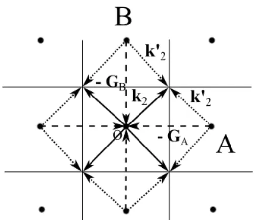
diffracted beams will be in the direction of k−G. In Figure 5 it is shown that a special geometric condition for all the diffracted beams corresponds to an incident wave generating a diffracted wave with direction k−G. Similarly, this last wave generates another diffracted wave and so on (all of them with the same magnitude).
A wave vectorkdrawn from the originO to any corner will satisfy the diffraction condition for bothGA and GB, thus, this wave generates two diffracted waves with
opposite directions that will act as new incident waves. As a result, the wave that points to a corner generates diffracted waves that point to the opposite corners. Such a feature will lead to a key concept in periodic materials as is the existence of band
gaps due to the formation of standing waves.
A
k1O - GA
k1 - GA = k'1
B
k'1
(a) Diffraction of a wave vectork1. The
diffracted wave will be in the direction ofk1−GAlike a mirror image, this last
wave act as a new incident wave and generate another one in the direction of k1. This process continues infinite
times.
A
k2
O - GA
k'2 k'2
B
- GB
(b) Diffraction of a wave vectork2that
points to a corner of the first Brillouin zone. This wave generate diffracted waves that point in the direction of the rest of the corners, i.e., waves travelling in opposite directions.
Figure 5: Direction of diffracted waves for the first Brillouin zone.
The set of planes that are perpendicular bisectors of the reciprocal lattice vectors divide the Fourier space into fragments, as shown in Figure 4. The central square is a primitive cell of the reciprocal lattice, called thefirst Brillouin zone and it is the smallest volume entirely enclosed by the bisectors planes.
It must be recalled that the reciprocal lattice space contains the information of the material periodicity: the set of vectors Grender invariant any periodic function under translationsT. Considering again Bloch-Floquet’s theorem from equation (2), and increasing the wave vectorkby a factorptimesG, i.e.,k+pGwithpan integer, gives:
u(r) = X
G
wGeiG·(r+T)ei(k+pG)·r,
=X
G
wGeiG·reiG·Teik·reipG·r,
=X
G
wGeipG·reiG·Teik·r,
=X
G
wGeipG·(r+T)eik·r,
where the property bi·aj = 2πδij (with i, j = 1,2,3) in the term eipG·T, yields:
eipG·T =e[ip(m1b1+m2b2+m3b3)·(n1a1+n2a2+n3a3)], =e[i2πp(m1n1+m2n2+m3n3)],
= 1.
The argument of the exponential contains the term 2π times an integerpbecause m1n1+m2n2+m3n3 is also an integer. Thus, increasing the wave vector by a factor ofpG means a translation of 2πp in the reciprocal lattice space and then, the initial expression u(r) remains invariant. It can be said that the information in k+pGis redundant, therefore, it is only neccesary to consider the values ofk in the interval of [0,2π] in all directions. The region enclosed by the interval will be defined around one node of the reciprocal lattice space where the origin is defined, this means that the first Brillouin zone fills the whole region of analysis: all the wave vectors k are considered in this zone. The primitive cell contains the information of the whole lattice and the other Brillouin zones have redundant information.
GA
Γ Χ
Μ
Figure 6: The irreducible Brillouin zone for a square lattice. The triangle Γ−X−M can describe completely the first Brillouin zone using symmetry operations.
1.6 The band structure
In a dispersive material (i.e., when the wave propagation velocity depends upon frequency) the dispersion relation ω = c|k| is no longer linear. This requires the distinction between two quantities: phase velocity and group velocity. The phase velocity cp is the velocity at which the phase of the wave (of any frequency
component) propagates in the space. It is defined as
cp =
ω
|k|k.ˆ (14)
The group velocity, on the other hand, is the velocity of propagation of the envelope of a wave package. It is defined by the relation:
cg =∇kω, (15)
where ∇k is the gradient of the angular frequency ω when written as a function
of the wave vectork, and ˆkis the unit vector in direction ofk. The group velocity is often thought of as the velocity at which wave energy or information is transported. In most cases this is accurate, however, if the wave is travelling through a dissipative medium, the group velocity ceases to have a clear physical meaning, [117]. Figure 7
Group velocity Phase velocity Non-dispersive
velocity
Wave number (k)
Angular f
reque
ncy (
ω)
Figure 7: Dispersion relation for a dispersive medium. The black solid line represent the dispersion curve, the phase velocity is the slope of the secant cutting the curve and the group velocity is the slope of the tangent in that cutting point.
The dispersion relation is also known as the band structureof a material as it describes the behavior of waves in terms of frequency bands. Among the methods to determine the band structure of complex systems one can identify wave expansions, finite difference time domain methods, finite element methods, multiple scattering theory, Rayleigh multipole and Green’s function methods (see [118]). Most of them cast the problem in the form of a generalized eigenvalue problem of the form:
K(k)−ω2Mu= 0, (16)
and where K and M are matrices containing information about the geometry and material parameters and u is the vector of degrees of freedom in the system. The band structure is found after finding the eigenfrequencies associated to the wave vectorsk along the borders of an irreducible Brillouin zone. .
As discussed earlier, the diffraction condition9 affects the dispersion relation of
a PM causing the formation of standing waves and the appearance of band gaps. Moreover, at Bragg’s diffraction wavelike solutions do not exist [114].
9Usually called Bragg’s diffraction and considered to be a special feature of wave propagation
The diffraction condition, (k+G)2 =k2, for a wave vector kin one-dimensional space becomes:
k=±1
2G=±q π a,
where G = 2πq/a is a reciprocal lattice vector and q is an integer. The first diffraction (and the first energy gap) occurs at k =±π/a, which in the wave vector space belongs to the region between [−π/a, π/a] and thus, to the first Brillouin zone of the 1D lattice. Other energy gaps occur for other values of the integer q.
As discussed previously, an incident wave vectork satisfying the diffraction con-dition will trigger the diffraction of waves traveling in opposite directions. In the current case of a 1D-space, the wave functions atk =±qπ/aare not traveling waves of the form eikx ore−ikx, but at these special values of k the waves are composed of equal parts traveling to the right and left thus forming a standing wave.
The Bragg diffraction condition is satisfied by the wave vectork =±qπ/a, there-fore, in the 1D case a wave traveling to the right is Bragg-diffracted to travel to the left, and vice versa. Each subsequent Bragg diffraction will reverse the direction of the wave. A wave that travels neither to the right nor to the left is a standing non-propagating wave as explained next. From the two traveling waves:
e±iπx/a = cosπx a
±isinπx
a
,
two different standing waves are formed and given by:
u(+) =eiπx/a+e−iπx/a = 2 cosπx a
,
u(−) =eiπx/a −e−iπx/a = 2isinπx a
.
Both standing waves are composed of equal parts of right and left directed trav-eling waves.
The energy of a system defined by equation (16), depends upon ω since the contributions to the potential and kinetic energy depend uponω:
E =EP +EK,
= 1
2K(ω)u
2(x) + 1 2ω
where ω(k) indicates that the frequency is a function of k.
A band gap in the band structure corresponds to an energy gap and there is an energy gap when a wave vectorksatisfies the diffraction condition therefore, leading to the appearance of standing waves. The energy of the system when k = ±π/a is given by:
E =EP =
1
2K(ω)u 2.
and it is evident that it only depends upon the potential energy due to the non-propagating nature of the standing waves.
cos²(πx/a) sin²(πx/a)
u²(x)
Figure 8: Distribution ofu2(x) in space. u(+)∝cos2(πx/a) andu(−)∝sin2(πx/a).
Figure8shows the space distribution ofu2(x). The energy of the system would be proportional to the envelope of this graph ifK(ω) were a constant. However, there is an energy difference between the standing waves sinceK(ω) is also distributed in the space. That is, it contains the information of the material properties and then, the information of the material periodicity. The energy difference between the standing waves creates an energy gap Eg [114] given by:
Eg =
1
2K(ω) [u(+)−u(−)].
The wave functions at the boundary of the Brillouin zone k = π/a, normalized over unit length of line, are √2 cos (πx/a) and √2 sin (πx/a). Assuming that K(ω) is a periodic function of the form
leads to an energy difference between the two standing wave given by:
Eg =
Z 1
0 1
2Kcos (2πx/a)
u2(+)−u2(−)dx,
= 2
Z 1
0 1
2Kcos (2πx/a)
cos2(πx/a)−sin2(πx/a)dx,
which after some manipulation10 becomes:
Eg = 2
Z 1
0 1
2Kcos (2πx/a)
cos2(πx/a)−sin2(πx/a)dx= 1 2K.
It can be observed that the energy gap is equal to the Fourier component of the material properties.
1.7 Dispersion relations for one dimensional lattice models
In elastodynamics, many complex structures can be represented by simple lattice models described in terms of systems of masses and springs. This section discusses the response of two of such systems, one corresponding to a simple mass and spring (Figure 9) and the other with two different masses (Figure11).
The period of the structure shown in Figure 9isa, while the lumped masses and spring stiffness aremandK respectively. The displacement at the arbitrary location xj is uj and the unit cell is repeated infinitely.
m m m
K K K
uj-1 uj uj+1
a Unit cell
Figure 9: Simple mass-spring lattice.
Now, consider the motion for the j-th mass governed by:
K(uj+1−uj)−K(uj−uj−1) = mu¨j.
If this motion is time harmonic with frequency ω, it follows that:
K(uj+1−uj)−K(uj −uj−1) +mω2uj = 0.
The Bloch-periodicity condition between consecutive masses reads:
uj−1 =uje−ika and uj+1 =ujeika,
therefore
Kuj 2−eika−e−ika
−mω2uj = 0.
On the other handeika+e−ika = 2 cos (ka) and 1−cos (ka) = 2 sin2(ka/2) which leads to:
4K m sin
2(ka/2)−ω2
uj = 0.
Since w > 0, it follows that for real values of k this equation has a nontrivial solution only if
ω(k) = 2
r
K
m|sin (ka/2)|=: 2ω0|sin (ka/2)|, (17) with ω0 =
q
K
m. This is the dispersion relation for the structure (see Figure 10).
It should be noticed that in the quasistatic limit k → 0, sin (ka/2) = ka/2 and ω(k) =kapK/m. The group velocity in this limit isdω/dk =apK/m.
0 0.5 1 1.5 2 2.5 3
-2 -1 0 1 2 3 4
ka/π
ω/ω
0
Figure 10: Dispersion curve for a simple mass-spring lattice. The shaded region corresponds to the first Brillouin zone. This eigenmode is called an acoustic mode because bothω and k go to zero simultaneously for some values.
In this simple one-degree-of-freedom system, there is only one eigenmode (called the acoustic mode) and therefore only one branch in the band diagram because there is only one direction of wave propagation. More eigenmodes and branches can be observed after increasing the complexity in the model.
For instance, consider now a two-mass-system (Figure11) with equations of mo-tion given by:
K(2Uj −uj −uj+1)−ω2M Uj = 0,
K(2uj −Uj−1−Uj)−ω2muj = 0.
M
K K K
uj
Uj
uj+1
a Unit cell
M
K Uj+1
K
uj-1
M
Uj-1
K
m m m m
Using the Bloch-periodicity condition
uj+1 =ujeika and Uj−1 =Uje−ika,
yields,
K2Uj−uj(1 +eika)
−ω2M Uj = 0,
K2uj −Uj(1 +e−ika)
−ω2muj = 0;
or using the matrix form ( ¯K−ω2M¯)¯u = ¯0 as
2K−ω2M −K(1 +eika)
−K(1 +e−ika) 2K −ω2m
Uj
uj
=
0 0
.
The resultant eigenvalue problem has a nontrivial solution if det( ¯K−ω2M¯) = 0 or equivalently if:
mM ω4−2K(m+M)ω2+ 4K2sin2(ka/2) = 0. It can be shown that positive eigenvalues correspond to:
ω(k) =
Km+M mM ±
K mM
p
m2+M2+ 2mMcos(ka)
1/2
,
0 0.5 1 1.5 2 2.5 3
-2 -1 0 1 2
ka/π
ω/ω
0
Band gap
Figure 12: Dispersion relation for a mass-spring lattice with two species of masses.
2 Bloch-periodicity in the Finite Element Method
The total potential energy functional of the system corresponding to equations (5 )-(7) is given by (see [113]):
Π(ω) =
Z
Ω
∗rs(r)Crskl(r)kl(r)dΩ−ω2
Z
Ω
ρ(r)u∗r(r)ur(r)dΩ−
Z
Γ
u∗r(r)tr(r)dΓ,
where the Einstein summation convention is implicit in the index notation and the complex conjugate is denoted by *. In the above expression the last term on the right corresponds to the work of the external traction and it implicitly contains the corresponding Bloch-periodicity conditions. After using standard finite element discretization ideas over the variational equation associated to Π, yields the following direct formulation:
K−ω2Mu=f.
In the above, the Bloch-periodicity conditions can be expressed through relations between the degrees of freedom (DOF) of opposite boundaries for the primitive cell of the PM.
u
iu
ltu
tu
rtu
ru
rbu
bu
lbu
l(a) Primitive Cell
Relevant nodes
u
iul
ulb
u
b(b) Reduced Cell: Rele-vant DOF in the primitive cell.
Figure 13: Primitive cell of finite elements. In the perimeter nodes, the subindex b denotes bottom,t=top, r=right andl=left. The domain nodes not in the perimeter are denoted as i=internal.
In the discretized domain, all of the elements will lie completely within the primi-tive cell and all boundary nodes will lie on the perimeter of the primiprimi-tive cell. On the other hand, there is no energy associated with M or K belonging to a neighboring primitive cell. However, there are extra degrees of freedom inusince the nodal DOF at the top and right boundaries of the primitive cell belong to neighboring primitive cells. For plane waves, the Bloch-periodicity conditions translate into a reduction of these nodal DOF. In the particular case of the primitive cell shown in Figure13, the system of equations correspond to the vectors:
u= [ul ur ub ut ulb urb ult urt ui]T ,
f = [fl fr fb ft flb frb flt frt fi]T .
From Bloch-Floquet’s theorem it follows that:
ur =uleikxTx, ut=ubeikyTy,
urb=ulbeikxTx, ult=ulbeikyTy,
urt =ulbei(kxTx+kyTy),
where (kx, ky) are the wave vector components andTx andTy are the translation
direction x and y.
The above relations can be expressed in matrix form as
ul ur ub ut ulb urb ult urt ui
| {z } u =
Il 0 0 0
IleikxTx 0 0 0
0 Ib 0 0
0 IbeikyTy 0 0
0 0 Ilb 0
0 0 IlbeikxTx 0
0 0 IlbeikyTy 0
0 0 Ilbei(kxTx+kyTy) 0
0 0 0 Ii
| {z }
A ul ub ulb ui
| {z }
uR
,
where I are identity matrices with subindex l and b denoting the boundary. Similarly, considering the equilibrium conditions
fr+fleikxTx = 0, ft+fbeikyTy = 0,
frt+frbeikxTx +flteikyTy +flbei(kxTx+kyTy) = 0,
or using its matrix form:
0 0 0 fi
| {z }
fR =
Il Ile−ikxTx 0 0 0 0 0 0 0
0 0 Ib Ibe−ikyTy 0 0 0 0 0
0 0 0 0 Ilb Ilbe−ikxTx Ilbe−ikyTy Ilbe−i(kxTx+kyTy) 0
0 0 0 0 0 0 0 0 Ii
| {z }
AH fl fr fb ft flb frb flt frt fi
| {z } f
,
where AH is the Hermitian transpose of A.
AHKA
| {z }
KR
−ω2AHMA
| {z }
MR
uR =fR,
and after neglecting the body forces fR as the reduced system
KRuR =ω2MRuR.
2.1 Implementation
A finite element implementation of the Bloch-analysis formulation can be developed following [113] through:
• A modification of the connectivity and also of the shape functions of the finite element method.
• An assembly of the mass and stiffness matrices without the boundary conditions and then, using elementary row/column operations to impose the boundary conditions.
In this work we have used the multi-point constraints tool (MPCs) from the com-mercial finite element code Abaqus in order to impose Bloch-periodicity conditions
2.1.1 Code for Abaqus input files
The used computer code writes the input files for the implementation of Bloch-periodicity conditions in Abaqus . The conditions are imposed through the multi-point constraint equation that describes a linear constraint between individual DOF. The equation used by Abaqus is
A1uP1 +A2u
Q
2 +...+AkuSk = 0,
where the subindex k =integer, represents the component of the solution vector u; A is the amplitude and P the selected point or node, i.e, A1uP1 represents the amplitude times the solution for the component 1 of theP-node. The Abaqus com-mand line reads
*EQUATION
Node, Component, Amplitude, Node, Component, Amplitude, ...
A particular case could be given by
*EQUATION 3
3, 1, 1, 45, 1, −cos (kx), 128, 1, −sin (kx)
that belongs to the equation
u31−cos (kx)u145−sin (ky)u1281 = 0.
The implemented code works for 2D rectangular cells and uses a rectangular win-dow for the sampling of the wave vector space. This is a grid ofSx×Sy data points
in direction of the Cartesian coordinates x and y. The pseudo codes are described in1 and 211.
11It is important to state that the method requires to duplicate the mesh to consider the imaginary
part, in this sense, the phase shift in the Bloch conditions is assigned to the solution using Euler’s equation:
Algorithm 1: Creates Abaqus input files with Bloch-periodicity conditions through MPCs.
Input :
Mesh: Nodes, Elements, Material Sets # Eigenvalues
Element Type Material Properties
Wave vector space sampling Sx, Sy.
Output:
Sx×Sy input files with Bloch-BC through MPCs.
/* Rectangular window of the wave vector space */
1 kx ← linspace(−π, π, Sx); 2 ky ←linspace(−π, π,Sy); 3 [kx, ky]← Meshgrid(kx,ky);
/* Phase assignment for every k */
4 Ckx←cos (kx);Skx←sin (kx);
5 Cky ←cos (ky);Sky ←sin (ky);
6 Ckxky ←cos (kx+ky); Skxky←sin (kx+ky);
/* Identical mesh for the imaginary part */
7 RNodes←Nodes; 8 RElmts←Elmts;
9 [IN odes, IElmts] =CopyMesh(RNodes,RElmts); 10 Nodes ←[RN odes;IN odes];
11 Elemts←[RElmts;IElmts];
/* Bloch-periodicity conditions */
Algorithm 2:Function to impose Bloch-periodicity conditions through MPCs.
1 Bloch-BC(N odes, P hases);
/* Perimeter nodes in the real and imaginary meshes */
2 Rre; RIm; /* Right */
3 Lre; LIm; /* Left */
4 Tre; TIm; /* Top */
5 Bre; BIm; /* Bottom */
6 LTre; LTIm; /* LeftTop */
7 RTre; RTIm; /* RightTop */
8 LBre; LBIm; /* LeftBottom */
9 RBre; RBIm; /* RightBottom */
10 for i= 1 : Sx×Sy do
11 print(’∗EQUATION’);
/* The following procedure will also apply for bottom and top nodes with the respective phases */
12 for j = 1 : #Lef tN odes do
/* Real part */
13 print(’3’);
14 print(’Rre(j),1,1,Lre(j),1,-Ckx(i),Lim(j),1,-Skx(i)’); 15 print(’Rre(j),2,1,Lre(j),2,-Ckx(i),Lim(j),2,-Skx(i)’);
/* Imaginary part */
16 print(’3’);
17 print(’Rim(j),1,1,Lim(j),1,-Ckx(i),Lre(j),1,-Skx(i)’); 18 print(’Rim(j),2,1,Lim(j),2,-Ckx(i),Lre(j),2,-Skx(i)’);
19 end
/* Corner points: same procedure for LT and RB with the
respective phases */
/* Real part */
20 print(’3’);
21 print(’RTre(j),1,1,LBre(j),1,-Ckxky(i),LBim(j),1,-Skxky(i)’); 22 print(’RTre(j),2,1,LBre(j),2,-Ckxky(i),LBim(j),2,-Skxky(i)’);
/* Imaginary part */
23 print(’3’);
24 print(’RTim(j),1,1,LBim(j),1,-Ckxky(i),LBre(j),1,-Skxky(i)’); 25 print(’RTim(j),2,1,LBim(j),2,-Ckxky(i),LBre(j),2,-Skxky(i)’);
2.2 Construction of the band structure
The determination of the band structure of a PM, requires the solution of an eigen-value problem for every k-point in the wave vector space. The required number of eigenvalues is approximately fixed by the desired number of curves in the dispersion relation.
The band structure is constructed for the wave vector values along the borders of the IBZ. The complete dispersion relation depends upon the cell dimension, i.e., for a 2D cell the wave vector will have two components, kx and ky in Cartesian
co-ordinates, then, the complete dispersion relationω(kx, ky) will be formed by surfaces.
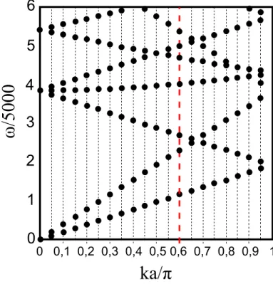
Figure 14 shows the construction of a band structure in a 1D problem, where there are twentyk-points between [0, π] and around seven eigenvalues for each value of k.
6
5
4
3
2
1
0
0 0,1 0,2 0,3 0,4 0,5 0,6 0,7 0,8 0,9 1
ka/π
ω/5000
3 Classical problems in periodic materials
This section, used for further reference, describes the results of previous analysis reported in the literature, see [112,113]. The section describes the following cases:
1. A homogeneous and isotropic material. 2. A square inclusion.
3.1 Elastic, homogeneous and isotropic infinite space
The material is infinite and uniform in the three space directions and is formulated in the xy plane after using a plane strain idealization. The primitive cell can be chosen arbitrarily since the material is homogeneous and isotropic (Figure 15). The elastic properties of the material (Aluminum) areE = 7.31×10¹⁰P afor the Young’s modulus,ν = 0.325 for the Poisson’s ratio, ρ= 2770kg/m3 for the mass density and the longitudinalα and transversal β velocities are α = 6198m/s and β = 3157m/s.
2d
a
2d
b
x y
Figure 15: Primitive cell: infinite isotropic and homogeneous elastic material.
For traveling plane waves, the wave vector norm or wave number is:
k =qk2
x+ky2.
Since there is no dispersion in a homogeneous and isotropic medium, the phase and group velocities coincide and the angular frequency is a linear function of the wave number
ω =ck=cqk2
x+ky2, (18)
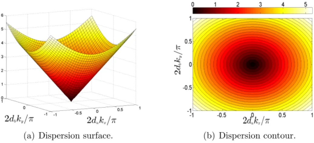
The dispersion relation in equation (18) represents the positive part of a cone in Cartesian coordinates, this cone must be obtained for every type of wave after solving the eigenvalue problem. Figure 16 shows the numerical results for this dispersion relation12.
(a) Dispersion surface. (b) Dispersion contour.
Figure 16: Numerical results for a homogeneous and isotropic material. These results correspond to the longitudinal wave (second calculated eigenvalue).
The dispersion relations are plotted in the First Brillouin zone, i.e., for a square cell 2dakx/π = [−1,1] and 2dbky/π = [−1,1]. Wave vectors k outside the First
Brillouin Zone can be written as:
kn,m =
kx+
nπ da
, ky+
mπ db
T
, (19)
wheren andm are integers counting cells to the right (or left) and up (or down). The vector [kx, ky]T belongs to the First Brillouin Zone.
The wave numbers can also be written as
kn,m =
s
kx+
nπ da
2
+
ky +
mπ db
2
,
and thus, the angular frequency would be
12In the literature, one frequently finds the iso-frequency contours: a projection of every formed
ωn,m =c
s
kx+
nπ da
2
+
ky +
mπ db
2
.
The complete band structure is constructed covering the range [0, π/2d] (2da =
2db = 2d): the IBZ since the material is isotropic. This region will capture also
the data corresponding to the wave vectors outside the Brillouin zone. Figure 17
represents the theoretical and numerical dispersion curves for the homogeneous and isotropic material.
ωn=0,m=0
P-wave S-wave
kx = nπ/da kx
ky
(a) Intersection of cones ω0,0(kx, ky)
with the planekx=nπ/da.
(b) Band structure. The solid lines are the theoretical solution, the dots are the numer-ical results.
Figure 17: Branches of the dispersion curves in a homogeneous and isotropic material.
For an incident wave taken in they-direction, withkx = 0, the branches of curves
that are observed correspond to
• Ifn =m = 0, the obtained curves are straight lines of the form ω=c|ky|.
• Ifn 6= 0 and m= 0, the curves are hyperboles, resulting from the intersection of the cones ω0,0(kx, ky) with the plane kx =nπ/d (Figure 17 a).
• If n 6= 0 and m 6= 0, the curves are folds of the hyperboles from the First Brillouin Zone.
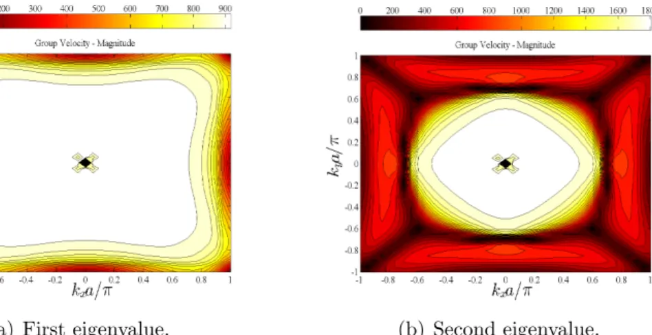
The group and phase velocities will provide an indication of the anisotropy of the material. The group velocity is calculated from the dispersion relation using equation (15). The result is a vector field whose components point in the direction of the greatest rate of increase of the function (perpendicular direction to each contour line in Figure 16), and with a magnitude given by the slope of the graph in that direction. Figure18 shows the group velocity vector field and its magnitude for the homogeneous and isotropic material.
(a) Vector field superimposed to the dis-persion contour. The arrows are perpen-dicular to each contour line.
(b) Magnitude: the colorbar value is nor-malized toα.
Figure 18: Group velocity for the second eigenvalue (longitudinal wave) of a homo-geneous and isotropic material.
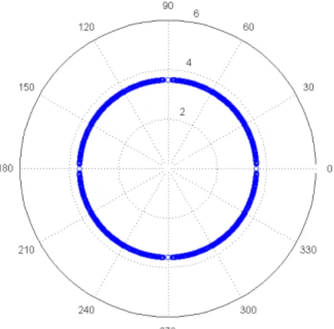
(a) Polar histogram: how many vector ar-rows point to a specific direction.
(b) Iso-frequency directivity: The direc-tion of group velocity for a specific value of the angular frequency (or contour level). The chosen value 2dω/5000≈3.8
Figure 19: Directivity of the material using the group velocity direction.
The polar histogram in Figure 19, shows that there is not a preferred direction of energy propagation in the material and there is the same number of wave vec-tors propagating energy in every direction. On the other hand, the iso-frequency directivity shows the preferred directions of energy propagation for just one value of the angular frequency, i.e., for a contour level in the dispersion contour. It is also observed how the chosen angular frequency does not present a preferred direction for energy propagation.
Figure 20: Phase velocity of the second eigenvalue (longitudinal wave)for a homoge-neous and isotropic material. The colorbar value is normalized to α.
3.2 Square inclusion
Consider now a cell composed of a square inclusion embedded in a matrix of an homogeneous material. The mechanical properties of the matrix are the same as in the previous case (Aluminum), while the inclusion has a Young’s modulus E = 9.2×10¹⁰P a, a Poisson’s ratioν = 0.33 and a mass density ρ= 8270kg/m3 (brass). The dimensions are presented in Figure21.
a
⅓
a
a
Figure 21: Primitive cell for a square inclusion.
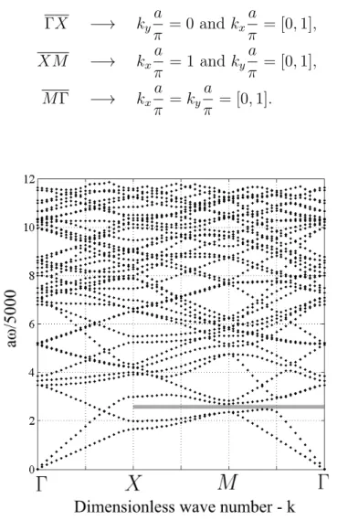
ΓX −→ ky
a
π = 0 and kx a
π = [0,1], (20) XM −→ kx
a
π = 1 andky a
π = [0,1], (21) MΓ −→ kx
a π =ky
a
π = [0,1]. (22)
Figure 22: Band structure for a square inclusion.
From Figure 22 it is evident that there are no full band gaps along the complete IBZ. This is in contrast with the diffraction condition which implies that band gaps appear every time kx,y = π/a. However, in the case of 2D elasticity, the fact that
can propagate along this region. In order to have a full band gap is thus necessary that the two forbidden regimes coincide.
6
3
1
0 1
Complete band gap
ka/π
aω/5000
Figure 23: Band structure for a bilayer cell.
From the analysis above it is clear that a complete band gap can be reached under very specific combinations of geometric conditions and material properties. These parameters control the slopes of the curves in the band structure. As a conclusion, in elasticity the existence of periodicity does not guarantee the existence of band gaps.
On the other hand, partial band gaps in the IBZ (usually known as pseudo band gaps) can exist. Considering again the square inclusion it is also observed that in the dark gray region there is a band gap for all the possible waves. However, it is constrained to the directions of X−M andM −Γ, i.e., for waves with an incidence of [0◦,45◦) and 45◦, respectively 13.
The dispersion contours of the first two eigenvalues for the square inclusion are shown in Figure24. At low frequencies both contours show the behavior of a homo-geneous and isotropic material, with stronger directional effects at higher frequencies. The directionality of the material is shown in Figure25.
13The segment ΓX represents the propagation in horizontal direction, i.e. 0◦;XM in the
(a) First eigenvalue. (b) Second eigenvalue.
Figure 24: Dispersion contour for a square inclusion.
0.5 1
1.5 2 2.5
30
210
60
240
90
270 120
300 150
330
180 0
(a) First eigenvalue.
0.5 1 1.5
2
30
210
60
240
90
270 120
300 150
330
180 0
(b) Second eigenvalue.
Figure 25: Polar histogram for a square inclusion. The data is normalized to the homogeneous and isotropic material, then, the red circle with radius= 1 corresponds to the homogeneous case.
The opposite behavior occurs for the second eigenvalue where it is observed that there is propagation along the diagonals but the preferred directions are around the principal axes, in the regions between (−30◦,30◦) and (−150◦,150◦) taken from each axis, approximately.
The iso-frequency directivity in Figure 26 supports what has been observed in the contours: the material behaves as homogeneous and isotropic at low frequencies, even at high frequencies for the second eigenvalue. The first eigenvalue presents pre-ferred directions of energy propagation at high frequencies: it is highly directional in the diagonals.
1000 2000 3000 4000 5000 30 210 60 240 90 270 120 300 150 330 180 0
(a) First eigenvalue.
1000 2000 3000 4000 5000 30 210 60 240 90 270 120 300 150 330 180 0
(b) Second eigenvalue.
Figure 26: Iso-frequency directivity for a square inclusion. Every color represents a value of the angular frequency.
(a) First eigenvalue. (b) Second eigenvalue.
Figure 27: Group velocity for a square inclusion.
(a) First eigenvalue. (b) Second eigenvalue.
Part II
Wave propagation in a bistable
material
This section is dedicated to the analysis of wave propagation in a phase transform-ing cellular material. The material was originally introduced by Restrepo et al. [4], in a project formulated between the Computational Multi-Scale Materials Modeling Laboratory of Purdue University, and the Research Laboratory in Smart Materials and Structures of General Motors Global Research & Development.
In the phase transforming cellular material, the primitive cell in its periodic rep-resentation has multiple stable configurations with each one of them corresponding to a phase. The change from one stable phase to the other is achieved trough large elastic deformations thus consuming energy during the process14. This feature com-bined with the periodic character of the material suggests the existence of complex and varying band structures opening the possibility for alternative forms of wave filtering and guiding. In this particular study the aim is to explore how to control the wave propagation behavior in the material and switch the propagation properties when the phase transition is triggered.
1 A cellular material that exhibits bistability
The cellular material consists of a primitive cell that can undergo phase transforma-tion. This corresponds to a change in geometry that leads to stable configurations while keeping its original topology.
The phase transforming cellular material (PXCM) is presented in Figure 29. The primitive cell comprises a compliant bistable mechanism that exhibits a force-displacement relation with a sawtooth shape (see Figure 30). The relation presents two limit points: (dI, FII) and (dII, FII), which define three regimes in the mechanical
response [4] described as follows:
• Regimes I and III are characterized by a positive stiffness, and represent the deformation of stable configurations of the primitive cell. These configurations correspond to a local minimum in the potential energy of the mechanism.
• Regime II is characterized by a negative stiffness and corresponds to a transition of the mechanism from one limit point to the other.
(a) Lattice. (b) Primitive cell.
Figure 29: The Phase Transforming Cellular Material (PXCM).
F
F
IU
F
IId
Id
IId
Regime I Regime II Regime III
.
Figure 30: Force Vs Displacement relation for the PXCM and its change of potential energy U [4].
The main question arising for the PXCM is whether the wave propagation is different for each stable phase, considering that there are only geometrical changes while the topology remains constant. This study explores how such particular fea-tures influence the dispersion relations of each phase and what are the controlling parameters in the wave propagation properties.
The three phases considered in this study are described by primitive cells referred to as open, intermediate and closed cell (see Figure 31). It is important to clarify that the study does no addresses the propagation properties during the phase change (Regime II). Furthermore, as the infinite material is deformed, the phase transition takes place one row at the time and the periodicity is broken. This suggests that the wave propagation properties also undergo a transition and the intermediate phase is an approximation when every row in the material has experienced half a collapse. In this study, we assume that during wave propagation the phase of the cellular material remains constant.
(a) Open cell (Regime I).
(b) Intermediate cell (Regime III for the upper half and Regime I for the lower half).
(c) Closed cell (Regime III).
.
Figure 31: Primitive rectangular cells used to describe the cellular material in each stable phase
In order to understand the response of each one of the considered phases, the analysis starts by studying the band structure of a progressively built open cell, that is a cell that is built in several stages after considering the contribution from addi-tional elements. This analysis is followed by the study of the three stable phases and by a final analysis considering pre-stresses. Accordingly, the last section explores the effects of a topological change in a closed cell.
I). Since the depth (cross section) of the PXCM is considered to be larger than any other delimited area inside the primitive cell, the model follows a plane strain idealization. Also, all of the primitive cells used for the analyses are rectangular and its IBZ correspond to the perimeter pointed in Figure 6 and equations (20)-(22). The mechanical properties and lattice parameters used during the analysis are:
• Young ModulusE = 1 GP a.
• Poisson’s ratio ν= 0.49.
• Density ρ= 1000kg/m3.
• For each phase a = 60 mm; in the open cell b ≈ 42 mm, intermediate cell b≈32mm and closed cell b ≈22 mm.
2 Building an open cell
In order to build the open cell, consider the five intermediate stages shown in Figure
32. Figure 33 displays the differences in dimensions between the different stages together with the proportions of the open cell compared to the first stage. The remaining cases will maintain the same dimensions as the components in the open cell. Figure34 shows the formed cellular materials based on each stage.
(a) Stage 1 (b) Stage 2 (c) Stage 3 (d) Stage 4
(e) Stage 5
.
(a) Open cell. (b) Stage 1.
.
Figure 33: Dimensions of the open cell and the stage 1.
Figure35shows the band structure for each one of the stages. The way in which the dots are connected is important as each line will correspond to a type of wave defining the limits of the band gap. However, the identification of the different types of waves for a connected line (i.e., telling if it is a P, S, or a combination mode) is still complex and an analysis of the eigenvectors would be necessary in order to have an idea of the propagation (of the deformation shape).
The most noticeable feature is the appearance of band gaps for the stage 1 and 3 and also, the fact that the eigenvalues decrease and the curves are compressed when new elements are considered in each following stage. With respect to the band gap of stage 1, it must be observed that although the cell is very similar to the stage 2, the band gap vanishes for the last one15.
Figure36 shows a close up of the band structure for the first nine eigenvalues of each stage. The existence of pseudo band gaps is evident, and also, it is observed how the band structure changes in stage 3 just because the addition of vertical bars.
15We can not say that stage 2 is the vertical alignment of two cells of stage 1, aligning two cells
results in a middle bar with thickness 1.484 mm, while that bar in stage 2 has a thickness of 2.5
(a)
Stage
1
(b)
Stage
2
(c)
Stage
3
(d)
Stage
4
(e)
Op
e
n
cell
.
Figure
34:
Cellular
materia
ls
based
on
th
e
primitiv
e
cells
considered
for
eac
h
(a)
Stage
1
(b)
Stage
2
(c)
Stage
3
(d)
Stage
4
(e)
Op
e
n
cell
.
Figure
35:
Band
structure
ev
olution:
stages
while
building
an
op
en
(a)
Stage
1
(b)
Stage
2
(c)
Stage
3
(d)
Stage
4
(e)
Op
e
n
cell
.
Figure
36:
Close
up
for
the
band
structure
of
eac
h
stage.
Nine
eigen
v
alues
are
In order to track the band gap found in stage 1, an analysis for cells correspond-ing to stage 2 with increascorrespond-ing density in the middle bar was conducted. We started fromρ= 1 kg/m3 with the assumption of absence of material. Figures 37show the band gap evolution.
The band structure of stage 1 and stage 2 with ρ = 1kg/m3 agree. More eigen-values appear as the density of the middle bar increases. By contrast the band gap, between ρ = 70 kg/m3 and ρ = 85 kg/m3 vanishes at a low value of the density considering the 1000 kg/m3 bound. The next step is exploring the region between 100 kg/m3 and 1000 kg/m3, where it was found that around 500 kg/m3 the band gap reappears but is lost again for higher values.
The anisotropy and directivity of each stage is now studied for the first two eigen-values. The dispersion contours in Figure 38and the polar histograms in Figure 39
and 40, show that all stages in both eigenvalues, except for the open cell, propagate energy preferably along the horizontal direction: the contours are compressed mainly towards they axis. The open cell presents a difference between the eigenvalues, the first one propagates energy mostly in the vertical direction while the second one does it in the horizontal direction.
We note also the similarity between stages 1 and 2. The contours are highly similar with the only difference in the polar histogram: stage 2 has a sharper angle around the horizontal direction. This could be explained from Figure 34, where the presence of an additional horizontal bar in the cell facilitates the energy propagation along this direction. From the cellular material of stages 3 and 4, it is observed that the lost in continuity of the vertical bar could also explain why the contours are com-pressed towards the y axis and the pronounced directionality along the horizontal direction.
Stage 1: First eigenvalue. Stage 1: Second eigenvalue.
Stage 2: First eigenvalue. Stage 2: Second eigenvalue.
Stage 3: First eigenvalue. Stage 3: Second eigenvalue.
Stage 4: First eigenvalue. Stage 4: Second eigenvalue.
Stage 5: First eigenvalue. Stage 5: Second eigenvalue.
In the case of the polar iso-frequency plot shown in Figure41, we obtain the direc-tivity behavior for a single angular frequency (each color corresponds to a frequency value). For stage 1 and 2, the first eigenvalue shows that at low frequencies the en-ergy is distributed along the horizontal and vertical directions. At higher frequencies the energy propagation tends to be in all directions. For the second eigenvalue, the first frequencies confine the energy around the horizontal direction of the material and the angle of energy propagation becomes wider as frequency increases.
Stages 3 and 4 are also similar. For both eigenvalues, the energy of lower fre-quencies is propagated in all directions, but as the frequency increases, the energy is distributed around the horizontal direction of the material. Stage 5 is different. The energy propagation at low frequencies is given in all directions for both eigenvalues. After increasing the frequency, the first eigenvalue presents energy propagation in the vertical direction and the second eigenvalue in the horizontal direction.
In Figures 42 and 44, we can identify what directions and magnitudes of the incident waves reach the highest values of the group and phase velocity. The axes in Figures 43and 45have different scales in order to appreciate the values variation.
Stage 1: First eigenvalue. Stage 1: Second eigenvalue.
Stage 2: First eigenvalue. Stage 2: Second eigenvalue.
Stage 3: First eigenvalue. Stage 3: Second eigenvalue.
Stage 4: First eigenvalue. Stage 4: Second eigenvalue.
Stage 5: First eigenvalue. Stage 5: Second eigenvalue.
Stage 1: First eigenvalue. Stage 1: Second eigenvalue.
Stage 2: First eigenvalue. Stage 2: Second eigenvalue.
Stage 3: First eigenvalue. Stage 3: Second eigenvalue.
Stage 4: First eigenvalue. Stage 4: Second eigenvalue.
Stage 5: First eigenvalue. Stage 5: Second eigenvalue.
Stage 1: First eigenvalue. Stage 1: Second eigenvalue.
Stage 2: First eigenvalue. Stage 2: Second eigenvalue.
Stage 3: First eigenvalue. Stage 3: Second eigenvalue.
Stage 4: First eigenvalue. Stage 4: Second eigenvalue.
Stage 5: First eigenvalue. Stage 5: Second eigenvalue.
Stage 1: First eigenvalue. Stage 1: Second eigenvalue.
Stage 2: First eigenvalue. Stage 2: Second eigenvalue.
Stage 3: First eigenvalue. Stage 3: Second eigenvalue.
Stage 4: First eigenvalue. Stage 4: Second eigenvalue.
Stage 5: First eigenvalue. Stage 5: Second eigenvalue.