Problem Understanding through Landscape Theory
Francisco Chicano
University of Málaga, Spainchicano@lcc.uma.es
Gabriel Luque
University of Málaga, Spaingabriel@lcc.uma.es
Enrique Alba
University of Málaga, Spaineat@lcc.uma.es
ABSTRACT
In order to understand the structure of a problem we need to measure some features of the problem. Some examples of measures suggested in the past are autocorrelation and fitness-distance correlation. Landscape theory, developed in the last years in the field of combinatorial optimization, pro-vides mathematical expressions to efficiently compute statis-tics on optimization problems. In this paper we discuss how can we use landscape theory in the context of problem un-derstanding and present two software tools that can be used to efficiently compute the mentioned measures.
Categories and Subject Descriptors
I.2.8 [Artificial Intelligence]: Problem Solving, Control Methods, and Search
General Terms
Theory, AlgorithmsKeywords
Fitness Landscapes, Elementary Landscapes, Problem Un-derstanding, Quadratic Assignment Problem, Unconstrained Quadratic Optimization
1.
INTRODUCTION
Landscape theory is a set of definitions and theorems that allows one to analyze optimization problems in connection with a neighborhood structure defined over the search space. We are interested in the applications of the theory to Com-binatorial Optimization. However, this theory has appli-cations in Chemistry [19], Biology [24] and Physics [12]. One of the main goals of the theory is to better understand the structure of the optimization problems. Thanks to this deeper understanding we are supposed to be able to define new search operators, search strategies or even determine the optimal values for the parameters of the algorithms used to solve a given problem.
Permission to make digital or hard copies of all or part of this work for personal or classroom use is granted without fee provided that copies are not made or distributed for profit or commercial advantage and that copies bear this notice and the full citation on the first page. To copy otherwise, to republish, to post on servers or to redistribute to lists, requires prior specific permission and/or a fee.
GECCO’13 Companion, July 6–10, 2013, Amsterdam, The Netherlands.
Copyright 2013 ACM 978-1-4503-1964-5/13/07 ...$15.00.
There is a special kind of landscapes, called elementary landscapes, with nice properties. In particular, they are characterized by Grover’s wave equation [14]:
avg{f(y)} y∈N(x)
=f(x) +k
d f¯−f(x)
, (1)
wheredis the neighborhood size, |N(x)|, which we assume the same for all the solutions in the search space, ¯f is the average value of the objective function in the whole search space and k is a constant. Either k or ¯f can usually be efficiently and accurately computed from the problem data or by a random sampling of the search space.
The advantage of an expression like (1) is that it allows one to compute a statistics (the average in the neighbor-hood) from the value of a function inx. We must highlight here that if (1) were not true, we would need to evaluate ev-ery solution inN(x) in order to compute the average in the neighborhood. Thus, landscape theory gives us results that allow us to compute in an efficient way some non trivial statistics related to the distribution of the objective func-tion. This property is present in most of the results of land-scape theory, as we will see along the next sections.
In this paper we will focus mainly on three measures that can be efficiently computed using landscape theory. They are the autocorrelation, the fitness-distance correlation and the expected fitness after bit-flip mutation. The first two statistics have been considered as measures for problem hardness. None of them is a perfect measure of the hardness of a problem and both have been criticized in the past. How-ever, they are used even in some recent works. In this paper we will see how they can be efficiently computed using land-scape theory under some conditions and we provide software tools to do it. Regarding the expected fitness after bit-flip mutation, it has some links to runtime analysis, which is a direct measure of problem hardness. But, more interesting is the fact that the elementary decomposition of a combi-natorial optimization problem has a one-to-one relationship with the expectation curves (depending on the probability of mutation) of bit-flip.
above can only be applied to concrete problems. During the last three years we have frequently implemented code snip-pets and algorithms to check empirically the results provided by the theory. We think the resulting software could be use-ful for researchers interested in problem understanding. For this reason, we present, as the main contribution of this pa-per, two of the implemented applications and provide links to them. In one case we provide a web application that ev-eryone can use without installing anything and in the other case we provide a GUI-based application.
The organization of the paper is as follows. In Section 2 we provide some background on landscape theory. Sections 3, 4 and 5 discusses how landscape theory can be used to effi-ciently compute the autocorrelation, fitness-distance corre-lation and expected fitness after bit-flip mutation in a com-binatorial optimization problem. Section 6 presents the soft-ware tools developed in the last years that implement the al-gorithms to efficiently compute the measures described and other parameters related to landscape theory. Finally, Sec-tion 7 concludes the work and describes future work.
2.
BACKGROUND
In this section we present some fundamental results of landscape theory. We will only give a soft introduction to general concepts of landscape theory. We refer the reader interested in a deeper exposition of this topic to the survey in [17].
A landscape for a combinatorial optimization problem is a triple (X, N, f), whereX is the solution set,f :X 7→R
defines the objective function and N is the neighborhood function, which maps any solutionx∈X to the setN(x) of points reachable fromx. Ify∈N(x) then we say thatyis a neighbor ofx.
The pair (X, N) is calledconfiguration space and can be represented using a graphG(X, E) in whichX is the set of vertices and a directed edge (x, y) exists inE ify ∈N(x) [5]. We can represent the neighborhood operator by its ad-jacency matrix
Ax,y=
1 ify∈N(x),
0 otherwise. (2)
Any discrete function,f, defined over the set of candidate solutions can be characterized as a vector in R|X|. Any |X| × |X| matrix can be interpreted as a linear map that acts on vectors inR|X|. For example, the adjacency matrix
Aacts on functionf as follows
Af=
P
y∈N(x1)f(y)
P
y∈N(x2)f(y)
.. . P
y∈N(x|X|)f(y)
. (3)
The componentxof this matrix-vector product can thus be written as:
(Af)(x) = X
y∈N(x)
f(y), (4)
which is the sum of the function value of all the neighbors of
x. When a neighborhood is regular the so-calledLaplacian matrix is defined as∆=A−dI. Stadler defines the class ofelementary landscapes where the functionf is an eigen-vector (or eigenfunction) of the Laplacian up to an additive constant [18]. Formally, we have the following:
Definition 1. Let (X, N, f) be a landscape and ∆ the Laplacian matrix of the configuration space. The landscape is said to be elementary if there exists a constantb, which we call offset, and an eigenvalueλof−∆such that(−∆)(f−
b) =λ(f−b).
We use eigenvalues of−∆ instead of∆ to have positive eigenvalues [5]. In connected neighborhoods (the ones we consider here) the offsetbis the average value of the function over the whole search space: b = ¯f [11]. In elementary landscapes, the average value ¯fcan be usually computed in a very efficient way using the problem data. That is, it is not required to do a complete enumeration over the search space.
Taking into account basic results of linear algebra, it is not difficult to prove that iff is elementary with eigenvalue
λ, af+b is also elementary with this same eigenvalue λ. Furthermore, in regular neighborhoods, ifgis an eigenfunc-tion of −∆ with eigenvalueλ theng is also an eigenvalue ofA, the adjacency matrix, with eigenvalued−λ. The av-erage value of the fitness function in the neighborhood of a solution can be computed using the expression:
avg{f(y)} y∈N(x)
= 1
d(Af)(x). (5)
Iffis an elementary function with eigenvalueλ, then the average is computed as:
avg{f(y)} y∈N(x)
= avg
y∈N(x){
f(y)−f¯}+ ¯f
=1
d(A(f−f¯))(x) + ¯f= d−λ
d (f(x)−f¯) + ¯f
=f(x) +λ
d( ¯f−f(x)), (6)
and we get Grover’s wave equation [14]. In the previous expression we used the fact thatf−f¯is an eigenfunction of
Awith eigenvalued−λ.
The wave equation makes it possible to compute the av-erage value of the fitness functionfevaluated over all of the neighbors ofxusing only the valuef(x), that is, it provides a way of computing non-trivial statistics with a low com-putational cost. The previous average can be interpreted as the expected value of the objective function when a ran-dom neighbor of xis selected using a uniform distribution. This is exactly the behaviour of the so-called1-bit-flip mu-tation [13]. It could seem that the restriction imposed by Grover’s wave equation cannot be frequently found in op-timization problems. However, there are some well-known NP-hard problems using common neighborhoods that are el-ementary landscapes. This is the case of the Not All Equals SAT problem, the Travelling Salesman Problem, the Graph Coloring problem, etc. The interested reader can find ex-amples of elementary landscapes in [25, 26].
Certainly, a landscape (X, N, f) is not always elementary, but even in this case it is possible to characterize the function
f as the sum of elementary landscapes, called elementary components of the landscape. When the neighborhoodN of the landscape is symmetric there exists an orthogonal basis of the space of functions composed of elementary landscapes. Let us denote this basis with θλ,iwhere λis the eigenvalue
different vectors with the same eigenvalue. Then a Fourier expansion offis
f=X
λ X
i
aλ,iθλ,i,
where the valuesaλ,i=hθλ,i, fiare the Fourier coefficients.
Using this Fourier expansion it is possible to compute the landscape decomposition by summing the terms with the same eigenvalue. Each elementary component can be com-puted as
fλ= X
i
aλ,iθλ,i. (7)
A special case is that off0, the elementary landscape with
λ = 0. If we assume that the neighborhood is connected then f0 is the constant value ¯f. Finding the elementary components of a given optimization problem is not a trivial task. In the last years we can find some works devoted to the task of finding this decomposition for some well-known problems. Along the paper we will cite the corresponding works when needed. The reader interested in finding such a decomposition for her/his favourite optimization problem can find a methodology to do it in [11].
3.
AUTOCORRELATION
Theautocorrelation coefficientξof a problem is a param-eter proposed by Angel and Zissimopoulos [1] that gives a measure of its ruggedness. The same authors showed later in an empirical study thatξ seems to be related with the performance of Simulated Annealing [2]. Another measure of ruggedness defined by Garc´ıa-Pelayo and Stadler is the
autocorrelation length [12], denoted withℓ. The autocorre-lation length is specially important in optimization because of the autocorrelation length conjecture, which claims that in many landscapes the number of local optimaM can be estimated by the expression [20]:
M ≈ |X| |X(x0, ℓ)|
, (8)
whereX(x0, ℓ) is the set of solutions reachable from x0 in
ℓor less local movements. The previous expression is not exact, but an approximation. It can be useful to compare the estimated number of local optima in two instances of the same problem. In effect, for a given problem in which (8) is valid, the higher the value ofℓthe lower the number of local optima. In a landscape with a low number of local optima, a local search strategy cana priorifind the global optimum using less steps.
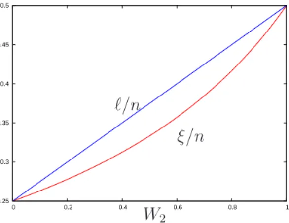
In many problems, ξ andℓare directly related. That is, when one of them increases the other does the same. As an example we consider the Unconstrained Quadratic Op-timization (UQO). We can observe in Figure 1 that both autocorrelation measures,ξ andℓ, increase withW2 (spec-tral coefficient, see below) and their values are betweenn/4 whenW2= 0 andn/2 whenW2= 1. However, the curve of
ℓis linear while the one ofξis non-linear.
In the context of the autocorrelation length conjecture, this could explain why Angel and Zissimopoulos observed a better performance of SA when the problem instances had a higher value forξ. Instances with higherξmost probably would have higherℓand this most probably would mean a lower number of local optima in the instance, so it is easier
0.25 0.3 0.35 0.4 0.45 0.5
0 0.2 0.4 0.6 0.8 1
ξ/n
ℓ/n
W2
Figure 1: Value of ξ/nandℓ/n againstW2.
for a local search algorithm like SA to solve the problem instance. A recent work based also in QAP supports this idea [9].
Let us discuss now how can we efficiently computeξ and
ℓif we know the elementary landscape decomposition of a problem. Let us consider a random walk {x0, x1, . . .} on the solution space such thatxi+1∈N(xi). The Weinberger
autocorrelation function ris defined as:
r(s) =avg{f(xt)f(xt+s)}x0,t−avg{f(xt)}
2
x0,t
avg{f(xt)2}x0,t−avg{f(xt)}
2
x0,t
, (9)
where the averages are computed over all the starting solu-tions x0 and all the solutions in the sequence [24]. Based on this function the autocorrelation coefficient and the au-tocorrelation length are defined as:
ξ= 1
1−r(1), (10)
ℓ= ∞ X s=0
r(s). (11)
Stadler [18] proved that iff=P
iaiφiis a Fourier
expan-sion of f in a landscape, then the autocorrelation function off is given by
r(s) =X
i6=0
a2i P
j6=0a2j
1−λdi s
, (12)
whereλiis the eigenvalue associated to the elementary
func-tionφi. As a consequence, the valuer(1) is:
r(1) = P
i6=0a 2
i
1−λi d P
j6=0a2j
= 1− P
i6=0a 2
i λi
d P
j6=0a2j
,
and the autocorrelation coefficient can be computed as
ξ= d P
j6=0a2j P
i6=0a2iλi
. (13)
The sum of the squared Fourier coefficientsa2
j associated
to the same eigenvalue λi is |X|(fi2−fi
2
), where fi is the
sum of all the elementary components aiφi with the same
eigenvalue λi and the overline represents the average over
coefficientsa2jwithj6= 0 is|X|(f2−f
2
). Introducing these two expressions in (13) we can write:
ξ= P
i6=0(fi2−fi
2 )λi
d(f2−f2) !−1
=
X i6=0
Wi
λi
d
−1
,
where the valuesWi are called spectral coefficients and are
defined as
Wi=
f2
i −fi
2
f2−f2. (14)
The autocorrelation length ℓcan also be expressed with the help of (12) as:
ℓ= ∞ X s=0
r(s) =dX
i6=0
Wi
λi
. (15)
Thus, the problem of computing the autocorrelation coef-ficient and length is reduced to the problem of finding the spectral coefficientsWi. These coefficients have been
com-puted for some NP-hard combinatorial optimization prob-lems. Chicano et al. [10] provide expressions for the au-tocorrelation measures in the case of QAP. They do not provide any algorithm to do it in the paper but they imple-mented anO(n2) algorithm to compute the autocorrelation measures which is available on-line(see Section 6). For il-lustration purposes we show here the values for autocorrela-tion measures and spectral coefficient of the Unconstrained Quadratic Optimization (UQO). The details can be found in [6]. The autocorrelation coefficient and length is given by the following expressions:
ξ= n
2(2−W2), (16)
ℓ= n(1 +W2)
4 , (17)
where n is the size of the problem (length of the binary solutions) andW2is given by:
W2=
f2 2
f2−f2. (18)
The expressions forf2
2,f2 andf 2
are:
f2= 1 16
n X i,j=1
qij+ n X i=1
qii !2
, (19)
f2 2 =
1 16
n X i=1
v2i, (20)
f2=
n X i,j=1
n X i′,j′=1
qijqi′j′
2|{i,j,i′,j′}|. (21)
The previous expressions can be computed at most in
O(n4). Sutton et al. [22] showed how the autocorrelation function r(s) can be computed for all the pseudo-Boolean functions using the one-flip neighborhood. The previous ex-pression is just a particular case of the Sutton’s exex-pression. In their work they provided expressions for the MAX-3-SAT problem.
4.
FITNESS-DISTANCE CORRELATION
The Fitness-Distance Correlation (FDC) is a measure in-troduced by Jones and Forrest [15] to measure problem dif-ficulty. Given all the solutions in the search space, it com-putes the correlation coefficient between the fitness values of these solutions and the Hamming distances of the solutions to their nearest global optimum. In the case of an optimiza-tion problem defined over a binary soluoptimiza-tion space we can define FDC as follows.Definition 2. Given a functionf :Bn7→
Rthe fitness-distance correlation forf is defined as
r= Covf d
σfσd
, (22)
where Covf d is the covariance of the fitness values and the
distances of the solutions to their nearest global optimum,σf
is the standard deviation of the fitness values in the search space andσdis the standard deviation of the distances to the
nearest global optimum in the search space. Formally:
Covf d=
1 2n
X x∈Bn
(f(x)−f)(d(x)−d),
f= 1 2n
X x∈Bn
f(x), σf = s
1 2n
X x∈Bn
(f(x)−f)2,
d= 1 2n
X x∈Bn
d(x), σd= s
1 2n
X x∈Bn
(d(x)−d)2, (23)
where the functiond(x)is the Hamming distance betweenx
and its nearest global optimum.
The FDCr is a value between −1 and 1. The lower the absolute value ofr, the more difficult the optimization prob-lem is supposed to be. The exact computation of the FDC using the previous definition requires the evaluation of the complete search space. It is required to determine the global optima to defined(x) and compute the statistics fordandf. If the objective functionf is a constant function, then the FDC is not well-defined, since σf = 0. The next theorem,
extracted from [8], provides an exact expression for FDC in the case in which there exists one only global optimum x∗
and we know the elementary landscape decomposition off.
Theorem 1. Let f be an objective function whose
ele-mentary landscape decomposition isf=Pn
p=0f2p, wheref0
is the constant functionf0(x) =f and eachf2p withp >0
is an order-pelementary function with zero offset. If there exists only one global optimum in the search space x∗, the FDC can be exactly computed as:
r= −f2(x ∗)
σf√n
. (24)
The result of the previous theorem starts an interesting discussion. In Section 3 we mentioned that some works on landscape analysis claim that the ruggedness of a landscape is related to its hardness [3]. In particular, the autocor-relation coefficientξ and the autocorrelation length ℓ of a problem are two measures proposed to characterize an ob-jective function in a way that allows one to estimate the performance of a local search method. Also a relationship has been noticed between the autocorrelation length and the expected number of local optima of a problem [12], in agreement with the autocorrelation length conjecture. In summary, empirical and theoretical results support the hy-pothesis that a rugged landscape is more difficult than a problem with a smooth landscape.
In the case of the elementary functions defined over binary strings, the functions with higher order are more rugged than the ones with lower order. The order-1 elementary landscapes are the smoothest landscapes and, in fact, they can always be solved in polynomial time. Following this chain of reasoning, in a general landscape, the elementary components with order p > 1 are the ones that make the problem difficult. However, from Theorem 1 we observe that only the order-1 elementary component of a function f is taken into account in the computation of the FDC. This fact poses some doubts on the value of the FDC as a measure of difficulty of a problem, since FDC is shown to neglect the rest of information captured in the higher order components. This is true under the assumption that one single global optimum exists in the search space. The doubts on FDC as being a difficulty indicator have also been raised by other authors. Two examples are the work by Tomassini et al. [23] focused on genetic programming and the one by Bierwirth et al. [4] based on the Job Shop Scheduling.
If the objective function is elementary, then the expression of the exact FDC is specially simple:
r= (
f−f(x∗)
σf√n ifp= 1,
0 ifp >1. (25)
The previous equation states that only elementary land-scapes with orderp= 1 have a nonzero FDC. Furthermore, the FDC does depend on the value of the objective function in the global optimumf(x∗) and the average valuef, but not on the solution x∗ itself. We can also observe that if we are maximizing, thenf(x∗) > f and the FDC is neg-ative, while if we are minimizingf(x∗) < f and the FDC is positive. The order-1 elementary landscapes can always be written as linear functions and they can be optimized in polynomial time. That is, iff is an order-1 elementary function then it can be written in the following way:
f(x) =
n X i=1
aixi+b. (26)
whereaiandbare real values. If such a linear function has
only one global optimum (that is,ai6= 0 for alli). The FDC
can be computed using the expression:
r= − Pn
i=1|ai| p
nPn i=1a2i
, (27)
which is always in the interval−1≤r < 0. When all the values ofai are the same, the FDC computed with (27) is −1. This happens in particular for the Onemax problem. But if there exist different values forai, then we can reach
any arbitrary value in [−1,0) forr. The next result provides a way to design a linear function with the value ofrwe want.
Theorem 2. Letρ be an arbitrary real value in the
in-terval [−1,0), then any linear function f(x) given by (26) wheren >1/ρ2,a2=a3=. . .=an= 1anda1 is
a1 =
(n−1) +n|ρ|p
(1−ρ2)(n−1)
nρ2−1 , (28)
has exactly FDCr=ρ.
Theorem 2, also extracted from [8] provides a solid argu-ment against the use of FDC as a measure of the difficulty of a problem. In effect, we can always build an optimization problem based on a linear function, which can be solved in polynomial time, with an FDC as near as desired to 0 (but not zero), that is, as “difficult” as desired according to the FDC. However, we have to highlight here that for a given FDC valueρwe need at leastn >1/ρ2 variables. Thus, an FDC nearer to 0 requires more variables.
Let us discuss now how can we use (24) in order to com-pute FDC for a given problem. Observe that we need the global optimum but most probably we don’t know that global optimum (that’s the reason we are interested in solving that problem). This is a drawback not only of our expression, but of any other procedure to compute FDC. In all the cases we need the global optima. Thus, we cannot compute the ex-act FDC in general, but an approximation. One empirical procedure to compute FDC would consist in sampling the search space, evaluating the fitness in all these solutions, computing the distances between any pair of solutions and, finally, computing FDC using (22). This procedure requires to store all the sampled points in memory until we decide which one is the optimum and we compute all the distances between them. In this case our expression (24) have some advantages to simplify the procedure. First, we don’t need to store all the points in memory, just the optimal one. Thus, the sampling can be just a trajectory-based strategy (guided or not) that tries to find the global optimum. Second, once we have a solutionx∗that will be used in the computation of FDC, we have just to evaluate f2 on it and apply (24) to getr. Third, the FDC value computed in this way takes into account not only the sampled points, but all the points in the search space, that is, it is a statistic that considers the entire search space. Thus, we would expect it to be more accurate than the empirical FDC computed using only the sampled values. We have, however, to clarify that we need to compute σf, which in most of the cases is easy to do it
from the problem data (UQO or QAP for example), but in some other problems it could be difficult or even intractable.
a bit) and the number of components and the exact values of the elementary landscape decomposition.
First of all, let us define the bit-flip mutation operator. Given a solutionxof sizen(binary string), the bit-flip mu-tation operator changes the value of each bit with proba-bilityp, the only parameter of the mutation. If 0< p <1 the mutation operator can yield any solution of the search space with a different probability. In particular, if we apply the operator to solution x with probabilityp of flipping a bit, then the solution y will be obtained with probability
P rob{y=Mp(x)}=p|x⊕y|(1−p)n−|x⊕y|, where⊕denotes
the exclusive OR and | · | is the function that counts the number ones in a string.
Sutton et al. [21] and Chicano et al. [7] discovered that the expected value of the fitness of a solutionxafter a bit-flip can be easily computed using the elementary landscape de-composition. The result is the following (extracted from [7]):
Theorem 3. Let f be an arbitrary function whose
ele-mentary decomposition in the one-change binary configura-tion space is:
f=
n X j=1
f2j, (29)
where f2j denotes the order-j elementary component (with
eigenvalue2j). Then the expected fitness value of a solution after the application of the bit-flip mutation operator toxis:
E[f(Mp(x))] =f+ n X j=1
(1−2p)j(f
2j(x)−f2j), (30)
wheref2jdenotes the average value of functionf2j(x)in the
entire search space.
With this expression we can efficiently compute the ex-pected value after the application of the bit-flip mutation operator to solutionxfor an arbitrary functionf. The com-plexity of this operation is the sum of the complexities of the evaluation of the elementary components. The average valuef2jis a constant that depends on the parameters of the
particular instance we are solving and can be precomputed before the search process.
It is our experience that usually we can find an algorithm for computing the componentf2jand the valuef2jthat has
the same complexity as the original functionf. If this is true for a problem the complexity of computingE[f(Mp(x))] is
at most n times the complexity of computing a particular componentf2j. One interesting observation is that in many
problems the number of elementary components is a fixed number lower thann, independently of the instance. For ex-ample, in the MAX-k-SAT problem the objective function can be written as a sum of k elementary landscapes [16]. In these cases the computation ofE[f(Mp(x))] will have the
same complexity as the computation of the hardest elemen-tary componentf2j.
The curves of E[f(Mp(x))] (depending on p) for general
functionsf can be almost arbitrary. The only limitations are that they must be a polynomial of degree at most n
and atp = 1/2 the value ofE[f(Mp(x))] is always ¯f. We
can state that an elementary component with orderj (and eigenvalue 2j) is related to a polynomial of degreej in the expectation curve. As an example we show in Figure 2 the curveE[f(Mp(x))] for a function which can be decomposed
into three elementary landscapes. We show in the figure the expectation (solid line) and the contribution of each elementary component (dashed lines). We can observe in this case that the function value f(x) is ¯f (see the value for p= 0). However, in spite of this, the expectation does depend on p because we are not dealing with an elemen-tary landscape. Furthermore, it has the maximum value at
p= (4−√7)/6≈0.226. We can observe that for p= 1/2 the expectation crosses ¯f again.
Figure 2: ExpectationE[f(Mp(x))]for a function with
three elementary components.
From a theoretical point of view the results presented in this section shed some light on the behaviour of the bit-flip mutation operator. This knowledge could be used, for example, in the theoretical analysis of the runtime of search algorithms in which this operator is used.
mea-Instance ξ ℓ Avgsdtime (ms)
sko100a 27.7997 29.9852 492285
sko100b 28.1060 30.4703 530290
sko100c 27.5476 29.5778 519294
sko100d 27.5351 29.5573 531283
sko100e 27.6002 29.6634 513297
sko100f 27.3459 29.2465 521293
tai100a 25.1950 25.3830 523286
tai100b 35.4719 39.6132 512290
wil100 28.3622 30.8679 539282
esc128 32.0000 32.0000 505308
tho150 41.1901 44.1743 517289
tai150b 40.4581 42.9472 521282
tai256c 64.0000 64.0000 602287
Table 1: Autocorrelation coefficientξand lengthℓof the larger instances of QAPLIB. We also show the average and standard deviation of the time required to compute the measures.
sure of problem hardness such as the time required to solve it using a concrete algorithm.
6.
SOFTWARE TOOLS
Researchers working with landscape theory frequently im-plement some small code snippets and algorithms to support their research. Among the software implemented we can find applications to compute the autocorrelation measures of op-timization problems, assist the researcher in the task of find-ing the elementary landscape decomposition of a problem, empirically check if a landscape is elementary, apply some of the ideas in landscape theory in order to improve a search strategy and so on. In most of the cases these algorithms are not published by the researcher, since it is considered a tool for supporting the research, but not a product. These algorithms are usually far from trivial to implement because they require a deep knowledge of the mathematical details of landscape theory.
However, researchers interested in problem understanding would like sometimes to have such software tools as the base for further increasing their knowledge on a problem without having to worry about the implementation details of the algorithms. In this section we describe two of such software tools that are available for the researchers.
The first one is a small Web application that computes the autocorrelation measures for QAP instances. The user can select an instance of the QAPLIB or can upload her/his own QAP instance in a file with the same format as the instances in QAPLIB. As a result the application computes the spectral coefficients, the autocorrelation coefficient and the autocorrelation length of the instance. The algorithm used to compute these values is a sophisticated algorithm of orderO(n2). This Web application is available at URL
http://neo.lcc.uma.es/software/qap.php. In Table 6 we show the autocorrelation coefficient and length of the larger instances of QAPLIB computed with the tool. The average and standard deviation of the time required was computed over 100 independent runs.
The second tool we will describe is a desktop tool with a GUI that was designed to be a software lab for landscape theory research. Its name isLandscape Explorer, available at http://neo.lcc.uma.es/software/landexplorer (Fig-ure 3). The two main requirements we took into account in the design of the tool were the extensibility and the
multi-platform support. For this reason we decided to base our tool on the Rich Client Platform (RCP) of Eclipse, using Java as programming language. We can think inLandscape Exploreras a collection ofplug-inswith dependencies among them. In order to extend the application with a new feature we just need to build a plug-in implementing that feature. This tool can be extended to include new landscapes or pro-cedures for landscape analysis. In order to add a new land-scape the developer has just to provide an implementation of the neighborhood and the objective function.
Figure 3: Screen capture of Landscape Explorer.
At this moment Landscape Explorer can work with the fol-lowing landscapes: Quadratic Assignment Problem (QAP), Traveling Salesman Problem (TSP), Unconstrained Quadratic Optimization (UQO), Subset Sum (SS), Frequency Assign-ment Problem (FAP), DNA FragAssign-ment Assembly (DFA), lin-ear combinations of Walsh Functions. The last landscape is not a combinatorial optimization problem, but any op-timization problem defined over binary strings can be ex-pressed as a linear combination of Walsh functions. Thus, it is a convenient landscape to model any problem in binary strings.
Regarding the procedures implemented in Landscape Ex-plorer we find the following ones:
• Empirical Autocorrelation Computation. This method performs a random walk over the search space jumping from one solution x to one of its neighbors
y ∈ N(x). At the same time it computes the auto-correlation of the fitness values and finally shows the Weinberger autocorrelation function, the autocorrela-tion length and the autocorrelaautocorrela-tion coefficient.
• Elementary Landscape Check. This procedure samples the search space and their neighbors in order to check whether the landscape is elementary or not. This method is not exhaustive: if the answer is “yes” the user cannot be sure that the landscape is elemen-tary. On the other hand, if wea priori know that the landscape is elementary, this procedure can be used to obtain the eigenvalue and the offset.
• Mathematicaprogram. Given a landscape this pro-cedure generates a Mathematica script to find the el-ementary landscape decomposition. This procedure is a key part of the methodology to find the elementary landscape decomposition of a problem [11].
All the previous procedures can be applied to any land-scape implemented in the application. In addition to these procedures, Landscape Explorer includes some algorithms to exactly compute autocorrelation measures for some specific problems: QAP, TSP, UQO and SS.
7.
CONCLUSIONS AND FUTURE WORK
Landscape theory is a convenient framework to under-stand optimization problems. We have shown through the paper how can we use landscape theory to efficiently com-pute statistics and measures of optimization problems. In particular, we showed that autocorrelation measures, fitness-distance correlation and the expected fitness after a bit-flip mutation can be efficiently computed from problem data. In the context of problem understanding these and other mea-sures are useful to get a deep knowledge on the optimization problems. We also described some software tools implement-ing algorithms that can compute the measures and statistics. We think landscape theory can be used to find new statis-tics of the problems. In particular, we have some prelim-inary results that suggest a link between runtime analysis and landscape theory. We plan to exploit this link in order to predict the behaviour of the algorithms without executing them. Such predictions would allow one to select the optimal parameters to run an algorithm before it is executed.8.
ACKNOWLEDGEMENTS
This research has been partially funded by the Spanish Ministry of Economy and Competitiveness and FEDER un-der contract TIN2011-28194 (the roadME project).
9.
REFERENCES
[1] E. Angel and V. Zissimopoulos. Autocorrelation coefficient for the graph bipartitioning problem.
Theoretical Compuer Science, 191:229–243, 1998. [2] E. Angel and V. Zissimopoulos. On the landscape
ruggedness of the quadratic assignment problem.
Theoretical Computer Sciences, 263:159–172, 2000. [3] J. W. Barnes, B. Dimova, and S. P. Dokov. The
theory of elementary landscapes.Applied Mathematics Letters, 16:337–343, 2003.
[4] C. Bierwirth, D. Mattfeld, and J.-P. Watson. Landscape regularity and random walks for the job-shop scheduling problem. InEvoCOP, LNCS 3004, pages 21–30. 2004.
[5] T. Biyikoglu, J. Leyold, and P. F. Stadler.Laplacian Eigenvectors of Graphs. Lecture Notes in
Mathematics. Springer-Verlag, 2007.
[6] F. Chicano and E. Alba. Elementary landscape decomposition of the 0-1 unconstrained quadratic optimization.Journal of Heuristics.
DOI:10.1007/s10732-011-9170-6.
[7] F. Chicano and E. Alba. Exact computation of the expectation curves of the bit-flip mutation using landscapes theory. InProceedings of GECCO, pages 2027–2034, 2011.
[8] F. Chicano and E. Alba. Exact computation of the fitness-distance correlation for pseudoboolean functions with one global optimum. InProceedings of EvoCOP, volume 7245 ofLNCS, pages 111–123. Springer, 2012.
[9] F. Chicano, F. Daolio, G. Ochoa, S. V´erel,
M. Tomassini, and E. Alba. Local optima networks, landscape autocorrelation and heuristic search performance. InProceedings of the PPSN, volume 7492 ofLNCS, pages 337–347. Springer, 2012. [10] F. Chicano, G. Luque, and E. Alba. Autocorrelation
measures for the quadratic assignment problem.
Applied Mathematics Letters, 25(4):698–705, 2012. [11] F. Chicano, L. D. Whitley, and E. Alba. A
methodology to find the elementary landscape decomposition of combinatorial optimization problems.Evol. Computation, 19(4):597–637, 2011. [12] R. Garc´ıa-Pelayo and P. Stadler. Correlation length,
isotropy and meta-stable states.Physica D: Nonlinear Phenomena, 107(2-4):240–254, Sep 1997.
[13] J. Garnier, L. Kallel, and M. Schoenauer. Rigorous hitting times for binary mutations.Evolutionary Computation, 7(2):173–203, 1999.
[14] L. K. Grover. Local search and the local structure of NP-complete problems.Operations Research Letters, 12:235–243, 1992.
[15] T. Jones and S. Forrest. Fitness distance correlation as a measure of problem difficulty for genetic algorithms. InGECCO, pages 184–192. Morgan Kaufmann, 1995. [16] S. Rana, R. B. Heckendorn, and D. Whitley. A
tractable walsh analysis of SAT and its implications for genetic algorithms. InProceedings of AAAI, pages 392–397, Menlo Park, CA, USA, 1998.
[17] C. M. Reidys and P. F. Stadler. Combinatorial landscapes.SIAM Review, 44(1):3–54, 2002. [18] P. F. Stadler. Toward a theory of landscapes. In
R. L.-P. et al., editor,Complex Systems and Binary Networks, pages 77–163. Springer-Verlag, 1995. [19] P. F. Stadler. Landscapes and their correlation functions.Journal of Mathematical Chemistry, 20:1–45, 1996.
[20] P. F. Stadler.Biological Evolution and Statistical Physics, chapter Fitness Landscapes, pages 183–204. Springer, 2002.
[21] A. M. Sutton, D. Whitley, and A. E. Howe. Mutation rates of the (1+1)-EA on pseudo-boolean functions of bounded epistasis. InProceedings of GECCO, pages 973–980, 2011.
[22] A. M. Sutton, L. D. Whitley, and A. E. Howe. A polynomial time computation of the exact correlation structure of k-satisfiability landscapes. InProceedings of GECCO, pages 365–372, 2009.
[23] M. Tomassini, L. Vanneschi, P. Collard, and
M. Clergue. A study of fitness distance correlation as a difficulty measure in genetic programming.
Evolutionary Computation, 13(2):213–239, 2005. [24] E. Weinberger. Correlated and uncorrelated fitness
landscapes and how to tell the difference.Biological Cybernetics, 63(5):325–336, 1990.
[25] D. Whitley, A. M. Sutton, and A. E. Howe.
Understanding elementary landscapes. InProceedings of GECCO, pages 585–592. ACM, 2008.
[26] L. D. Whitley and A. M. Sutton. Partial neighborhoods of elementary landscapes. In
![Figure 2: Expectation E[f(M p (x))] for a function with three elementary components.](https://thumb-us.123doks.com/thumbv2/123dok_es/6341261.782531/6.892.530.778.244.495/figure-expectation-e-f-m-function-elementary-components.webp)

