©2003, Civil-Comp Ltd., Stirling, Scotland Proceedings of the Ninth International Conference on Civil and Structural Engineering Computing, B.H.V. Topping (Editor),
Civil-Comp Press, Stirling, Scotland.
Influence of the Second Flexural Mode
on the Response of High-Speed Bridges
P. Muserosf and E. Alarcon J
f Department of Structural Mechanics
Superior School of Civil Engineering, University of Granada, Spain J Department of Structural Mechanics
Superior School of Industrial Engineering Technical University of Madrid, Spain
Abstract
This paper deals with the assessment of the contribution of the second flexural mode to the dynamic behaviour of simply supported railway bridges. Starting from the dimensionless equations of motion of a simply supported beam subjected to moving loads, the key parameters governing the dynamic behaviour are identified. Then, a parametric study over realistic ranges of values of these parameters is conducted, and the influence of the second mode examined in detail. The objective is to decide whether the second mode should be taken into account for the determination of the maximum displacement, acceleration and bending moment in high-speed bridges.
Keywords: resonance in railway bridges, high-speed bridge, second mode
contribution, simply supported beam, moving loads, similarity formulae, ballast stability.
1 Introduction
The dynamic behaviour of railway bridges has become a subject of research for many scientists and engineers during the last decades. The main reason is the extensive construction of new high-speed lines in developed countries, where the operating speed of the trains (300 km/h or even faster) is likely to give rise to resonance phenomena, specially in simply supported bridges.
Most structural engineers would choose a Finite Element model combined with the Modal Superposition Method as the preferred approach for the dynamic analysis of bridges. Nevertheless, the number of modes required for obtaining accurate results is a question that still remains to be fixed.
The present paper deals with this important matter. The scope of the investigation is intentionally restricted to simply supported, beam-like structures such that they can be idealised as Euler-Bernoulli beams. It is believed that the conclusions
presented herein will give enhanced understanding of the resonance behaviour of railway bridges, as well as help structural engineers to decide how many modes should be included in their analyses.
2 Objectives of this investigation
Alluding to the works of other authors, references [7, 13] suggest that the dynamic behaviour of simply supported bridges could be adequately represented taking into account only the contribution of the fundamental flexural mode. However, the European Rail Research Institute (ERRI) proposes that the second mode should also be included whenever the associated natural frequency is lower than 30 Hz [2]. This recommendation is based on the fact that accelerations up to that frequency could negatively influence ballast stability.
Recently, one of the authors analysed the influence of the third and higher modes and found that their contribution is of little importance for the design of railway bridges [8]. The main reasons are three: a) their static response is reduced in terms of displacements, b) it is nearly impossible in practice to excite those modes at resonance, and c) the accelerations related to those modes are associated with very low amplitude displacements that, according to ERRI [2], do not affect the stability of the ballast layer. In addition, it is expected that the higher modes exhibit higher damping ratios [2, 4]; this is a fact that could definitely help reducing the influence of higher modes on the structural response.
The conclusions of the studies mentioned above indicate that the third and higher flexural modes need not be included in the dynamic analysis of simply supported bridges. Although, a little controversy remains about the decision of whether including the second one or not.
This problem is treated in what follows. A comparative study has been carried out in order to analyse the most representative resonance situations in the high-speed range. The structural response has been computed considering the sole contribution of the fundamental mode and, conversely, the contribution of the first two modes; finally, the situations in which the influence of the second mode could be of importance have been identified.
3 Equation of motion and Similarity Formulae.
Parameters governing the dynamic behaviour
Similarity formulae have been used extensively by ERRI [1] and were adopted by the authors in several previous works [9, 10, 11].
Similarity Formulae can be derived from the dimensionless equation of motion of a simply supported beam of constant mass per unit length and constant cross-section properties, traversed by a series of concentrated loads (see Figure 1). This equation has been presented by a number of authors [5, 6, 7, 12]. The following alternative form was given in [8]:
%7i 2n 2 H
°>0 • m L j t = l ocL a
\Pk sin
f f Ml
ar-\ L
(1)
In Equation (1) the following notation is used: r i s the dimensionless time, r = tIT, where / is the real time and T symbolises the period of the first flexural mode (i.e., the fundamental period); primes denote derivation with respect to dimensionless time; COQ = 27dT is the fundamental frequency; n indicates the number of the mode and %„(T) is the dynamic amplitude of the «th mode at time r; f„ represents the damping ratio of the «th mode; L and m are the length and constant mass per unit length of the bridge; respectively, Pk and dk stand for the value of the Mi concentrated load and its initial distance from the beginning of the bridge (usually d\ is given a zero value); NP is the total number of concentrated loads of the train; finally, a is a dimensionless speed parameter representing the fraction of the length
L travelled by the train during one fundamental period: a = VT/L, where V is the
speed of the train.
Also, in Equation (1) H(r-to) denotes the Heaviside unit function:
( v fO T < T0
(2)
ft*
TTTTTTl
1
Vt-ck
n-dtt
FM
4
teftFigure 1: Simply supported beam traversed by a series (train) of concentrated loads
Equation (1) is the equation governing the amplitude of the «th flexural mode of a simply supported beam. The deformed shape y(x,t) is obtained to the desired degree of accuracy by superposition of the required modal contributions, and the natural modes are given by the usual family of sines: sin(nnx/L). After conversion from dimensionless time to real time, the expression of the deformed shape is as follows:
y (x,t) = ^n{t)sin H7DC
Consider two systems consisting each of them of a bridge and a train of NP concentrated loads crossing over it. Furthermore, assume that the values of the loads
Pk are equal in both trains. If the values of some particular parameters shown in
Equation (1) are the same in both systems, then the time-histories of the modal amplitudes £„(T) will be proportional (provided that dimensionless time r i s used). These parameters are the following: modal damping ratios £„, dimensionless speed a and dimensionless ratios between the load distances dk and the bridge span L (dk/L).
In such conditions, it can be seen that all terms in Equation (1) have the same values for both train-bridge systems except for ca^-mL in the right-hand side (usually, this term will vary from system to system). Therefore the /?th modal amplitude at time % ^n(^), will be inversely proportional to coo2-mL, which is a factor
directly related to the bending stiffness EI of the bridge (E stands for the Young's Modulus and / for the moment of inertia).
In general, a particular value of dimensionless time corresponds to different values of real time in the two train-bridge systems. Therefore, when conversion to real time is performed, the functions %„(i) will not be proportional at every instant. Moreover, if T\ and T% are the fundamental periods of the bridges (assume T\ > T2), and the abscissas x are selected so as to have the same value of the quotient xlL for both bridges, then the time history y(x,t) corresponding to the bridge with a lower natural frequency will lag the other by a certain amount of time At(f) = z(T\-Ti).
In conclusion, if the values of the parameters mentioned above (£„, a and d/JL) are the same in two train-bridge systems, these systems are said to be similar, and the following relation between their responses can be formulated:
* ( w ) = ^ M *(*..*) ;
*=T
=!¥
'
J-
=T-
(4
-
a)
mxLx \n0l J ix i2 L^ L2
where n® symbolises the fundamental frequency in Hz (no,=l/Ti), t\ and tj represent the real time in the first and second train-bridge system, JCI and X2 are the abscissas and, finally, the responses of each system, y\(xi,f) and j^fe'Z), are computed according to Equation (3). If Equation (4.a) is differentiated twice with respect to dimensionless time, a relation between the vertical accelerations is obtained
a^^a^z) ; T = ± = ^ ; f = f (4.b)
In Equation (4.b) it should be emphasised that the vertical accelerations are computed by differentiation with respect to real time as follows:
f^\
a; =
dlyt _ dzyt dT _ diyi 2
dtt dT2 \dt0 ( 5 )
If the maximum values of the response are of interest, the time lag At(f) between both time histories is not of concern. Consequently, the maximum responses of two similar train-bridge systems are related by the expressions:
m L (n i
max{y1(x1)} = - ^ - ^ max[y2(x2)}
m\L\ \nQ\ J Xl _ X2
maxfo {x,)} = — ^ max{a2 (x2)} mxLx
(6)
Equations (4.a), (4.b) and (6) form the theoretical basis of this investigation and will be referred to as the Similarity Formulae. More precisely, this research work is based on the fact that, as the above formulae reveal, if resonance condition takes place in a bridge traversed by a train of moving loads, the same will happen in all similar train-bridge systems.
Finally, one restriction of the Similarity Formulae should be pointed out. Since the distances between the loads of real trains have fixed values, the application of these formulae is restricted in practice to bridges of equal length (otherwise the values of the ratios d}JL would not be the same). This limitation will be overcome by means of a parametric analysis over a realistic range of span lengths.
4 Hypotheses for a parametric study
As mentioned in Section 2, the purpose of this investigation is to analyse the influence of the second flexural mode on the dynamic behaviour or railway bridges. This will be accomplished by means of a parametric study of which the hypotheses are described below.
4.1 Structural damping
The selection of appropriate damping ratios for the different modes of vibration is of great importance in structural dynamics. Following the recommendations of ERRI [2], 1% damping has been selected as a typical value for many prestressed bridges. Values higher than 1% are expected in short bridges, but it has been decided to use a common value (1%) in order to obtain more consistent results.
4.2 Type of train
In normal operation (i.e., excluding seismic or accidental excitation), the most demanding situation for a simply supported bridge is the development of resonant response during the passage of a train. Therefore, a train consisting of equally spaced, constant-valued loads, capable of exciting a bridge at resonance, has been selected for this parametric study. The number of loads in the train is NP =15, each of them having a value of one Newton (P* = IN; k = 1,2,... 15). The distance between every two consecutive loads, d, has been adjusted so as to reproduce a variation over a range of one of the fundamental parameters, as will be explained in Subsection 4.6.
4.3 Fundamental parameters
Having fixed the type of train and the damping ratios for the first and second modes, only two independent parameters characterize the equation of motion (Equation (1)); these are the dimensionless speed a and the dimensionless ratios djJL (see Section 3). Moreover, since the train is formed by 15 equally spaced loads, the distances dk can be expressed simply as
dk={k-\)d A: = 1,2,--15 (7)
where d symbolises the distance between two consecutive loads, as mentioned before. Therefore, d/JL = {k-\)dlL , and the differential equations of motion for the first two modes depend solely on the values of a and dIL. In what follows the inverse relation Lid will be used as their values are somewhat easier to handle.
Consequently the parametric study can be carried out provided that suitable ranges of values are defined for a and Lid. The results of this study will enable a comparison between the relative influence of the first and second flexural modes. Subsections 4.3.1 and 4.3.2 are devoted to the determination of realistic ranges of values for Lid and a.
4.3.1 Range of values of Lid
A realistic range of values of Lid can be defined by assuming maximum and minimum values of both variables.
The span length of simply supported bridges is usually restricted to values greater than 10 meters and smaller than 50 meters. Besides, in actual trains the minimum distance between consecutive loads is found in the passenger cars of the Spanish
Talgo, where every axle load is located at a distance of 13.14 meters from the
adjacent ones.
A little bit more of attention must be given to the determination of the maximum value of d. Opposite to the Talgo, the axles of the passenger cars of the rest of modern high-speed trains (TGV, ICE, Virgin, etc) are not equally spaced. Indeed, in such trains the weight of the passenger cars is usually transferred to the track by
two-axle bogies. The authors have shown in previous works [11] that concentrated loads produce a larger dynamic response than the corresponding distributed ones; therefore, it is expected that the dynamic effects induced by a two-axle bogie be less aggressive than the effects generated by an equivalent concentrated load (i.e., a single load obtained by merging both axles of the bogie into one). This last assertion has also been confirmed by numerical simulations.
Consequently, bearing in mind that the real response will always be smaller than the computed one, a conservative approach to the dynamic behaviour of bridges subjected to the passage of trains such as TGV, ICE, Virgin, etc, can be based on simplified trains consisting of single concentrated loads. Each of those loads would in fact represent the effect of a bogie; or in the case of ICE and Virgin, it would represent the effect of two consecutive bogies, since for such trains the pattern of loads that repeats periodically consists of four wheel loads pertaining to a rear and a front bogie. Accepting this simplification, the German train ICE is the one presenting the longest distance between consecutive loads: d = 26A meters.
Accordingly, the resulting range of values for the Lid ratio is
1 0
a
S- * ° - => 0.38<^<3.8 (8)
26.4 d 13.14 d
This initial range has been expanded to a final interval 0.3 < Lid < 4, and sixteen discrete numerical values have been selected in order to cover it adequately. These numerical values will be shown in the next section along with the corresponding values of the dimensionless speed parameter or (see Table 1).
4.3.2 Range of values of a
As the reader will see, the estimation of a range of values for a is more involved than it was for the Lid ratio.
As it was mentioned before, the main interest of the paper is the comparison of the relative influence of the first and second modes on the overall response of the bridge. Thus, the speed range of the parametric analysis must be selected so as to embrace the most important resonances for the first and second modes. The z'th
resonance of the «th mode is defined as the situation in which the nth mode
completes / cycles of oscillation between the passage of two consecutive loads. The corresponding speed is denoted as Vn>i, and can be computed as follows:
n = 1,2 / = 1,2,3,4 (9)
In Equation (9) the number of modes is intentionally limited to two, and only the first four resonance situations of each mode are considered. The dynamic amplification associated with a number of cycles greater than four (i.e., /' > 5) is of little importance and need not be considered here. Also, in Equation (9) Tn stands for
the period of the nth mode, while T stands for the period of the fundamental mode
Ki nyi
_ 1
~Z
d _n2 i~ T
(T = T\); d, as mentioned earlier, symbolises the distance between two consecutive
loads. It should be noted from Equation (9) that V\,i = Vi^ , and therefore the first resonance of the first mode and the fourth resonance of the second mode take place simultaneously.
The dimensionless speed associated to each resonance situation is, according to the definition of a
a . =
V_tT nl d
= « = 1,2 L i L
i = 1,2,3,4 (10)
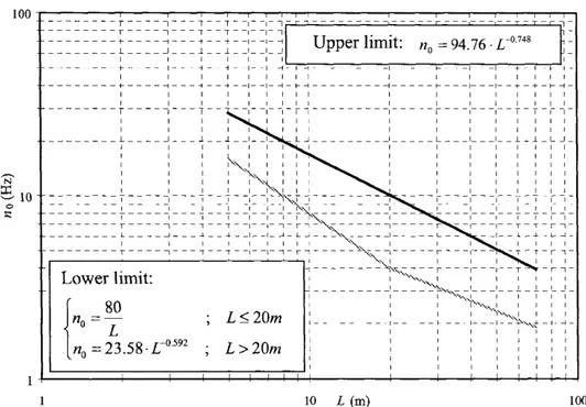
Equation (10) shows that the dimensionless speed corresponding to each resonance situation depends solely on the values of «, / and the Lid ratio. Now the question remains to be fixed whether such values of a are attainable for today's high-speed trains. In this regard, it is known that Eurocode 1 [3] permits the application of a simplified method for evaluating the dynamic effects providing that the span and natural frequency of the bridge belong to the band shown in Figure 2; if such band is assumed as the usual range of pairs {span length, fundamental frequency} in railway bridges, then a realistic maximum value of a for each Lid can be estimated. This is accomplished as follows.
First, realistic minimum and maximum values of span length are computed for each Lid ratio. This is a straightforward calculation considering the maximum and minimum values of d mentioned in the preceding section:
^ = 1 3 . 1 4 - ~L jd.
T
max = 26.4-~L
~d (11)
Equations (11) define an interval [Zmm, LmaX] in the horizontal axis of Figure 2. The
maximum dimensionless speed in that interval is obtained when V is maximum and the product (noL) is minimum (recall that «0 represents the fundamental frequency in
Hz, i.e., the inverse of the fundamental period T). From the mathematical expressions of the upper and lower limit of the band in Figure 2, it can be shown that, within an interval of spans [Lm[n, Lmax], the minimum value of (no L)
corresponds to the point defined by the minimum length Lm{n and the lower limit of
the band. In other words, if L^n <L< L^^ , then the minimum value of {noL) is
(nnL) . = ' 8 0 ^
vAmn J
•Lmn =80 mm
(n0L) ={23.5S-L-^92)-Lc V 0 /mm \ mm / n
Lmm<20m
Lmm >20m mm
(12)
Fmax = 1-2 • 350 = 420 km/h is considered, the steps required for computing the
maximum dimensionless speed for each Lid ratio are the following:
Fix a value of Lid —» Compute Zmm and ZmaX from Equations (11) —>
Compute (^o^)min from Equations (12) —> Determine o w = Vmax I (noL)t
100
x 10
-1 -1 -1 -1 -1 -1—r
i i i i i i i i i i i i i i i i i i i i i i i i -r + 1 I i i i I I I i i I i i _l _ X J I I I I I I - 4 -I I I I -I - 4 -I I I I _ L J . J I I I _l _ X J f----H---f-]--|--|-H
Upper limit: n0 = 94.76 • L~0148 i i
i i
I I I V ^ I I I I i i i ' ^ " " N w i i i i i i l l i ^ ^ ^ ' ' x j x x i r^A i_ j
! i i k j ^ ^
i ' _ '--I j _ X ' . _ _ _
X - I 4 X I I -J L I I I I I I I I r -| T T \~ i -i r
Lower limit:
J no ~ — ', L< 20m [n0= 23.58 -r0592 ; L>20m
1 1 1 1 — i — i — i — i
-;
-x
:
t
— — i — i — _ i —+ _+ _ (_ i i i i i i 1 — i — i —+ - + - 1 -i -i -i -i -i -i i i i i i i i i
H
f
-i -i -i -i -i -i -i
L 1 1 X X L J
1 1 1 1 1 1 1 ^ ^ ^ ^ 1 1 1 1 1 1 1
1 * ^ ^ - | 1 T ~ T ~ 1 1
-1 ^ ^ t -1 l -1 -1 -1
r i ^ ^ ^ T T i — ' Nvv - - *- —'—•- - ^ -r ^
-! X [ i i
i 1 1 — + V v , ; j i i -i -i -i -i -i -i -i
I 1 1 1 — i — i — i 4
-10 L (m) 100
Figure 2: Range of applicability of the simplified method proposed by Eurocode (assumed here as the usual range of spans and frequencies).
Table 1 shows the values of Lid ratio selected for the analysis, along with the corresponding values of L^m and Z,max (obtained from Equations (11)), £ W , Cfe,i
(resonance situations of the second mode) and Amax. A shaded cell in Table 1 indicates that, for that particular value of Lid, ckj > a^^ and therefore the associated resonance of the second mode takes place at speed higher than 420 km/h.
A is a useful parameter that represents the ratio of the distance travelled by the train during one fundamental period (VT) and the characteristic distance between axle loads (d):
A VT L d d
T 2
^ L n
a i
As can be seen, the values of A at resonance (A„,y) depend only on the mode number («) and resonance number (/'). The first four resonances of the second mode correspond to A = 4, 2, 4/3 and 1, respectively. As for the resonances of the first mode, the associated values of A are 1, 1/2, 1/3 and 1/4. Comparing these values with Amax = OmnciLId) is an alternative way of determining which resonance situations can be attained at speed lower than 420 km/h.
Lid 0.3 0.5 0.75 1.0 1.25 1.5 1.75 2.0 2.25 2.5 2.75 3.0 3.25 3.5 3.75 4.0
£min ( m )
3.9 6.6 9.9 13.1 16.4 19.7 23.0 26.3 29.6 32.9 36.1 39.4 42.7 46.0 49.3 52.6
^max ( m )
7.9 13.2 19.8 26.4 33.0 39.6 46.2 52.8 59.4 66.0 72.6 79.2 85.8 92.4 99.0 105.6 flmax 1.46 1.46 1.46 1.46 1.46 1.46 1.38 1.31 1.25 1.19 1.15 1.11 1.07 1.04 1.01 0.99 «2,1 13.33 8,00 5.33 4.00 3.20 2,67 2.29 2.00 1.78 Jt.60 1.45 133 1,23 L14 1.07 LOO «2,2 6.67 4.00 2.67 2.00 1,60 1.33 1.14 1.00 0.89 0.80 0.73 0.67 0.62 0.57 0.53 0.50 Gfe,3 4.44 L 2.67 1,78 1.33 1.07 0.89 0.76 0.67 0.59 0.53 0.48 0.44 0.41 0.38 0.36 0.33 «2,4 3.33 2.00 1.33 1.00 0.80 0.67 0.57 0.50 0.44 0.40 0.36 0.33 0.31 0.29 0.27 0.25 -»Vnax 0.44 0.73 1.10 1.46 1.83 2.19 2.42 2.61 2.80 2.98 3.16 3.32 3.49 3.64 3.79 3.94
Table 1. Minimum and maximum span length as a function of L/d; dimensionless speeds ohj., and maximum values of a and A in the high-speed range (o^x).
In Section 5, A will be used as abscissa in several graphics displaying results of the analysis. Furthermore, for each value of Lid in Table 1, one thousand different values of speed Fhave been selected for the analysis; these values have been equally distributed between 0.9-Fi^ and 1.1 -F^i m order to include the first four resonance
situations of the first and second mode. Accordingly, the values of A in the horizontal axis of the graphics mentioned above will range from 0.9-Ai;4 = 0.225 to
1.1 A.2,i = 4.4. The reason for using such a large number of different speeds was the necessity of computing the maximum response at resonance accurately accuracy; this proved rather involved sometimes due to the presence of sharp resonance peaks, which eventually caused the selection of a very small interval in the speed range.
Finally, in Table 1 it should be also noted that, since the values 0.3 and 4.0 fall out of the initial range specified for Lid (see Equation (8)), the associated span lengths are respectively shorter than 10 meters and longer than 50 meters.
4.4 Selection of several representative sections for evaluation of
the response
If the maximum response of the bridge is to be determined, several values of the abscissa x must be selected in order to ensure that the overall maximum is computed with proper accuracy. To this end, twenty-one different values of x have been selected; these are equally spaced between two extreme sections corresponding to
xlL = lA (at the first quarter of span) and xlL = A (third quarter of span). The
maximum response will surely occur between these two sections because, as it is apparent from Equation (3), the modal contributions of the first and second mode decrease for xlL < XA and xlL > 3A.
As a result, every two consecutive values of x are separated by A(xlL) = 0.025, leading to the aforementioned twenty-one different abscissas; each of them is associated with one of the following values of x/L ratio: 0.25, 0.275, 0.30, 0.325, 0.350,..., 0.75.
4.5 Characteristics of the bridge
The characteristics of the bridge have been selected so as to facilitate the transformation of the results of the analysis to any other similar system by application of the Similarity Formulae (6).
Hence, the length of the bridge has been fixed equal to one meter, its mass per unit length equal to one kilogram per meter, and the bending stiffness EI has been adjusted so as to produce a fundamental frequency m = 1 Hz. Since the axle loads of the train are equal to one Newton, the results presented in Section 5 can be easily transformed providing that linear behaviour of the bridge is assumed (obviously, this transformation will only be exact if the train consists of 15 equally spaced loads, all of them having the same value). Unfortunately, presenting the results for all values of Lid ratio in Table 1 requires a large amount of space that exceeds the limits of this paper, and therefore only the results for the most relevant cases will be shown.
4.6 Distance between consecutive loads (d)
Since the length of the bridge is equal to one meter, as mentioned in Section 4.5, the sixteen different values of Lid ratio listed in Table 1 are obtained by means of an appropriate modification of the distance d between consecutive loads. Thus, sixteen different trains are obtained, each of them associated with one of the following values of d: 1/0.3, 1/0.5, 1/0.75,1/1, 1/1.25,..., 1/4.
5 Results
5.1 Influence of the second flexural mode on the response of the
bridge
Since the investigation presented in this paper is based on a numerical analysis over a range of variation of several parameters, the conclusions that can be extracted, if affirmative, can not be guaranteed to hold for values of such parameters different than the ones considered here. Therefore, the approach of the investigation is opposite to the search of affirmative conclusions; indeed, as will be explained below, we shall try to establish whether a number of statements are not valid in some particular cases.
To this end, the assessment of the bridge response has been carried out for three different quantities: vertical displacement, vertical acceleration and bending moment. As mentioned in previous sections, sixteen values of Lid ratio have been considered, and the maximum values of the three response variables have been computed for twenty-one different locations along the span of the bridge; the analysis has been performed for one thousand different values of the speed, equally spaced between 0.9- V\^ and 1.1 • Vi,\.
Specifically, the purpose of the analysis is to give an answer to three different questions. Considering that the maximum design speed is 420 km/h, and therefore the values of A = VT/d must be less or equal than Amax (see Table 1), the questions to
be answered for each value of Lid ratio are the following:
1) Is the maximum response obtained at mid-span?
2) If answer to question 1) is negative, is the maximum response obtained at the sections corresponding to xlL = lA or xlL = 3A ?
3) Regardless of the answers to questions 1) and 2), are the maximum values of the response computed at xlL = lA or xlL - 3A identical?
As can be seen from Equation (3), the contribution of the second mode to the response at mid-span is zero for displacements, accelerations (second time derivative) and bending moments (proportional to the second spatial derivative). In addition, the contribution of the first mode to the values of such variables is maximum precisely at mid-span, and therefore, if answer to question 1 is affirmative in a particular case, the influence of the second mode in that case can be ignored. Question 1, in conclusion, aims at ascertaining if there are situations where this influence can not be neglected.
As regards question 2, if the maximum response is not obtained at mid-span, this is obviously due to the contribution of the second mode. Since the maximum displacement, acceleration and bending moment associated with this contribution are obtained at xlL = lA and xlL - 3A, it is of interest to establish if the overall maximum
(sum of the effects of first and second mode) is also obtained at those sections. If this were not so, the computation of the response at intermediate locations (such as
x/L = 0.3, 0.4, etc.) would reveal as a crucial part of the analysis.
Finally, with question 3 we try to find out if there are cases when the response at the section located at the first quarter of span is significantly different from the response at three quarters of span.
The answer to all three questions is given within a tolerance of 5%, i.e., if the maximum response is not obtained at span but the response obtained at mid-span is 95% of the maximum or greater, an affirmative answer is given to question 1. Similar treatment is given to questions 2 and 3.
The results of the analysis allow us to extract the following conclusions:
A) At speed lower than 420 km/h (A < AmaX) the maximum displacement and
bending moment is obtained at mid-span for all sixteen values of Lid ratio. Therefore, in all cases the answer to question 1 is affirmative as regards displacements and bending moments and, consequently, question 2 does not require an answer.
B) On the contrary, for five values of Lid, the maximum acceleration is not obtained at mid-span. These values are 1.5, 1.75, 2.25, 2.5 and 3.75. In all these cases the maximum acceleration is computed accurately at both sections xlL =
lA and xlL = %, and therefore question 2 is answered affirmatively. A more
detailed analysis of these five situations reveal the following facts:
B.l) For Lid- 1.5 and 2.5 cancellation of the first resonance of the first mode occurs (see Section 5.2) and the third resonance of the second mode (A = 4/3) becomes prevalent; respectively, the maximum acceleration is approximately 15% and 11% greater than the maximum value obtained at mid-span.
B.2) For Lld= 1.75, 2.25 and 3.75 the second resonance of the second mode (A = 2) is predominant notwithstanding that there is no cancellation of the first resonance of the first mode. In these three cases the maximum acceleration outweighs the maximum value computed at mid-span by 11%, 6% and 6%, respectively. Figure 3 shows the maximum accelerations for Lid = 2.25; in that figure it can be observed that, at speeds lower than 420 km/h (A < Amax = 2.80, indicated by the vertical
dashed line in Figure 3), real cases can be found such that the acceleration at xlL = lA surpasses the one corresponding to xlL = Vi. One
example of this behaviour is that of a bridge of length L - 36m and fundamental frequency «o = 3.5 Hz traversed by a train with
characteristic distance d - 16 m. For these bridge the second resonance of the second mode is attained at V2,i = 2-3.5-16-3.6 = 403.2 km/h.
C) With reference to question 3, the answer is affirmative for displacements and accelerations for all sixteen values of Lid. Conversely, bending moments atx/L = 3/4 are higher than at xlL = VA for Lid = 0.5, 1.0 and 1.25 (8%, 6% and 10%
recall that this conclusions are restricted to speeds such that A < Amax. Figure 4 shows the maximum bending moments corresponding to Lld= 1.25.
•x/L = 1/2
Figure 3: Maximum acceleration atx/X = lA and x/L = % for Lid'= 2.25.
1.4
1.2
d
0 0
-x/L = 1/4
•x/L = 3/4
0.5
Am a x — 1.83 5
1 1.5
A=VT/d
Figure 4: Maximum bending moment at x/L - rA and x/L = % for Lid - 1.25.
Finally, if the limitation V< 420 km/h is ignored and the results of the analysis are examined for the entire range of speeds, i.e., 0.9-Fi,4 < V< 1.1-F^i (0.225 < A < 4.4), the following conclusions can be obtained:
D.l) The maximum displacement is obtained at mid-span for the sixteen different values of Lid.
D.2) Most of the times the maximum acceleration is not obtained at mid-span, but can be computed accurately at x/L = lA or x/L = 3A. The reason is the
large acceleration associated with the first resonance of the second mode, as shown in Figure 5 for Lid - 3.75. Sometimes the value at xlL = XA and xlL = 3A is very similar (the difference is less than 5%), but this is not
always so. Nevertheless, the overall maximum well estimated from one of these two sections for all values of Lid considered in the analysis.
12
10 -- x/L = 1/2
x/L = 3/4
A
s i a. k J<r
<-.vvv.
^ ^ ^ > ^ \ w ^
^ \ I > -
n~> w ^s<fi\ ?* /
0
0 0.5 1 1.5 2 2.5 3 3.5 4 4.5
A=VT/d
Figure 5: Maximum acceleration at x/L = Vi and x/L = 3A for Lid= 3.75.
D.3) ¥ovLld= 0.3, 1.25, 1.5, 2.5 and 3.5 the maximum bending moment is not obtained at mid-span. Besides, for Lld= 0.3 and 3.5 the values computed at x/L - XA and xlL = 3A underestimate the overall maximum by more than
5%.
D.4) The maximum displacements at xlL = lA and x/L - 3A have been found to
5.2 Cancellation of resonance
Yang et al. derived in [13] the mathematical condition of cancellation for the resonances of the first mode. Restricting the discussion to the first four resonances, this condition can be expressed as
4 = H T ^ '' = 1,2,3,4 7=1,2,3,... (14)
a 2i
In Equation (14) all the variables retain their usual meaning, and thus / represents the resonance number; in addition, j is an integer number taking values equal to or greater than unity. If Equation (14) is satisfied exactly the /th resonance of the first mode will not take place even if the velocity of the train is equal to the theoretical resonance speed V\j. If it satisfied approximately, the resonant amplification will be kept to a low level. This interesting relationship explains why high-speed trains can not induce resonance situations in some railway bridges; an example of such behaviour is the passage of an ICE-2 over a 40 meters simply supported bridge: for this train, the characteristic distance between consecutive groups of loads is equal to 26.4 meters, leading to Lid = 40/26.4 = 1.515. This value corresponds approximately to the ratio Lid predicted by Equation (14) for i = 1 andy = 2.
Equation (14) also predicts the cancellation of the first resonance of the first mode when / = 1 and j = 1, i.e., when Lid = 0.5. Several examples analysed by means of numerical simulations and closed-form solutions of Equation (1) seem to contradict this statement, but nevertheless no mathematical proof of this fact has been derived by the authors of this paper, so the question should be treated with due concern.
Similarity Formulae (4.a) and (4.b) guarantee that if cancellation of resonance occurs for a certain train-bridge system, it will also occur for all similar systems. Based on this fact, some interesting conclusions can be drawn from the calculations carried out in Section 5.1. As explained in that section, a train consisting of 15 equally spaced loads has been considered and the closed-form solution of Equation (1) has been obtained for all Lid ratios contained in Table 1. The results of this analysis have furnished the values of Lid such that cancellation occurs. This values are shown in Table 2. It should be emphasised that Table 2 does not contain all possible values of Lid causing cancellation of resonance; instead, it contains only those values causing cancellation among the sixteen different Lid ratios listed in Table 1.
6 Conclusions
The results of the investigation presented in this paper can be summed up in the following general conclusions:
(1) At speeds lower than 420 km/h, for sixteen different values of Lid ratio comprised in the interval 0.3 < Lid < 4.0, no case has been found such that the maximum displacement and bending moment are not obtained at mid-span.
Lid 0.3 0.5 0.75 1 1.25 1.5 1.75 2 2.25 2.5 2.75 3 3.25 3.5 3.75 4
First mode (« = 1)
i = 4 i = 3
X X X X i=2 X X X X X X X
1 = 1
X
X
X
Second mode (n = 2)
i = 4
X X X X X X X X X X X X X X X
1 = 3
X
X
X
X
1 = 2
X X X X X X X
1 = 1
X
X
X
Table 2. Values of Lid among those contained in Table 1 such that cancellation of resonance occurs for the first and/or second mode (values marked with "X").
(2) On the other hand, it has been confirmed that in several cases the maximum acceleration does not correspond to the mid-span section. This is due to the development of resonance situations associated with the second flexural mode, and consequently the contribution of this mode can not be disregarded. In these cases the maximum acceleration can be computed accurately either at the first quarter of span or at three quarters of span since there is very little difference between the results at these two sections. It is of interesting to mention that, since that the maximum value at mid-span is not exceeded by a large amount, it is likely that the maximum accelerations would take place at this section providing that the damping ratio assigned to the second mode was higher than the one assigned to the first mode.
(3) If the speed range is extended in order to encompass the first four resonances of the first and second mode, the maximum displacement is still obtained at mid-span for all sixteen values of Lid. On the contrary, several cases can be identified such that the maximum bending moment is obtained at other sections of the bridge. In addition, only in a few cases the maximum acceleration corresponds to the mid-span section: this is a consequence of the high accelerations produced by the first resonance of the second mode.
References
[I] ERRI D-214 Committee, "Ponts-Rails pour vitesses > 200 km/h et < 350 km/h. Conditions de deformation dynamiques", 1997. ("Railway Bridges for Speed > 200 km/h and < 350 km/h. Conditions of dynamic deformation", Technical Report, 1997, written in French).
[2] ERRI D-214 Committee, "Ponts-Rails pour vitesses > 200 km/h. Rapport Final", 1999. ("Railway Bridges for Speed > 200 km/h. Final Report", Technical Report, 1999, written in French).
[3] European Committee for Standardization (CEN), "Eurocode 1: Actions on structures. Part 2: General actions—Traffic loads on bridges. 2nd Draft",
European Standard, 2001.
[4] L. Fryba, "Dynamics of Railway Bridges", Thomas Telford, 1996.
[5] L. Fryba, "Dynamics of solids and structures under moving loads", 3rd ed.,
Thomas Telford, 1999.
[6] M. Klasztorny, J. Langer, "Dynamic Response of Single-Span Beam Bridges to a Series of Moving Loads", Earthquake Engineering and Structural Dynamics, 19, 1107-1124, 1990.
[7] J. Li, M. Su, "The Resonant Vibration for a Simply Supported Girder Bridge under High-Speed Trains", Journal of Sound and Vibration, 224(5), 897-915, 1999.
[8] P. Museros, "Interaccion Vehiculo-Estructura y Efectos de Resonancia en Puentes Isostaticos de Ferrocarril para Lineas de Alta Velocidad", Tesis Doctoral, Universidad Politecnica de Madrid, 2002. ("Vehicle-Bridge Interaction and Resonance Effects in Simply Supported High-Speed Bridges", Ph. D. Thesis, Technical University of Madrid, 2002, written in Spanish). [9] P. Museros, G. Vivero, E. Alarcon, "Moving Loads on Railway Bridges: the
Spanish Code Approach", Proceedings of the fourth European Conference on Structural Dynamincs (Eurodyn '99), 2, 675-680, A.A. Balkema, 1999.
[10] P. Museros, E. Alarcon, "An Investigation on the Importance of Train-Bridge Interaction at Resonance", Proceedings of the Sixth International Conference on Computational Structures Technology, Civil-Comp, 2002.
[II] P. Museros, M. Romero, A. Poy, E. Alarcon, "Advances in the Analysis of Short Span Railway Bridges for High Speed Lines", Computers & Structures, 80 (27-30), 2121-2132, 2002.
[12] M. Olsson, "On the fundamental moving load problem", Journal of Sound and Vibration, 145(2), 299-307, 1991.
[13] Y.B. Yang, J.D. Yau, L.C. Hsu, "Vibration of simple beams due to trains moving at high speeds", Engineering Structures, 19(11), 936-944, 1997.